Measuring
Tr
non Single Copies of
Using Random Measurements
S. J. van Enk1,2and C. W. J. Beenakker31Department of Physics and Oregon Center for Optics University of Oregon, Eugene, Oregon 97403, USA
2Institute for Quantum Information, California Institute of Technology, Pasadena, California 91125, USA
3
Instituut-Lorentz, Universiteit Leiden, P.O. Box 9506, 2300 RA Leiden, The Netherlands
(Received 5 December 2011; published 16 March 2012)
While it is known that Trn can be measured directly (i.e., without first reconstructing the density matrix) by performing joint measurements onncopies of the same state, it is shown here that random measurements on single copies suffice, too. Averaging over the random measurements directly yields estimates ofTrn, even when it is not known what measurements were actually performed (so that cannot be reconstructed).
DOI:10.1103/PhysRevLett.108.110503 PACS numbers: 03.65.Ta, 03.65.Wj, 03.67.a
The standard textbook quantum measurement of an ob-servableO^ on a given quantum system produces an esti-mate of the expectation value TrðO^Þ, where is the density matrix of the system. This expectation value is linear in . As is well known by now [1–6], nonlinear functions of the density matrix, such as the purityp2 ¼
Tr2 and its cousins p
n¼Trn for n >2, can be
mea-sured directly, too, without first having to reconstruct the whole density matrix. For this direct measurement method to work, one needsnquantum systems that are all in the same state , plus the ability to perform the appropriate joint measurement(s) on those multiple copies.
Here we point out that estimates of the same nonlinear quantities can be obtained fromrandommeasurements on single copies as well. A random measurement can be assumed to be implemented by performing a random uni-tary rotation on the single copy (possibly including an ancilla which starts off in a standard state), followed by a fixed measurement on the single copy (and possibly on the ancilla). By averaging the measurement results over the random unitaries, one can directly infer estimates ofTrn
[withn¼2;. . .; M, withMthe Hilbert space dimension of the system of interest], without having to reconstruct the density matrix. One point of the averaging procedure is that one does not have to know which random unitaries were in fact applied, and, as a consequence, one cannot reconstruct the density matrix in that case. An example of a random measurement is furnished by intensity measurements of speckle patterns resulting from light (be it two photons, or a single photon, or a coherent laser beam) propagating through a disordered medium [7,8], and in that case the purityp2can (and was indeed) inferred directly from those
measurements (see also [9]).
There is an important difference between the known direct method and the current random method in what quantity exactly is estimated. Suppose one’s source does not produce the same state every single time but instead a statejat tryj. In this case, standard quantum measure-ments of a given observable on J instances j¼1;. . .; J
can still be described by a single density matrix, namely, the mean ¼Pjj=J. Since the random method involves only measurements on single copies, it produces, likewise, an estimate ofTrðnÞ. This requires no assumption about
the quantum systems being uncorrelated or unentangled with each other, since j is obtained by tracing out all degrees of freedom except those of systemj.
On the other hand, a direct measurement would yield an estimate of TrðS ^ j;jþ1;...;jþn1Þ instead, where j;jþ1;...;jþn1is the joint density matrix ofnsystemsj; jþ
1;. . .; jþn1andS^is the cyclical shift operator, which acts on the basis states of the n quantum systems as
^
Sjcjijcjþ1i jcjþn1i ¼ jcjþ1ijcjþ2i jcji. It is
only under the assumption that the states of thensystems are identical and independent (i.i.) that the direct measure-ment yieldsTrn. In fact, the direct measurement is emi-nently suited for detecting that the states arenotidentical [10]. Although the assumption of i.i. states is standard, it is only recently that precise conditions have been stated under which the approximate i.i. character can be inferred [11]. The required permutation invariance is easily en-forced when performing measurements on single copies but not when performing joint measurements on multiple copies [12]. Avoiding this difficulty is the main advantage of the random method.
AnNNrandom unitary matrix, distributed according to the Haar measure, can be easily constructed by the method presented in Ref. [13]. One first constructs a matrix whose elements are independent complex Gaussian varia-bles, and one then performs an orthogonalization of the resulting random matrix (where one small pitfall needs to be avoided [13]). We first consider approximate results for random unitaries, because the resulting expressions are quite simple, and subsequently we will give the more involved exact results.
N is large. With this Gaussian approximation, we can compute the following averages (we indicate averages over the distribution of random unitaries byhi): First, we havehVklVmn i ¼kmln=N. Here and in all of the follow-ing, we assume we have picked some basisfjkig, and we write all matrix elements with respect to that basis. The normalization factor 1=N follows immediately from the fact thatU, of whichV is a submatrix, is unitary, so that
PN
l¼1UklU
ml¼km. Higher-order averages follow from
the Isserlis (‘‘Gaussian-moments’’) theorem [15]. In par-ticular, the only nonzero averages arise from products of
2Kfactors of the form
hVk1l1 VkKlKV
m1n1 V
mKnKi ¼
P
all pairsði;jÞ
kimjlinj
NK : (1)
We now apply the preceding approximate results to the following scenario. Consider an ‘‘input’’ density matrixin
of sizeMM. Embed the system in a larger Hilbert space of sizeN, by constructing a newNNdensity matrix by adding zero matrix elements. Then apply a random unitary
Uto the larger matrix. Finally, consider measurements in a fixed M-dimensional (sub)basis fjkig. The probability
ProbðkÞof finding measurement outcomekis given by
ProbðkÞ ¼X
m;n
in
mnVmkVnk : (2)
This expectation value depends on whatVis, of course, but its average is given simply by
hProbðkÞi ¼X
m;n
in
mnhVmkVnk i ¼1=N; (3)
where we used the fact that TrðinÞ ¼Pminmm¼1. Defining PnðkÞ ¼ hProbðkÞni, the following averages are
obtained by using the Isserlis theorem (up to ordern¼4; subsequent orders can be easily obtained, too, but for our purposes this will do):
P2ðkÞ ¼ ½1þp2=N2; (4a) P3ðkÞ ¼ ½1þ3p2þ2p3=N3; (4b) P4ðkÞ ¼ ½1þ3p22þ6p2þ8p3þ6p4=N4; (4c)
where we defined pn¼Tr½ðinÞn. Inverting these
equa-tions gives estimates of pn in terms of the measurable quantities on the left-hand sides. We denote those estimates by an overbar, e.g., p2 ¼N2P
2ðkÞ 1. We refrain from
giving the other inverse relations now, as we will give the exactrelations below in (8).
We can also compute standard deviations in the (mean) estimates. For example, assuming we average the results for one value of k overNrand random unitaries, then the
statistical error in the estimate of the purity is
ffiffiffiffiffiffiffiffiffiffiffiffiffiffiffiffiffiffiffiffi Nrand1
p
ðp2Þ ¼
ffiffiffiffiffiffiffiffiffiffiffiffiffiffiffiffiffiffiffiffiffiffiffiffiffiffiffiffiffiffiffiffiffiffiffiffiffiffiffiffiffiffiffiffiffiffiffiffiffiffiffi
4p2þ2p22þ8p3þ6p4
q
: (5)
This is an increasing function ofp2,p3, andp4, so that the variance is largest for a pure state and smallest for the totally mixed state in¼1=M.
In an actual experiment, one may not know exactly what the values ofNand/orMare (for instance, this is the case in the speckle experiments of Refs. [7,8]). In such a case,N can be directly estimated from P1ðkÞ through N¼
1=P1ðkÞ. So, we would use
~
p2 ¼P2ðkÞ=P1ðkÞ21; (6)
instead (such estimates we indicate by a tilde). Now this estimate p~2 has a smaller variance than p2 has, simply because the errors inP1ðkÞandP2ðkÞare positively
corre-lated. It is, therefore, better to use p~2 as estimate forp2,
even whenN is in principle known. The numerical results given below will confirm this, also for the exact result for
~
p2. For the estimatesp~3andp~4, however, there is not much
difference between the two methods.
WhenNis not very large, Eqs. (1) and hence (4) are not correct. The exact results, which can be extracted from Refs. [16,17], are still given by (4) upon multiplication of
PnðkÞby the correction factorCn, where
Cn¼ ð1þ1=NÞð1þ2=NÞ ½1þ ðn1Þ=N: (7)
Note that these factors depend only onN, not onM, and the results are valid even whenM¼N. This then leads to the inverse formulas:
p2 ¼D2P2ðkÞ 1; (8a)
p3 ¼12½D3P3ðkÞ 13p2; (8b)
p4 ¼16½D4P4ðkÞ 13p226p28p3; (8c)
with Dn¼ ðNþn1Þ!=ðN1Þ!. Taking into account the correction factors (7) leads to different values for the statistical errors in estimates. It is still true that pure states lead to the largest errors; for those we get
ffiffiffiffiffiffiffiffiffiffiffiffiffiffiffiffiffiffiffiffi Nrand1
p
ðp2Þ ¼
ffiffiffiffiffiffiffiffiffiffiffiffiffiffiffiffiffiffiffiffiffiffiffiffiffiffiffiffiffiffiffiffiffiffiffiffiffiffiffiffiffiffiffiffiffiffiffiffiffiffiffiffi
24ð1þ1=NÞ
ð1þ2=NÞð1þ3=NÞ4
s
: (9)
The right-hand side (slowly) increases with increasingN, frompffiffiffiffiffiffiffiffiffiffiffi52=7forN¼4topffiffiffiffiffiffi20forN! 1.
In order to illustrate the method and the meanings ofN and M, we consider the following examples here. (i) Suppose we have a single photon occupying one ofM input modes. We then apply a random linear optics trans-formation that involvesNMancilla modes. The photon now ends up being coherently distributed over N output modes. We then estimate the probability ProbðkÞ with which the photon ends up in one of a fixed set ofMoutput modes k¼1;. . .; M. This is an example akin to that considered in Refs. [7,8].
(ii) Suppose our system of interest consists of 2 qubits, so thatM¼4. Suppose we have an ancilla qubit in a fixed statej0i, and we apply a random unitary operation to the 3
on each of the three qubits separately in the standard basis. We measure the probability ProbðkÞ of the two qubits ending up in one of the M¼4 combinations k¼
00;01;10;11andthe ancilla ending up inj0i(thus mea-suring only anM-dimensional subspace).
(ii0) There is no need for any ancillas if dealing with a fixed and known number of qubits, say,Q. In that case, we simply haveN¼M¼2Q. We consider only case (ii0) in the following numerical results.
We assume that we run an experiment with a fixed random (‘‘unknown’’) unitary of sizeNsufficiently many times that we get a very good estimate ofProbðkÞfor eachk for the given unitary and the given input state (of sizeM). Subsequently, we average over Nrand random unitaries to
obtainPnðkÞ ¼ hProbðkÞni. From those results we estimate
the values ofp2,p3, andp4.
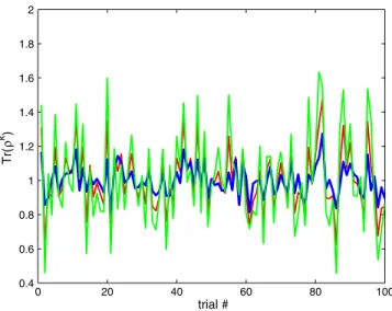
The first example we consider corresponds to case (ii0) mentioned above, where we have two qubits. In Figs.1and
2, we plot results for pure input states, where we use the results for just 1 value ofkto estimatepn, in two different ways: using the exact value N¼4 (Fig. 1) or using the estimateN1=hProbðkÞi(Fig.2). The results show how the latter method is more accurate for estimating purity. The same data are used in the two figures, so that all differences between them are entirely due to the different analysis of those data. This different analysis reduces the statistical variation inp~2 but not inp~3andp~4. In addition,
the plots show that the statistical errors inp~2,p~3, andp~4
are strongly correlated in the latter case.
In the remaining figures, we perform an additional average over theMdifferent values ofk, leading to smaller (by a factor of aboutpffiffiffiffiffiM) error bars.
0 20 40 60 80 100
0.2 0.4 0.6 0.8 1 1.2 1.4 1.6 1.8
trial #
Tr(
ρ
k )
FIG. 1 (color online). This plot shows, for a pure two-qubit state, the estimated values ofp2,p3, andp4(blue,p2; red,p3; green, p4) for 100 trials, each trial using just one value ofk, containing an average over Nrand¼100 random unitaries, and using N¼4 in (8). The mean standard deviations (over 100 trials) were p2¼0:282 [note that this agrees with the result (9), since pffiffiffiffiffiffiffiffiffiffiffiffiffiffiffiffiffiffiffiffiffiffið52=7Þ=990:274], p3¼0:21, p2¼
0:29. The mean estimates obtained by pooling all data from the 100 trials forpn arep2¼0:990,p3¼1:01, andp4¼1:02, which are all consistent with their mean standard deviations (10 times smaller than the pngiven above).
0 20 40 60 80 100
0.4 0.6 0.8 1 1.2 1.4 1.6 1.8 2
trial #
Tr(
ρ
k )
FIG. 2 (color online). The same as the previous figure but using the estimate N1=P1ðkÞ in (8). Here we have ~p2¼
0:09, ~p3¼0:17, and ~p4¼0:27. The mean estimates ob-tained from pooling all data (which are thesame‘‘raw’’ data as in Fig. 1) from the 100 trials forp~n arep~2¼1:005 [which is indeed better thanp2],p~3¼1:01, andp~4¼1:02, all consistent with the statistical errors in the mean (which are 10 times smaller than ~pn).
0 0.2 0.4 0.6 0.8 1
0 0.1 0.2 0.3 0.4 0.5 0.6 0.7 0.8 0.9 1
actual Tr(ρk)
estimated Tr(
ρ
k)
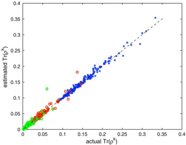
Performing tomography on two qubits would require 15 independent (and known) measurements. Here we show that with just a moderate overhead one can obtain good estimates of p2, p3, and p4 for generic (i.e., randomly picked [18]) states.
In Fig.3, results are displayed for 200 generic two-qubit states, usingNrand¼30.
In Fig.4, we show (for five qubits) that the number of random unitaries needed to obtain a fixed-size error bar does not increase with the number of qubits. For Nrand¼
30, one still obtains good estimates: In fact, the error bars decrease(roughly as1=pffiffiffiffiffiM) when going to more and more qubits, just because the numberMof measurement results one can average over increases exponentially with the number of qubits, while the variance (9) increases only very slowly. This is illustrated for pure multiqubit states in Fig.5. It shows that the statistical error in the estimate of
Trn for n¼2;3;4 first increases with the number of qubits before (at n qubits) it starts to decrease monotonically.
In conclusion then, using the ideas of random matrix theory, we showed that nonlinear functions of the density matrix such asTrncan be directly obtained from appro-priately averaged random measurements on single copies. No assumptions are needed on the independence of the copies nor on their states being identical. This contrasts the random method with so-called direct measurements onn identical copies [1–6].
Moreover, one does not need to know which random measurements were actually performed, because the aver-aging procedure keeps all information about the eigenval-ues of, which is all that is needed to estimateTrn. One does need to verify that the random unitaries have been drawn from the appropriate ensemble. There are two tests
one could perform: First of all, the definition of the en-semble is that it is unitarily invariant. This means in our context that all averageshProbðkÞnishould be independent of k. This is a statistically testable property. In addition, one can apply the random measurements to known input states, so that the values of thosek-independent averages are known.
Importantly, the number of unitaries over which one has to average in order to obtain a fixed error bar in the estimates of Trn scales very favorably with the Hilbert space dimension of one’s system: In fact, this number even tends todecrease. For two qubits this amounts to needing a small overhead as compared to full quantum-state tomog-raphy, but for larger systems (more than, say, four qubits) the random method requires (far) fewer resources than does full quantum-state tomography.
One can implement our method on multiple (say, 4) ions in an ion trap [19,20], for instance, by applying fixed two-qubit gates to randomly picked pairs of ions, inter-spersed with random single-qubit gates, or on the trans-verse spatial degrees of freedom of either single photons or photon pairs, as in Ref. [8].
[1] R. Filip,Phys. Rev. A65, 062320 (2002).
[2] P. Horodecki and A. Ekert, Phys. Rev. Lett.89, 127902 (2002).
[3] P. Horodecki,Phys. Rev. Lett.90, 167901 (2003). [4] H. A. Carteret,arXiv:quant-ph/0309212.
[5] T. A. Brun, Quantum Inf. Comput.4, 401 (2004). [6] F. Mintert and A. Buchleitner,Phys. Rev. Lett.98, 140505
(2007).
[7] C. W. J. Beenakker, J. W. F. Venderbos, and M. P. van Exter,Phys. Rev. Lett.102, 193601 (2009).
0 0.05 0.1 0.15 0.2 0.25 0.3 0.35 0.4 0
0.05 0.1 0.15 0.2 0.25 0.3 0.35 0.4
actual Tr(ρk)
estimated Tr(
ρ
k)
FIG. 4 (color online). The same as Fig. 3 but for randomly pickedfive-qubit states (M¼N¼32). Averaging over the same number of random unitaries (here Nrand¼30) produces a smaller statistical error for larger systems.
2 3 4 5 6 7 8 9 10 11
0 0.05 0.1 0.15 0.2 0.25 0.3 0.35 0.4 0.45
number of qubits
∆
p n
[8] W. H. Peeters, J. J. D. Moerman, and M. P. van Exter,Phys. Rev. Lett.104, 173601 (2010).
[9] A different case is the experiment of M. Munroeet al.,
Phys. Rev. A 52, R924 (1995), where diagonal density matrix elements in the photon-number basis (hard to measure directly) were obtained by phase-averaging more straightforward quadrature measurements.
[10] L. Schwarz and S. J. van Enk, Phys. Rev. Lett. 106, 180501 (2011).
[11] R. Renner,Nature Phys.3, 645 (2007).
[12] S. J. van Enk,Phys. Rev. Lett.102, 190503 (2009). [13] F. Mezzadri, Not. Am. Math. Soc.54, 592 (2007). [14] K. Zyczkowski and H.-J. Sommers,J. Phys. A33, 2045
(2000).
[15] L. Isserlis, Biometrika12, 134 (1918).
[16] B. Collins,Int. Math. Res. Not.2003, 953 (2003). [17] Z. Puchala and J. A. Miszczak,arXiv:1109.4244. [18] As only the eigenvalues of matter, the states
were chosen according to a simple distribution, without significance otherwise: First, M uniformly distributed random numbers (zi) between 0 and 1 are picked; then is chosen as the diagonal matrixdiagðzEiÞ=ðPizEiÞ, with E¼2 in Fig. 3 and E¼8 in Fig. 4. These choices produce a wider spread of values for Trn than do stan-dard ensembles.