A FEATURES ANALYSIS TOOL FOR ASSESSING AND IMPROVING COMPUTATIONAL MODELS IN STRUCTURAL BIOLOGY
Matthew James O’Meara
A dissertation submitted to the faculty at the University of North Carolina at Chapel Hill in partial fulfillment of the requirements for the degree of Doctor of Philosophy in the department of Computer
Science in the Collage of Arts and Sciences.
Chapel Hill 2013
ii © 2013
iii ABSTRACT
Matthew James O’Meara: A Features Analysis Tool For Assessing And Improving Computational Models In Structural Biology
(Under the direction of Jack Snoeyink and Brian Kuhlman)
The protein-folding problem is to predict, from a protein’s amino acid sequence, its folded 3D
conformation. State of the art computational models are complex collaboratively maintained prediction software. Like other complex software, they become brittle without support for testing and refactoring. Features analysis, a language of ‘scientific unit testing’, is the visual and quantitative comparison of distributions of features (local geometric measures) sampled from ensembles of native and predicted conformations. To support features analysis I develop a features analysis tool—a modular database framework for extracting and managing sampled feature instance and an exploratory data analysis framework for rapidly comparing feature distributions. In supporting features analysis, the tool supports the creation, tuning, and assessment of computational models, improving protein prediction and design.
I demonstrate the features analysis tool through 6 case studies with the Rosetta molecular modeling suite. The first three demonstrate the tool usage mechanics through constructing and checking models. The first evaluates bond angle restraint models when used with the Backrub local sampling heuristic. The second identifies and resolves energy function derivative discontinuities that frustrate gradient-based
minimization. The third constructs a model for disulfide bonds.
iv
dependence lead to complex feature distributions. The fourth case study develops a novel functional form for Sp2 acceptor H-bonds. The fifth fits parameters for a refined H-bond model. The sixth combines the
refined model with an electrostatics model and harmonizes them with the rest of the energy function.
Next, to facilitate assessing model improvements, I develop recovery tests that measure predictive accuracy by asking models to recover native conformations that have been partially randomized.
v
ACKNOWLEGEMENTS
I would like to give thanks for the support and guidance I have received in the course of writing this dissertation. Coming from a background in mathematics and being plunged to the worlds of
computational geometry and structural biology I owe a great deal to many people. My primary advisor in computer science, Jack Snoeyink, has shown me the beauty in geometric problems and taught me above all else that careful writing can lead to clear thinking. My primary advisor in biochemistry, Brian Kuhlman, has kindled my excitement for untangling the intricate details of molecular structure and how through studying these details simple and powerful ideas can emerge. I want to thank the institutional support I have received from the UNC Chapel Hill, the Department of Computer Science, NSF, NIH and DARPA for funding my research, and my committee members for their insightful guidance.
Participating in the Rosetta Community thoughout my graduate carrier has allowed me to thrive as a researcher. It was a privilege working shoulder to shoulder with Andrew Leaver-Fay on a range of fruitful projects. I will fondly remember the camaraderie of hacking at the Extreme Rosetta Workshops—thanks to Sam Deluca, Brian Weitzner, Tim Jacobs, Doug Renfrew, Steven Lewis, Will Sheffler, James
vi
vii
TABLE OF CONTENTS
LIST OF FIGURES ... IX
1 INTRODUCTION ... 1
1.1 Overview of Features Analysis ... 2
1.2 Chapter Outline ... 6
1.3 Contributions ... 9
2 BACKGROUND INFORMATION ... 11
2.1 The Structure of Protein Molecules ... 11
2.2 Model Building to Understand Protein Structure ... 14
2.3 Conformational Sampling: From Energy Function to Prediction ... 17
3 THE FEATURES ANALYSIS TOOL ... 23
3.1 Concepts and Terminology ... 23
3.2 The Features Analysis Tool ... 29
4 CASE STUDIES DEMONSTRATING USAGE OF THE FEATURES ANALYSIS TOOL ... 36
4.1 Bond Angle Variation with the Backrub Move ... 36
4.2 Energy Function Smoothness ... 68
4.3 Creation of the dslf_fa13 Disulfide Model ... 80
5 COMPUTATIONAL AND STATISTICAL METHODS ... 84
5.1 Features Database ... 85
viii
6 FEATURE MODELS AND COMPUTATIONAL MODELS ... 100
6.1 Computational Models in Structural Biology ... 100
6.2 Modeling Hydrogen Bonding ... 110
6.3 H-bond Orientation at the Acceptor ... 113
6.4 Parameter fitting ... 136
6.5 Integration of Overlapping Feature Models ... 150
7 STRUCTURE RECOVERY SCIENTIFIC BENCHMARKS ... 164
7.1 Recovery Benchmarks Evaluated ... 166
7.2 Results from Scientific Benchmarks ... 173
8 CONCLUSIONS AND FUTURE DIRECTIONS ... 178
8.1 Summary ... 178
8.2 Scientific Modeling as a Community Endeavor ... 181
8.3 Future Directions and Uses of the Features Analysis Tool ... 183
8.4 Use of Discovered Features in Machine Learning Classifiers ... 184
APPENDIX A: FEATURESREPORTER FRAMEWORK ... 186
APPENDIX B: FEATURESREPORTER CLASSES ... 190
ix
LIST OF FIGURES
Figure 1.1.1 H-bond A-D Distance By Chemical Type ... 3
Figure 2.1.1 Representations of Protein Conformations ... 12
Figure 2.3.1 Decoy Discrimination (Tyka 2010) ... 20
Figure 2.3.2 Deep Decoy Sampling (Tyka 2012) ... 21
Figure 3.1.1 Model Abstraction ... 24
Figure 3.2.1 Components of the Features Analysis Tool ... 29
Figure 3.2.2 HBond feature database schema ... 32
Table 3.2.3 Features Database Schema ... 34
Figure 4.1.1 The Backrub Move (Freidland 2008) ... 38
Figure 4.1.2 N-Cα-C Bond Angle Variation in Natives (Berkholz 2009) ... 39
Figure 4.1.3 Native B-Factors ... 41
Figure 4.1.4 N-Cα-C Bond Angle Native vs. Backrub ... 44
Figure 4.1.5 N-Cα-C Bond Angle by Sample Source and Residue Type ... 50
Figure 4.1.6 N-Cα-C Bond Angle by Residue Type and Sample Source ... 51
Figure 4.1.7 N-Cα-C Bond Angle by Secondary Structure and Sample Source ... 52
Figure 4.1.8 N-Cα-C Bond Angle by in α-helix and Sample Source ... 53
Figure 4.1.9 N-Cα-C Bond Angle by Secondary Structure and Sample Source ... 54
Figure 4.1.10 N-Cα-C Bond Angle by Residue Type, Secondary Structure, and Sample Source ... 54
x
Figure 4.1.12 N-Cα-C Bond Angle by mm_bend Strength and Secondary Structure ... 58
Figure 4.1.13 N-Cα-C Bond Angle by Secondary Structure and mm_bend Strength ... 59
Figure 4.1.14 N-Cα-C Bond Angle by cartbonded Strength ... 61
Figure 4.1.15 N-Cα-C Bond Angle by cartbonded Strength and Secondary Structure ... 62
Figure 4.1.16 N-Cα-C Bond Angle by Secondary Structure and cartbonded Strength ... 63
Figure 4.2.1 Bicubic Smoothing of Backbone Potentials ... 71
Figure 4.2.2 Min Distance From Grid Boundary Q-Q Plot ... 72
Figure 4.2.3 Score12 H-Bond Model Evaluation ... 75
Figure 4.2.4 Score12 H-Bond AHdist Fade Derivative Function Discontinuity Spikes ... 76
Figure 4.2.5 H-Bond AHD CDF by Sample source and AHdist Sliding Windows ... 77
Figure 4.2.6 Score12 H-Bond AHD Pole Accumulation ... 79
Figure 4.3.1 dslf_fa13 Disulfide Model Features by Sample Source ... 82
Figure 4.3.2 dslf_fa13 Model Component Terms ... 83
Figure 5.2.1 Kernel Density Estimation Bandwidth Selection Methods ... 94
Figure 5.2.2 Normalization of the BAH Angle Null Density Distribution ... 95
Table 5.2.3 Maximum Mean Discrepancy to Native: Score12 vs. Talaris2013 ... 99
Figure 6.2.1 H-bonding in Molecular Structure ... 110
Figure 6.3.1 Acceptor Sp2 Functional Groups in Canonical Amino Acids ... 114
Figure 6.3.2 H-Bond BAH, BAχ, and (BAH,BAχ) Feature Definitions ... 117
Figure 6.3.3 Native H-bond Orientation at the Acceptor by Acceptor Hybridization ... 118
Figure 6.3.4 Native H-bond BAH Angle by Acceptor and Donor Type ... 119
Figure 6.3.5 Native H-bond BAχ Angle by Acceptor and Donor Type ... 119
Figure 6.3.6 Native H-bond BAχ Angle by Donor and Acceptor Type ... 120
xi
Figure 6.3.8 Native (BAH, BAχ) Distribution by Sp2 Acceptor Type ... 121
Figure 6.3.9 Baseline H-bond Orientation at the Acceptor by Acceptor Hybridization ... 124
Figure 6.3.10 Baseline H-bond BAH Angle by Acceptor and Donor Type ... 125
Figure 6.3.11 Baseline H-bond BAχ Angle by Acceptor and Donor Type ... 125
Figure 6.3.12 Baseline H-bond BAχ Angle by Donor and Acceptor Type ... 126
Figure 6.3.13 Baseline (BAH, BAχ) Distribution by Sp2 Acceptor Type ... 126
Figure 6.3.14 The Sp2 Model ... 130
Figure 6.3.15 HBondSp2 H-bond Orientation at the Acceptor by Acceptor Hybridization ... 131
Figure 6.3.16 HBondSp2 H-bond BAH Angle by Acceptor and Donor Type ... 132
Figure 6.3.17 HBondSp2 H-bond BAχ Angle by Donor and Acceptor Type ... 133
Figure 6.3.18 HBondSp2 (BAH, BAχ) Distribution by Sp2 Acceptor Type ... 133
Figure 6.3.19 H-Bond Acceptor Orientation in β-sheets ... 135
Figure 6.3.20 Anti-Parallel β-sheet close contact (Hα,O) distance ... 136
Figure 6.4.1 HBondSp2 Model Geometric Features and Chemical Types ... 138
Figure 6.4.2 H-bond AHdist by Sample Source ... 139
Figure 6.4.3 H-bond AHD feature by Sample Source ... 140
Figure 6.4.4 Native H-bond AHdist Feature by Donor Chemical Type ... 141
Figure 6.4.5 Native H-bond ADdist Feature by Donor Chemical Type ... 141
Figure 6.4.6 H-bond AHdist Feature by Acceptor Chemical Type and Sample Source ... 143
Figure 6.4.7 H-bond AHdist Feature by Donor Chemical Type and Sample Source ... 143
Figure 6.4.8 H-bond AHdist Feature by Donor / Acceptor Chemical Type and Sample Source . 144 Figure 6.4.9 H-bond ADdist Feature by Donor / Acceptor Chemical Type and Sample Source . 145 Figure 6.4.10 Native H-bond AHD Feature by Acceptor Chemical Type ... 146
Figure 6.4.11 Native H-bond AHdist Feature by donor Chemical Type ... 146
xii
Figure 6.4.13 H-bond AHD Feature by Donor Chemical Type and Sample Source ... 148
Figure 6.4.14 H-bond AHD Feature by Donor / Acceptor Chemical Type and Sample Source . 149 Figure 6.5.1 Hydryoxyl Donor to Backbone Acceptor H-bonds AHdist Correction ... 153
Figure 6.5.2 Hydryoxyl Donor to Backbone Acceptor H-bonds ADdist Correction ... 154
Figure 6.5.3 Coulombic Model with Atomic Point Charges ... 155
Figure 6.5.4 Rosetta Residue Pair Energies by AHdist ... 158
Figure 6.5.5 Elec + HB: H-Bond AHdist by Sample Source ... 159
Figure 6.5.6 Elec + HB: Carboxyl H-Bonds (BAH,BAχ) by Donor Type and Sample Source 160 Figure 6.5.7 Elec + HB: β-Sheet H-Bonds (BAH,BAχ) by Sample Source ... 161
Figure 6.5.8 Elec + HB: Anti-parallel β-Sheet H-Bonds O-Hα Distance by Sample Source .. 161
Figure 6.5.9 Elec + HB: Serine Acceptor H-Bonds (BAH,BAχ) by Sample Source ... 163
Figure 7.2.1 Rotamer Recovery One Benchmark by H-Bond weight ... 176
Figure 7.2.2 Ab Initio Decoy Discrimination by H-Bond weight ... 177
Figure 8.3.1 Bifurcated Salt Bridge ... 183
1
If we view statistics as a discipline in the service of science, and science as being an attempt to understand (i.e., model) the world around us, then the ability to reveal sensitivity of conclusions from fixed data to various model specifications, all of which are scientifically acceptable, is equivalent to the ability to reveal boundaries of scientific uncertainty.
Rubin, 1984
1 Introduction
The protein folding problem, one of the best puzzles in all of science, is to computationally predict, from a sequence of a protein’s amino acids, the 3D geometry of its stable, biologically active, folded conformation (Anfinsen 1973). State of the art prediction software, such as the Rosetta molecular modeling suite (Rohl et al. 2004, Leaver-Fay 2011), define energy functions over atomic coordinates and stochastically search for low energy conformations. The space of all conformations, whether parameterized in atom coordinates or the angles formed by chemical bonds between atoms, typically has thousands of degrees of freedom. These energy functions are often assumed to decompose into different types of interactions, such as hydrogen bonding, electrostatic attraction and repulsion, rotamer selection, solvent displacement, and salt bridge formation to name a few that will be defined in this dissertation. To make the search manageable, these interactions are often assumed to be local and independent, and a separate model is trained from experimental data for each type of interaction.
2
neighbors), second choosing a functional form, which takes features and tuning parameters and returns an interaction energy (e.g., a function of the distances and angles that are characteristic of hydrogen bonding), and third choosing the values for tuning parameters to fit experimentally observed data distributions. The model is integrated into the software; in Rosetta, this is by adding it as an energy term. The net energy of a configuration is a weighted sum of energy terms, and various benchmarks can be used to tune the weights. The resulting computational models become extremely complex—Rosetta has dozens of energy terms that are active and hundreds that are implemented and available. The model is collaboratively maintained as dozens of researchers tweak and tune, and hundreds use the software for structure prediction and protein design.
A complex computational model, like any other form of complex software, becomes very brittle without good support for testing and refactoring. Modeling decisions made locally can have unexpected consequences, and models developed independently can have unwanted interactions. The thesis of this work is that a features analysis tool for visualizing and assessing distributions of features, which are distributions of geometric measures derived from samples of
conformations, both from native protein structures and from predicted structures with different energy functions, supports the creation, tuning, and maintenance of energy functions, improving protein structure prediction.
1.1 Overview of Features Analysis
3
benchmarks and unit tests. The different plots show distributions of distances from donor to acceptor atoms in a hydrogen bond for different donor types (rows) and acceptor types (columns). For example, backbone/backbone H-bonds are in the last column, second-to-last row. Each plot shows three distribution curves: the red curve is estimated from experimentally determined native structures, the green is from predicted structures that minimize a Rosetta default baseline energy function, and the blue is from predictions that minimize a Rosetta energy with the hydrogen bond energy term replaced by one described in this dissertation. The numbers tell how many pairs each curve is estimated from; the total is nearly 1.5 million bonding pairs.
Figure 1.1.1 H-bond A-D Distance By Chemical Type: Distributions of hydrogen bond acceptor to donor distances, by acceptor and donor chemical types. Each plot shows three distributions: Native (red) is estimated from experimentally determined structures, Baseline (green) and HBondSp2 (blue) ere estimated from predicted structures using different Rosetta energy terms. Numbers indicate how many samples go into each estimation. The blue distributions fit the red more closely than the green for reasons described in the text.
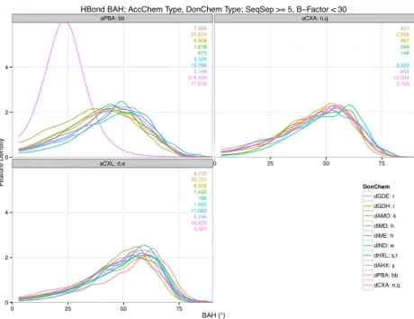
aIMD: h aIME: h aAHX: y aHXL: s,t aCXA: n,q aCXL: d,e aPBA: bb
42 96 89 194 312 215 128 91 63 38 58 60 109 69 59 90 107 84 739 840 823 389 417 329 644 789 793 140 239 223 40 179 139 103 390 237 58 76 37 51 130 141 26 58 55 24 46 40 558 862 1,020 252 295 232 413 691 724 95 263 243 184 600 483 789 1,287 975 293 517 389 185 165 193 89 51 36 242 243 211 619 1,136 1,389 195 298 192 2,271 2,753 2,829 865 1,024 1,025 624 715 582 2,239 1,955 1,446 927 770 627 267 355 348 372 191 170 850 891 785 2,582 3,196 3,148 1,073 1,217 952 8,160 8,247 8,336 3,191 3,791 3,782 633 884 608 2,433 2,480 1,470 848 935 561 171 239 177 226 144 106 2,316 3,186 2,510 819 912 551 9,686 10,103 9,268 2,406 2,648 2,032 7,268 8,473 7,146 17,250 20,211 14,992 5,845 8,696 5,909 1,316 1,382 1,101 1,500 765 511 1,418 1,421 1,285 8,615 10,591 8,566 5,499 5,074 3,649 19,965 21,859 20,400 4,711 5,242 4,084 4,798 6,856 5,358 19,985 19,871 14,241 6,683 6,368 4,116 1,168 1,527 1,220 1,515 948 765 3,432 3,303 3,112 10,951 11,920 11,640 5,153 5,055 4,014 274,457 293,375 292,096 18,374 16,598 14,503 1 3 5 7 1 3 5 7 1 3 5 7 1 3 5 7 1 3 5 7 1 3 5 7 1 3 5 7 1 3 5 7 1 3 5 7 1 3 5 7 dGDE: r dGDH: r dAMO: k dIMD: h dIME: h dIND: w dHXL: s ,t dAHX: y dPBA: b bdCXA: n,q
2.6 2.9 3.2 2.6 2.9 3.2 2.6 2.9 3.2 2.6 2.9 3.2 2.6 2.9 3.2 2.6 2.9 3.2 2.6 2.9 3.2
Acceptor −− Donor Distance (A°)
F
eatureDensity
Sample Source Native Baseline HBondSp2
H−Bond A−D Distance by Chemical Type, SeqSep > 5, B−Factor < 30
4
Backbone/backbone bonds (last column, penultimate row) make up the majority of the data, and the good fits of both the baseline (green) and new HBondSp2 (blue) curves to the natives (red) in these cases actually makes both curves look like good fits in aggregate statistics. In many plots, however, the baseline (green) distribution is too sharply peaked because of an unexpected interaction between the minimizer and internal interpolation between long- and short-range energy terms. Looking down the columns suggest that the green peaks do not depend on donor chemistry type—it was a modeling decision that the functional form of the baseline depends only on acceptor type—but this has unwanted results in rows 7 and 8, where native hydroxyl H-bonds appear to be shorter. HBondSp2 was created and tuned to fit these cases better, and to smooth the interpolation. The shorter hydroxyl H-bonds also necessitated changes to other energy terms in Rosetta, a fact discovered by using the features analysis tool during integration. A model designer who is using the features analysis tool to create the functional form and fit the parameters that better model these types of hydrogen bond can relatively easily create a scientific unit test that can notify him or her if another modeler’s changes to some other energy term moves the distribution of distances outside of acceptable ranges. Then, the two modelers can negotiate a compromise, or even a synthesis, that allows both to achieve their aims.
In my dissertation work, I develop computational tools for assessing and fitting macromolecular energy functions against experimental data. The main tool, which I call features distribution analysis, formalizes an intuitive approach to checking predictive models: comparing ensembles of predictions with ensembles of reference data by looking at distributions of geometric measures, or features. Basing the tool on distributions recognizes that ensembles, rather than single
5
comparing mean lengths tests whether the feature(s) observed in the predicted and experimental conformations are drawn from different distribution.
By choosing biophysically motivated features (e.g., hydrogen bonds lengths and angles, volumes of buried cavities, relative orientation of secondary structure elements, etc.), distributions
obtained from samples can become a language for scientific ‘unit tests.’ These unit tests can be used to give interpretable explanations for preferring one energy function to another. To support these tests, I have created a modular database framework for extracting and managing sampled feature instances and an exploratory data analysis framework for rapidly comparing feature distributions.
I also develop tools to support focused recovery tests that directly measure the accuracy of prediction methods; these help to detect and prevent over-fitting in the more local feature distribution tests. A recovery test asks a model to predict an experimental observation, such as protein conformations observed through X-ray crystallography in a given conformation space. To facilitate rapid energy function evaluation, the conformation can be constrained by, for example, fixing all but a subset of the degrees of freedom. I build upon work within the structural biology community to curate and deploy a collection of new recovery tests. Specifically, I improve the computational benchmarking framework in Rosetta, assembling experimental data and prediction protocols and applying statistically rigorous analysis methods.
To exercise the features analysis tool, as well as to contribute to our understanding of the determinants of molecular structure, I evaluate and refine the H-bond model in Rosetta
6
features analysis tool, I analyze a diversity of H-bond-related feature distributions, evaluating alternative functional forms, and iteratively refining the fit of the model parameters. I use the recovery tests to measure if these modifications improve the overall predictive accuracy. Through this work, I identify and correct specific limitations of the existing model and improve the overall recapitulation of H-bond features observed in experimental data.
To demonstrate that the features analysis and recovery test tools improve molecular structure prediction, I evaluate and integrate several candidate modifications to the Rosetta energy
function. Through scientific benchmarks, I recommend a new standard energy function for the Rosetta community, which has been accepted as the first systematic improvement in nearly a decade.
1.2 Chapter Outline
In Chapter 2, I present structural biology background to establish context for the rest of the dissertation. I first define terminology for molecular conformations (Section 2.1). I then step back to consider the centrality of building and studying models in the scientific process (Section 2.2). Finally, I consider the high computational cost of globally sampling conformations from structural biology energy functions (Section 2.3), which motivates building and studying local feature models.
7
(Section 3.1.2). I support my conceptual foundation by relating it to concepts in computer science, statistics, and structural biology (Section 3.1.3).
In Section 3.2, I describe the tool components and the usage of the features analysis tool by both developers and analysts. Developers implement FeaturesReporters (Section 3.2.3) that populate a features database (Section 3.2.4) and implement features analysis scripts that compare feature instances sampled from the features database through a query (Section 3.2.5). Analysts provide batches of conformation samples, report features to a features database, and run features analysis scripts and interpret the resulting plots and statistics.
In Chapter 4, I present three case studies demonstrating the use of the features analysis tool for checking computational models. I walk through a features analysis step-by-step of the N-Cα-C bond angle distribution when using the Backrub move (Section 4.1). I present three vignettes in which I identify and fix derivative discontinuities in the energy function that frustrate gradient-based minimization (Section 4.2). Finally, I develop a novel model for disulfide interactions that demonstrates the use of features analysis to create components of molecular energy functions (Section 4.3).
In Chapter 5, I elaborate on the computational and statistical methods that underlie the features analysis tool including kernel density estimation, feature transforms, and quantifying divergence of density distributions. I describe desiderata for the tool and how this shapes the design decisions (Section 5.1). I consider mathematical details of density estimation (Section 5.2) and using the features analysis tool to do exploratory data analysis and hypothesis testing.
8
computational models in structural biology (Sections 6.1.1,2). I then Reference Ratio Method, which provides a statistical grounding to the features distribution comparison underlying features analysis (Section 6.1.3-5) and computational methods for weighting feature models (6.1.6). I then discuss prior on work model H-bonds in structural biology (Section 6.2).
Specifically, in the three case studies, I first extend Rosetta’s H-bond model by building an smooth analytic functional form over the (BAH, BAχ) angles to model the orientation dependence H-bonds for Sp2 acceptors (Section 6.3); I second fit the parameters to recapitulate
feature distributions (Section 6.4); and I third harmonize the H-bond model with the rest of the energy function by adjusting the Lennard-Jones model for hydroxyl donors and refitting the H-bond model when combined with a Coulombic potential for electrostatics (Section 6.5).
In Chapter 7, I define recovery scientific benchmarks and use them to evaluate modifications to the Rosetta energy function developed in the case studies. I present 6 recovery benchmarks of increasing difficulty (Chapter 7.1). I then use these benchmarks to evaluate the modifications to the Rosetta energy function presented in Chapters 4 and 6. Based on the positive results, the final energy function combining all the modifications, Talaris2013, has been adopted as the standard Rosetta energy function.
9 1.3 Contributions
My main contribution is the features analysis tool in Rosetta, but I would also like to highlight contributions from my case studies using the tool, and list projects by others in the Rosetta community.
Using the tool for local features analysis has revealed several long-standing anomalies in the Rosetta molecular energy functions, and helped to resolve them, as seen in Chapter 4.
I have advanced the state of the art in modeling of Hydrogen bonding by developing a novel functional form to model H-bonds with Sp2 acceptors, fitting model parameters to recapitulate
native H-bond feature distributions, and integrating an electrostatic model and an explicit H-bond model as detailed in Chapter 6.
I have established community accepted recovery scientific benchmarks and used them along with the feature analyses to demonstrate that my modifications make substantial improvements to the Rosetta energy function. These improvements have culminated in a new standard energy function for the Rosetta Community, Talaris2013 that outperforms Score12, which has been the default for almost a decade.
My improvements to the H-bond model demonstrate local features analysis can guide evaluating and improving complex computational models with substantially less computational cost than globally mapping their behavior as discussed in Section 2.1.
10
Beyond the work I present here, further work that uses one or more components of my features analysis tool include:
• Development of novel feature models
o Development of partially covalent model of hydrogen bonding using atomic orbitals; Steven Combs, Meiler Lab, Vanderbilt University
o Development of a bond length and bond angle feature model and Cartesian space optimization algorithms; Patrick Conway, Baker Lab, University of Washington Seattle
• Use of features database for complex structure prediction and design protocols
o Design of de novo bundle and repeat proteins using a graph of fragments from native structures; Tim Jacobs, Doo Nam Kim; Kuhlman Lab, UNC-Chapel Hill o Development of ligand virtual screening; Sam Deluca, Meiler Lab, Vanderbilt
University
• Descriptive studies of feature patterns
o Analysis of beta turns in anti-body loops; Brian Weitzner, Gray Lab, Johns Hopkins University
o Analysis of cooperative H-bonding and solvation effects Kevin Houlihan; Kuhlman Lab, UNC-Chapel Hill
o Analysis of pH dependent switches in viruses; Joseph Harrison, Kuhlman Lab, UNC Chapel-Hill
• Features database as a means for managing structure prediction data
o Storage of scoring and sequence data for antibody study; Jordan Willis, Vanderbilt University
11 2 Background Information
Before introducing the features analysis tool in the next chapter, we need a few key concepts of modeling protein structure. Because features analysis depends upon conformation space, I review the basics of protein 3D structures and define conformation space (Section 2.1). Features analysis also depends on a view of structural biology as the discipline of building computational models to extend what can determined experimentally and theoretically from a molecular structure (Section 2.2). Features analysis is a direct attack on the computational challenges of working with the complex computational models in structural biology (Section 2.3).
2.1 The Structure of Protein Molecules
12 VRDAYIAKPHNCVYECARNEYCNN LCTKNGAKSGYCQWSGKYGNGCWC IELPDNVPIRVPGKCH
GMRLEKDRFSVNLDVKHFSPEELK VKVLGDVIEVHGKHEERQDEHGFI SREFHRKYRIPADVDPLTITSSLS SDGVLTVNGPRKQVSGPERTIPIT
Figure 2.1.1 Representations of Protein Conformations: Three diagram styles depict conformations of two proteins with codes 1CHZ (top) and 3L1G (bottom). The underlying data for each diagram are the coordinates of the atoms in space, but each representation is a visual model, made using PyMOL (www.pymol.org), that highlights different aspects of the molecular conformation. In a ball-and-stick diagram (left) atoms drawn as colored spheres (red:oxygen, blue:nitrogen, rest:carbon; hydrogens are suppressed), and covalent bonds as lines. A cartoon or ribbon diagram (center) shows the protein backbone, highlighting α-helices and β-sheets. A wire diagram (right) suppresses the spheres to show other information: here Hydrogen bonds are depicted as orange dotted lines.
To give these—and most proteins—their characteristic biological function in nature, the chains of amino acids reliably fold into characteristic 3D structures. Figure 2.1.1 shows the structure for each of these sequences using three different visualizations where the underlying data for each is the coordinates of atoms in space. These conformations were experimentally determined through X-ray crystallography, and the details of the experimental process and the atomic coordinates were deposited into Protein Databank with accession codes 1CHZ1 and 3L1G2.
1 1CHZ is the BmK 2M neurotoxin protein from the Chinese scorpion Buthus martensii Karsch (Li, 1996)
13
To begin to understand the spatial organization of protein structure, consider the degrees of freedom. Chemical bonds that make up the primary structure geometrically constrain the
14 2.2 Model Building to Understand Protein Structure
To understand the natural world, scientists build models: simple systems that correspond to more complex systems of interest. Scientific models are useful because, investigation of the model system can provide information about the more complex system. Through the correspondence, the simpler system is said to represent the more complex system. A simpler representation should not reproduce every detail of the more complex system; the application must dictate which aspects of the more complex system to reproduce and which are not needed.
Consider the visual representations for molecular conformations shown in Figure 2.1.1. The ball-and-stick diagrams in the left column show heavy atoms and bonds and give the viewer some information about the precise location of these atoms in space; however, the overplotting
obscures the spatial relations of some molecules. The right most diagrams highlight the pattern of hydrogen bonding, which contributes to stabilizing the overall fold. Upon close inspection, there appears to be regularity to the H-bonding pattern, though it is still difficult to distinguish. The center diagrams abstract the backbone-backbone H-bonding patterns and show the molecules as ribbon diagrams (Richardson 1981), which highlight the secondary structure: α-helices, β-sheets, and the connecting loops.
15
structure of a naturally occurring protein from its molecular sequence. Because of the relationship between structure and function, increasing our ability to predict protein structure is likely to increase our ability to understand protein function within cells.
In theory, molecular structure is fully described by the laws of Quantum Mechanics. However, solving or even approximating the solutions to the partial differential Schrödinger is
computationally intractable for most biologically relevant proteins because they are such large systems and have delicate energy balances. The gold standard of approximate accuracy for feasible computational QM method scales as O(𝑛!) in the number of atoms (Řezáč 2013).
Since neither experimentally observing protein structure nor directly solving for the structure from first principles is feasible, a primary approach to gaining insight into protein structure is by building computational models to predict protein structure from amino acid sequences. For now, a computational model can be thought of as software used to construct and predict molecular conformations; later I discuss them as realizations of abstract statistical models (Section 6.1).
16
The many successful computational models in structural biology define energy functions over molecular conformation space as linear combinations of feature models, where each feature model evaluates the energy of a type of local geometric observable. With such an energy function, a computational model makes predictions by sampling the conformation space around minima of the energy function. For example, a Markov Chain Monte Carlo sampler (MCMC), defined over a conformation space with a set of local moves, samples observations according to the Boltzmann distribution associated with the energy function as described in the next
subsection.
17
2.3 Conformational Sampling: From Energy Function to Prediction
In this dissertation, I describe my tools to assist the modeling and evaluation of energy functions in structural biology—energy functions that occur in nature probed by experiments, and those defined in computational models. To motivate modeling energy functions by building simple systems to elucidate their behavior, in this section, I discuss why globally mapping the behavior of energy functions is not feasible. The take home messages are that the complexity of the energy functions makes mapping their behavior over conformation space through computational
sampling very demanding and that biased sampling can give misleading results. Additionally, I introduce the FastRelax sampling protocol, which I use in the case studies.
Two canonical sampling methods from statistical mechanics are Molecular Dynamics (MD), which computationally simulates the laws of motion in conformation space, and Markov chain Monte-Carlo (MCMC), which stochastically applies local conformational moves. Either can generate unbiased samples from the Boltzmann distribution3 for an energy function if they satisfy
detailed balance conditions and if the simulations are run long enough. However, because of the complexity of typical energy functions over molecular conformation spaces, it is often
computationally infeasible to generate unbiased samples. Diverse approaches have been
developed to address this challenge, including making full use of computational resources such as GPUs, distributed and parallel computer architectures, and even specialized computer hardware;
3 In statistical mechanics, an isolated system with an energy function 𝐸 𝑐 over conformation space in equilibrium at
temperature 𝑇, adopts the Boltzmann distribution 𝑝 𝑐 =!!𝑒!!!"!, where Z is the normalization constant. Once the temperature has been fixed, the relationship is one-to-one, so the Boltzmann distribution over conformation space is a
lossless model for the energy function. To gain a deeper understanding of the relationship between an energy function,
the Boltzmann distribution and temperature, I recommend investigating simulations of the Ising model, a particularly
18
using coarse grained conformation spaces to reduce the complexity of the problem at the expense of modeling accuracy; and, as I do, using biased sampling strategies but being careful with how the results are interpreted.
A features analysis, which compares distributions of locally defined features that determine global geometry rather than the more global measures such as RMSD to natives, reduces the dimensionality of the problem, increasing the information gained from less costly protocols.
The main sampling strategy that I use to generate decoy sample sources from native chains is the FastRelax protocol in Rosetta (Khatib 2011). FastRelax minimizes the energy function for an input conformation by alternating between a fixed-backbone sidechain optimization (Kuhlman 2000, Leaver-Fay 2008) (repack) and all-atom gradient-based minimization (min) using the (L)BFGS minimizer (Nocedal 2006). The protocol begins with a small weight on Lennard-Jones inter-atom repulsion, to make conformational rearrangement feasible, then alternates repacking and minimizing while ramping up the weight of Lennard-Jones repulsion. FastRelax is written in the relax protocol domain language as
repeat 5
ramp_repack_min 0.02 0.01 1.0 ramp_repack_min 0.250 0.01 0.5 ramp_repack_min 0.550 0.01 0.0 ramp_repack_min 1 0.00001 0.0 accept_to_best
endrepeat
That is, it will accept the best conformation through 5 cycles, each determined by four runs of
ramp_repack_min <fa_rep weight> <min_tolerance> <constraint_weight>
This sets the weight of the repulsive component of the Lennard-Jones model to fa_rep
weight, applies repack, and then applies minimize using min_tolerance as the convergence
19
For the Top8000 set, FastRelax produces conformations with an all-atom RMSD of approximately 1.5 Å from the native, but with distributions of local features that mirror the distributions from more costly protocols, like ab initio. Thus, I am able to use FastRelax for all decoy distributions in the features analyses of this dissertation. For global tests, I use recovery benchmarks, as described in chapter 7.
As an illustration of the challenges of drawing global conclusions from biased samples, let me describe two studies by Tyka and coauthors in which different sampling protocols lead to opposite conclusions. The first, in 2010, found that the energy function of Rosetta was able to find deeper local minima near native structures, and concluded that sampling, rather than energy function quality, was the bottleneck for structure prediction. The second, in 2012, sampled with less bias and found no difference between the depth of local minima for structures that were near or far from native, and concluded that better energy functions were needed.
Here are the details. In 2010, Tyka et al. used Rosetta to generate predictions for a set of 111 proteins of 50 to 150 residues. For each protein, approximately 600,000 predictions were generated using a two-stage protocol known as Iterative Looprelax. The first stage, which aimed to seed the sampling with a diverse range of conformations, used a unified-atom representation of a conformation and performed MCMC optimization with fragment insertions (Simons 1997, Kuhlman 2003). The second stage used FastRelax to find low energy conformations, which are thought to represent stable structures. Depending on the size of the protein, generating a single prediction took approximately 10 CPU minutes. As a result, the whole study required
20
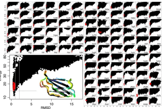
After globally superimposing the lowest energy conformations obtained from the Iterative Looprelax protocol, showed remarkable agreement with the native conformation with 90% of the residues showed less than 0.8 Å deviation from the native structures (Figure 2.3.1) and further many of the discrepancies could be explained by modeled crystal packing artifacts, un-modeled interactions with small molecules, or unstructured loop regions.
Figure 2.3.1 Decoy Discrimination (Tyka 2010): Discrimination of native and non-native conformations (measured by the root mean squared deviation of the Cα atoms (Cα-RMSD) to the native) by the Rosetta energy function. Each cell shows predictions for a native conformation, where each black point is the result of a trajectory of the Iterative Looprelax protocol and each red point is applying FastRelax to the native conformation. The inset target is 1TEN. The vertical gray bars are at 1 Å and 2 Å and the horizontal gray bars are at the lowest energy of the relaxed native conformation. For most targets, the lowest energy conformation has low Cα-RMSD, indicating the energy function is good. However, the bias towards sampling near-native conformations obscures low energy conformations with high RMSD that become visible with more extensive sampling (Figure 2.3.2).
21
1–2 Å Cα Root Mean Squared Deviation (RMSD) of the native structure, as needed for a model to be recognized as native-like based on its very low energy.” This result even suggested that it would be possible to evaluate the quality of a prediction based on this computational benchmark, without always needing to have an experimentally determined structure. An alternative
explanation, however, is that since fragments come from native structures, the seeds were biased toward native or homologous-to-native structures, and thus FastRelax did more extensive search in the neighborhoods of native structures.
Figure 2.3.2 Deep Decoy Sampling (Tyka 2012): Predictions for four targets from the 2010 (dotted line) and 2012 (solid line) study are plotted as the lower envelops of the Cα-RMSD vs. The 2012 study samples more extensively and reveals low energy conformations with high Cα-RMSD indicating the energy function fails to discriminate the native conformation for these targets from non-native conformations.
22
was applied to 31 of the original structures without biasing towards native conformations, many conformations with large RMSD were found to have as low or lower energies than the native conformation. In 14 cases, the folding funnel observed in 2010 was completely erased (Figure 2.3.2). The apparent ability of Rosetta to discriminate native conformations in the 2010 study resulted partially from heavy sampling near native conformations and under-sampling far from native conformations. They conclude, “[f]or the first time in several years, it appears in many cases that successful protein structure prediction is no longer only limited by ability to sample but by accuracy of the energy function.” However, the intense computational cost of sampling prevents use of this protocol for general structure predictions.
23
[S]cientific knowledge advances by practice-theory iteration. Known facts (data) suggest a tentative theory or model, implicit or explicit, which in turn suggests a particular examination and analysis of data and/or the need to acquire further data; analysis may then suggest a modified model and may require further practical illumination and so on.
Box, 1980
3 The Features Analysis Tool
3.1 Concepts and Terminology
This dissertation builds tools to assess computational models of molecular structure against experimental data. To discuss the features analysis tool and its usage rigorously, in this section I define concepts and terminology that characterize the data and how it is analyzed (Section 3.1.1). I then describe a motivating example (Section 3.1.2), which I return to in Section 6.5. I connect the concepts of features and features analysis to unit testing in computer science (Section 3.1.3), Bayesian modeling in statistics (Section 3.1.4), and knowledge-based potentials in structural biology (Section 3.1.5).
3.1.1 Sample Sources and Features
I define a sample source as a process from which it is possible to sample conformations, whether through laboratory experiments or generated from a computational model. By repeatedly
24
For convenience, I use the term native to refer to a sample source whose conformations are experimentally observed, often through X-ray crystallography, then filtered for quality and coverage. These observations produce a model for the behavior of molecular structure in nature, albeit biased by the researchers’ choice of what to experimentally observe, the limitations of the technique, and the filtering process. I use the term decoy to refer to a sample source whose conformations are predicted by software, such as Rosetta, with specified energy functions, optimization methods, and sampling protocols.
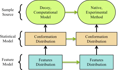
Figure 3.1.1 Model Abstraction: Modeling relationships are depicted as arrows that point from a simpler system to the more complex system it models. The green ovals depict sample sources, which are physical processes that produce molecular conformations either occurring in nature or engineered in computers. The boxes indicate abstract statistical models as probability distributions over either a conformation or a feature space. The green arrows indicate the scientifically relevant modeling relationships. We would like to assess if the decoy computational model accurately represents the native sample source observed through a specific experimental method. Although comparing sample sources or full distributions over conformation spaces are intractable, using features analysis we can compare feature distributions and infer the comparison between sample sources.
I use the term feature throughout this dissertation to mean a measurable quantity of a subset of the atoms in a conformation that may be biophysically relevant. For example, consider the feature AHdist that measures the length of a hydrogen bond (H-bond) (Section 6.1) as the distance between the main acceptor atom and the donated hydrogen atom. A realization of a feature in a conformation is a feature instance (each conformation may have many), and the set of all possible instances forms a feature space.
Decoy, Computational
Model
Native, Experimental
Method
Conformation Distribution Sample
Source
Statistical Model
Feature
Model Distribution Features
Conformation Distribution
25
A sample source induces a probability distribution over a feature space, called a feature distribution, by first sampling a conformation from the sample source and then uniformly sampling a feature from the conformation. For each sample source, each feature is a random variable distributed with respect to the induced feature distribution.
A feature distribution is a model of a conformation distribution, and a conformation distribution is a model of a sample source. Through these correspondences, a feature distribution gives a focused view of a sample source. If a researcher detects a discrepancy between feature
distributions from different sample sources (e.g., natives vs. decoys) by a two-sample test, this implies a discrepancy between the distributions over conformation space and therefore a
discrepancy between the sample sources. This is similar to inferring differences in populations by comparing sample means. I define a features analysis as the use of batches of sampled features to assess and compare sample sources.
3.1.2 Features Analysis as Scientific Unit Testing
From a software engineering perspective, a significant challenge in building complex computational models is assuring the quality of the model. Often biochemical models are
stochastic, so testing for specific numerical results is not meaningful. Instead, researchers express the desired behavior at a much higher level, often in the language of the substantive domain, which may not easily translate into the algorithmic details of the computational model.
26
complex system, often feature distribution test are most naturally expressed as deviations from a reference distribution estimated from the larger system. In this sense, a features analysis becomes a minimal scientific unit test of the computational model.
Software code unit testing, such as through xUnit testing frameworks (Meszaros 2007), allow developers to record that a specific unit of functionality is important to maintain as the code evolves through refactoring and further development (Fewster 1999, Fowler 2002, Beck 2002). To create a code unit test, a developer writes small pieces of test code in a unit-testing framework that exercises the functionality and signals when behavior is broken. Then another developer, or even an end user of the software, runs the unit test through the unit-testing framework to assert that the code is functioning properly.
The process of creating and then running a features analysis scientific benchmark is analogous to creating and running a code unit test. To create a features analysis, a modeler defines a feature through the features reporter framework and creates a features analysis script through the features analysis script framework with the additional requirement that, in addition to plots and summary statistics, the features analysis must return a pass or fail condition. A user or another developer runs the features analysis through the features analysis tool by providing native and decoy samples sources to assert if the decoy feature distribution recapitulates the native feature distribution.
3.1.3 Concepts Related to Features Analysis in the Statistical Modeling Literature
27
the system to be modeled, the prior distribution is updated to the posterior distribution through the Bayes rule. After a model has been fit but before it is used to make inferences or predictions about the larger system, the researcher should check that the model actually fits the data;
Posterior predictive checking does this by computing a summary statistic once from “native” data and multiple times from “decoys” or replicas of the data simulated from the fitted model. The tail probability for the summary statistic of the native data being estimated from the decoy sampling distribution from the model is interpreted as a classical p-value that can be used to reject the model. By choosing summary statistics relevant to the application of the model, posterior predictive checks can detect relevant model violations. Posterior predictive checks can be implemented in the features analysis framework by partitioning the samples from the computational model into replicas.
28 3.1.4 Features Analysis in Structural Biology
Features analysis has long held a prominent role in structural biochemistry, thanks to the availability of highly detailed X-ray crystallography data deposited in the Protein Databank (Berman 2000). In this subsection, I review several landmark studies and recent studies that take advantage of the continued growth in the available experimentally determined structure data. These studies can be classified as describing patterns of molecular geometry for use in tools that validate the quality of experimentally determined or computationally predicted conformations, and for use in tools to generate structure predictions.
Previous studies to identify and classify patterns in native structures suggest several features that can be the basis of features analysis. For example studies of patterns that involve a few residues include those to identify correlations between adjacent bond-lengths and angles (Engh 1991, Berkholz 2009), and torsion angles (Ramachandran 1968, Betancourt 2004). Patterns in sidechain torsion angles have been collected into Rotamer libraries (Ponder 1987, Lovell 2000, Liang 2002), and protein backbones have been classified into regular secondary structure patterns of α -helices and β-sheets, etc. (Richardson 1981, Kabsch 1983, Richardson 1988, Frishman 1995). Studies of non-bonded interactions include characterizing general patterns of charge distribution and H-bonding (Murray-Rust 1984, Baker 1984, Stickle 1992, Kortemme 2003).
29 3.2 The Features Analysis Tool
3.2.1 Overview of the Features Analysis Tool Components
The features analysis tool allows researchers to investigate differences between molecular sample sources by comparing batches of sampled feature instances. The tool builds databases of feature values extracted from given sample sources, whether native or decoy. These can be retrieved, filtered, and compared using graphical data analysis and statistical two-sample tests. Figure 3.2.1 depicts the general workflow.
The features analysis tool is constructed from three components, each of which builds on established technology. The central component is a relational database schema that stores values for sampled feature instances. Storing sampled feature instances in a relational database allows modelers to construct samples of complex features through database queries and rely on robust relational database engines for data management.
Figure 3.2.1 Components of the Features Analysis Tool: Inputs are batches of conformations sampled from sample sources. The upstream component reports elementary features to the features database. The downstream component extracts, transforms, and compares features to assess differences between sample sources.
Features Database Sample
Source
Sample Source
Report Features Report Features
Extract Features Extract Features
Compare Feature Batches Components
Upstream Section 2.2.3
Database Section 2.2.2
30
The upstream component is the features reporter framework and it is responsible for populating the features database from batches of conformations from sample sources. A features reporter module in the features reporter framework is a C++ class that is responsible for populating a set of tables in the database for a conformation. The framework builds on the Rosetta platform, which provides support for representing conformations and making measurements. The features reporter framework is integrated into the RosettaScripts protocol specification language and job distribution system.
The downstream component is the features analysis script framework and it is responsible for creating sampled instances of complex features by querying and transforming data from the features database and analyzing these sampled feature instances. A script in the R statistical programming language is responsible for performing each single analysis and generating graphical and numerical summaries.
3.2.2 Features Analysis Use Cases
31
The features analysis tool is straightforward for analysts to use, even with limited computational experience. An analyst provides a set of conformations representing the sample source, adapts a RosettaScripts protocol to report features and create a features database, adapts a configuration script to run the features analysis scripts, and inspects the results. The ability to relatively easily choose the sample sources and features analysis scripts allows for a variety of comparisons to be performed.
The features analysis tool is flexible for developers to create a wide range of features analyses. Even with limited knowledge of C++ and programming for the Rosetta platform, a developer is able to create simple or complex features reporters that populate the features database. Even with limited knowledge of SQL and R, a developer is able to define a wide range of features and apply a wide range of methods for comparing them. The cost of learning the C++, SQL, and R
languages for developing for the features analysis tool is repaid by the expressive power and the availability of support libraries (e.g., Rosetta in C++ and the wide range of statistical and plotting packages for R).
3.2.3 Features Databases
A relational database consists of a schema that specifies data stored in each table, constraints over single tables or pairs of tables, and a relational database management system (RDMS) that is responsible for storing the data on disk and allowing clients to interact with the database using the Structured Query Language (SQL) or application programming interfaces (Codd 1970).
32
set of conformations sampled from a sample source. Associated with each batch are metadata about the sample source, including software version and command parameters used to report the features, the sampled structures that represent the sampled conformations themselves, and feature data. The feature data is grouped into sets of tables representing closely related features. The set of tables is populated by a features reporter, which is described in Section 3.2.4. Within each set, some tables store sampled values for elementary features while others help define the feature values and the possibly complex relationships to other features. Figure 3.2.2 shows the tables for H-bond related features, and the foreign key relationships between the tables populated by the HBondFeaturesReporter and the batches, structures, and residues tables.
Figure 3.2.2 HBond feature database schema: Each box represents a table and each arrow represents a foreign key constraint. Associated with each H-bond site are the atomic coordinates, and experimental and solvent environment features. Associated with each H-bond are the donor and acceptor sites (stored in the
hbond_sites table), the geometric coordinates (i.e., distances and angles), and the sum of the Lennard– Jones energies for H-bonding atoms.
Recall that a feature is defined as a random variable over a feature space; this means that features are not explicitly stored in the features database. Rather, the values stored in the database are samples from feature random variables. This distinction is important because querying the database can define new features by constraining feature spaces that are their domains. For
hbond_sites+ hbonds+
hbond_site_atoms-
hbond_site_pdb-
hbond_site_environment-
hbond_chem_types-
hbond_geom_coords- residues-
structures-
HBondFeatures--33
example, two different features defined by subsets of the same set of samples are residue types of all residues and residue types of all α-helical residues. The former is stored directly in the
residues table of a features database and the latter can be obtained through a query that joins
the residues table and the residues_secondary_structure table to constrain the DSSP type. Representing feature data as samples in a relational database allows a wide range of features to be accessible with minimal duplication of the actual stored values, making relational databases space efficient.
3.2.4 Reporting Feature to the Database
The upstream component of the features analysis tool facilitates reporting sampled feature values to the features database. C++ classes called FeaturesReporters are responsible for
populating a set of tables. An analyst specifies the features reporters of interest.
I develop on the Rosetta platform a framework that can extract features either from previously generated batches of conformations or on-the-fly from Rosetta-generated predictions.
34
the end of a prediction protocol, features for Rosetta generated predictions can be seamlessly reported to a features database.
From a developer’s perspective, new features can be defined and reported to the database by implementing to a FeaturesReporter C++ interface and building on the functionality available through the Rosetta platform. This process is described in more detail in Section 3.2.5.b.
Batch One Residue Two Residue Multi Residue
Batch Residue Pair Structure
Protocol ResidueConformation AtomAtomPair PoseConformation JobData ProteinResidueConformation AtomInResidue- RadiusOfGyration PoseComments ProteinBackboneTorsionAngle AtomInResiduePair SecondaryStructure
ResidueBurial ProteinBackbone- SecondaryStructureSegment Experimental Data ResidueSecondaryStructure AtomAtomPair Smotif
PdbData GeometricSolvation HBond HelixBundle
UnrecognizedAtom BetaTurnDetection Orbitals StrandBundle
PdbHeaderData Rotamer SaltBridge HydrophobicPatch
DDG Rotamer Recovery LoopAnchor Rigidity
NMR RotamerBoltzmannWeight ChargeCharge VoronoiPacking DensityMap ProteinBondGeometry DFIREPair
MultiSequenceAlignment HelixCapping Energy Function
HomologyAlignment ResidueLazaridisKarplusSolvation Multi Structure ScoreFunction ResidueGeneralizedBornSolvation ProteinRMSD ScoreType Chemical ResiduePoissonBoltzmannSolvation RecoveryBenchmark StructureScores
AtomType Pka ResiduePairRecovery ResidueScores
ResidueType ResidueCentroids ResidueClusterRecovery HBondParameters ResidueTotalScore ResidueGridScoresFeatures
35 3.2.5 Feature Batch Comparison
The downstream framework of the features analysis tool facilitates comparing batches of features stored in a features database. The tool provides a framework for running R-based features
analysis scripts, methods to assist in features analysis tasks, and a community repository for developed features analysis scripts. The prototypical features analysis script specifies input features databases, extracts and filters feature instances, normalizes and transforms them, then compares the batches of feature instances through either summary statistics, visual comparison of distribution functions, or quantitative two-sample tests. I describe details of the functionality supported by the downstream framework in Section 3.2.5.c, below, and demonstrate examples of use in the case studies (Sections 4.1-2 and 6.3-5).
36
4 Case Studies Demonstrating Usage of the Features Analysis Tool
In this chapter, we walk through the first three of six case studies that demonstrate different aspects of the usage of features analysis tool. The first case study (Section 4.1) is a detailed tutorial to show the use of the tool step by step. The second case study (Section 4.2) demonstrates use of the tool to diagnose pathologies in a prediction method. The third case study (Section 4.3) demonstrates the use of features analysis to create a complete feature model and integrate it into an energy function. The remaining three case studies, in Sections 6.3–5, following a discussion of energy based computational models, demonstrate how the tool can be used to create and assess energy functions, tune their parameters, and determine how they should be combined.
Each case study follows the features analysis workflow outlined in Section 3.2—specifying one or more sample sources, storing sampled features into a features database, extracting relevant features and possibly applying transformations, and analyzing feature samples through
exploratory data analysis. Through the analysis, I make observations that suggest further sample sources and feature analyses to explore, which I pursue through iterating the workflow.
Each case study not only demonstrates the features analysis tool, but also addresses a research question in structural biology, showing how the tool helps the researchers to assess and improve their computational models.
4.1 Bond Angle Variation with the Backrub Move
37
question (Section 4.1.1), I define the sample sources and extract features (Sections 4.1.2-3). I specify a features analysis script and use it to compare feature distributions (Sections 4.1.4-6). Additionally, I demonstrate how the features analysis tool can be used to investigate the causes of the observed features by iterating the process (Section 4.1.7-8).
In this case study, I compare N-Cα-C bond angle features from Rosetta decoys generated using the Backrub move against the angles observed in Natives. I confirm the observations from the literature that native N-Cα-C bond angles vary up to 6.5° and depend on the local backbone conformation. I further observe that the recommended sampling bias and bond angle restraint used with the Backrub Move in Rosetta systematically predict N-Cα-C bond angles to be 1.5° too tight (110° vs. 111.5°). Based on this features analysis, I propose an alternative bond angle restraint model that does not have this bias. Further features analysis shows, however, that neither model is able to recapitulate variation by secondary structure classification.
4.1.1 Does the Backrub Move Distort Bond Angles?
The Backrub Move, designed by Ian Davis (2006), is a procedure to locally modify the backbone conformation while keeping the remainder of the structure fixed and he used it as a tool for refining crystal structures by capturing local motion observed in native protein backbones. The Backrub move was adapted in 2008 for the Rosetta platform (Friedland 2008, Smith 2008), since its locality makes it suitable move for Markov chain Monte Carlo conformation sampling