The Hydrangea simulations: galaxy formation in and around massive clusters

The Hydrangea simulations: galaxy formation in and around

massive clusters

Yannick M. Bah´e,

David J. Barnes,

Claudio Dalla Vecchia,

Scott T. Kay,

Simon D. M. White,

Ian G. McCarthy,

Joop Schaye,

Richard G. Bower,

Robert A. Crain,

Tom Theuns,

Adrian Jenkins,

Sean L. McGee,

Matthieu Schaller,

Peter A. Thomas

and James W. Trayford

2_{Jodrell Bank Centre for Astrophysics, School of Physics and Astronomy, The University of Manchester, Manchester M13 9PL, UK} 3_{Instituto de Astrof´ısica de Canarias, C/V´ıa L´actea s/n, E-38205 La Laguna, Tenerife, Spain}

4_{Departamento de Astrof´ısica, Universidad de La Laguna, Av. del Astrof´ısico Francisco S´anchez s/n, E-38206 La Laguna, Tenerife, Spain} 5_{Astrophysics Research Institute, Liverpool John Moores University, 146 Brownlow Hill, Liverpool L3 5RF, UK}

6_{Leiden Observatory, Leiden University, P.O. Box 9513, NL-2300 RA Leiden, the Netherlands}

7_{Institute for Computational Cosmology, Department of Physics, University of Durham, South Road, Durham DH1 3LE, UK} 8_{School of Physics and Astronomy, University of Birmingham, Edgbaston, Birmingham B15 2TT, UK}

9_{Astronomy Centre, University of Sussex, Falmer, Brighton BN1 9QH, UK}

Accepted 2017 June 5. Received 2017 May 31; in original form 2017 March 8

A B S T R A C T

We introduce the Hydrangea simulations, a suite of 24 cosmological hydrodynamic zoom-in simulations of massive galaxy clusters (M200c =1014–1015.4M) with baryon particle masses of∼106_{M. Designed to study the impact of the cluster environment on galaxy formation, they} are a key part of the ‘Cluster–EAGLE’ project. They use a galaxy formation model developed for the EAGLE project, which has been shown to yield both realistic field galaxies and hot gas fractions of galaxy groups consistent with observations. The total stellar mass content of the simulated clusters agrees with observations, but central cluster galaxies are too massive, by up to 0.6 dex. Passive satellite fractions are higher than in the field, and at stellar masses Mstar>1010M, this environmental effect is quantitatively consistent with observations. The predicted satellite stellar mass function matches data from local cluster surveys. Normalized to total mass, there are fewer low-mass (Mstar1010M) galaxies within the virial radius of clusters than in the field, primarily due to star formation quenching. Conversely, the simulations predict an overabundance of massive galaxies in clusters compared to the field that persists to their far outskirts (>5r200c). This is caused by a significantly increased stellar mass fraction of (sub-)haloes in the cluster environment, by up to∼0.3 dex even well beyondr200c. Haloes near clusters are also more concentrated than equally massive field haloes, but these two effects are largely uncorrelated.

Key words: methods: numerical – galaxies: clusters: general – galaxies: stellar content.

1 I N T R O D U C T I O N

In the local Universe, strong correlations exist between the prop-erties of galaxies and their large-scale environment. In particular, galaxies in groups and clusters are typically red, lack recent and ongoing star formation (e.g. Balogh et al.1999; Kauffmann et al.

2004; Weinmann et al.2006; Peng et al.2010; Wetzel, Tinker & Conroy2012), are depleted in atomic hydrogen (HI; Giovanelli &

_{E-mail:[email protected]}

Haynes1985; Fabello et al.2012; Hess & Wilcots2013), and biased towards early-type (elliptical) morphologies (e.g. Dressler1980).

However, all of these properties are also observed to correlate with galaxy luminosity and stellar mass, so that it is possible that these differences stem, at least in part, from different stellar mass distributions between dense environments and the field. The lu-minosity function of cluster galaxies has been studied by several authors in the last decade (e.g. Popesso et al.2006; Agulli et al.

2014,2016; Lan, M´enard & Mo2016). Some of these works indeed found significant variations of the luminosity function between clus-ters and the field, especially in the form of a steep faint-end upturn

C

in clusters (Popesso et al.2006; Lan et al.2016). However, the deep observations of the cluster Abell 85 by Agulli et al. (2014,2016) found no evidence for such a steep upturn. This uncertainty com-plicates the interpretation of the observed environmental variations of galaxy properties.

Stellar mass is arguably a more fundamental quantity than lumi-nosity, but its determination requires estimating the mass-to-light ratio from galaxy colours (e.g. Bell & de Jong2001), or, if available, spectra (e.g. Kauffmann et al.2003a; Gallazzi et al.2005). From an analysis of Sloan Digital Sky Survey (SDSS) spectroscopic data, Kauffmann et al. (2004) demonstrated that a larger fraction of stel-lar mass in dense environments is contributed by more massive galaxies compared to low-density regions. Subsequent studies have suggested that this shift is driven mainly by the special properties of central cluster galaxies (e.g. von der Linden et al.2010): Calvi et al. (2013), for example report that the shape of thesatellitestellar mass function in clusters is similar to that in the field, at least at the massive end. Several other authors, however, have found differ-ences between the satellite and field stellar mass functions, at either the high- or low-mass end (Yang et al.2009; Wang & White2012; Vulcani et al.2014). In part, these differences may be driven by different definitions of ‘environment’ (local density, halo mass, and radial range) and differences in accounting for fore-/background galaxies.

An observational consensus on the nature of stellar mass differ-ences in different environments would clearly be desirable, but even in its absence one can gain valuable insight into the expected extent of, and physical reason underlying, such differences through pre-dictions from theoretical galaxy formation models. Cosmological hydrodynamic simulations are able to self-consistently predict dif-ferences in the formation of central and satellite galaxies, without explicitly prescribing the action of specific processes affecting only the latter. This gives them, in principle, great predictive power to understand the star formation histories of cluster galaxies as mani-fested in their present-day stellar masses.

However, such simulations have for a long time been unable to predict a galaxy stellar mass function (GSMF) in the field that agrees with observations (e.g. Crain et al.2009; Scannapieco et al.2012), which is clearly a pre-requisite for making meaningful predictions about galaxies in clusters. This problem has been solved only re-cently, thanks to increased resolution and, in particular, significant efforts to improve and calibrate the subgrid models that the simu-lations employ to model the unresolved aspects of feedback from star formation and accreting supermassive black holes (BHs). With these improvements, the EAGLE (Schaye et al.2015; Crain et al.

2015) project has produced a simulation that could be calibrated to match the observed stellar mass function and sizes of present-day field galaxies (see also Vogelsberger et al.2014and Dubois et al.2014for the similarly successful Illustris and Horizon-AGN projects). Apart from these calibrated matches, EAGLE has also successfully reproduced, amongst others, the observed colour bi-modality of galaxies (Trayford et al.2015), the evolution of galaxy sizes and star formation rates (SFRs, Furlong et al.2015,2017), their BH mass function (Rosas-Guevara et al.2016) and the correlation between galactic star formation and BH accretion rates (McAlpine et al.2017), their atomic (Rahmati et al.2015; Bah´e et al.2016; Crain et al.2017) and molecular hydrogen content (Lagos et al.

2015), and the environmental effect of galaxy groups on atomic hydrogen (Marasco et al.2016) and galaxy metallicity (Bah´e et al.

2017).

Galaxy clusters, however, occupy only a small volume fraction of the Universe, so that simulation volumes much larger than available

in EAGLE are necessary to sample them in representative numbers. Such simulations can, at present, only afford a much lower reso-lution of5 kpc in spatial terms or particle masses ofmbaryon≈ 109_M

(e.g. Le Brun et al.2014; Bocquet et al.2016; McCarthy et al.2017), compared to 0.7 kpc and∼106_M

for EAGLE. This precludes studying even basic predictions such as stellar masses for galaxies withMstar1010M, while more numerically sensi-tive properties such as their atomic gas content or metallicity are inaccessible for all but the most massive galaxies.

Until simulations at the resolution of EAGLE, but with orders-of-magnitude larger volume, become computationally feasible, progress can still be made through zoom-in simulations, where only a small, carefully selected volume inside a much larger parent sim-ulation is modelled at high resolution and including baryons. The bulk of the volume is instead filled with low-resolution boundary particles interacting only through gravity, whose purpose is the cre-ation of appropriate tidal fields and large-scale modes in the high-resolution region (e.g. Katz & White1993; Tormen, Bouchet & White 1997; Borgani et al. 2002; Dolag et al. 2009; Ragone-Figueroa et al. 2013; Martizzi et al. 2014; Barnes et al.2017a; Hahn et al.2017).

Motivated by these considerations, this paper introduces the Hy-drangeasimulation project,1_{a suite of 24 high-resolution zoom-in} galaxy clusters run with the EAGLE code for the purpose of study-ing the interaction between clusters and the galaxies in and around them. Each high-resolution simulation region is centred on a mas-sive cluster (M200c=1014.0−1015.4M),2and realized at the same resolution level as the largest-volume simulation of the EAGLE project (mbaryon=1.81×106M, gravitational softening length

=0.7 physical kpc atz<2.8). The high-resolution zoom-in region is set up to include not only the cluster haloes themselves, but also their large-scale surroundings out to 10 virial radii, i.e.∼10–25 co-moving Mpc, motivated by indications from observations (e.g. von der Linden et al.2010; Lu et al.2012; Wetzel et al.2012) and theory (Bah´e et al.2013) that the environmental influence on at least some galaxy properties extends significantly beyond the virial radius.

In this paper, we present a validation of the simulations in terms of some of the most fundamental galaxy properties, namely their stellar mass function and quenched fractions atz ≈ 0, and then use the detailed information provided by the simulations to gain insight into the impact of the cluster environment on the GSMF. In a companion paper (Barnes et al.2017b), we analyse the prop-erties of the hot intracluster medium (ICM) in a sample of simu-lated clusters including the Hydrangea suite, and demonstrate that the simulations predict X-ray and Sunyaev-Zel’dovich (SZ) prop-erties that are broadly compatible with low-redshift observational constraints. Predictions for the galaxy luminosity functions in our simulations, including results from a higher resolution run of an intermediate-mass cluster, will be presented by Dalla Vecchia et al. (in preparation). Together, these simulations form the ‘C-EAGLE’ project family.3

This paper is structured as follows. In Section 2, we review the EAGLE galaxy formation model that was used in our simulations, and describe the selection and simulation of the clusters that form

1_{Named after the plantHydrangea macrophylla, whose petals change their} colour from blue to red according to their environment, in analogy to the colour–density relation of galaxies.

2_M

200cdenotes the total mass within a sphere of radiusr200c, centred on the potential minimum of the cluster, within which the average density equals 200 times the critical density.

3_{‘Cluster-EAGLE’, also referring to Steller’s sea eagle (Haliaeetus}

the Hydrangea suite. We then compare several key predictions of the simulations toz≈0 observations in Section 3, followed by a detailed analysis of the simulated stellar mass function in Section 4. Our results are then summarized and discussed in Section 5.

Throughout the paper, we adopt the same flatcold dark mat-ter (CDM) cosmology as used in the EAGLE simulations, with parameters as determined by Planck Collaboration XVI (2014b): Hubble parameterh≡H0/(100 km s−1Mpc−1)=0.6777, dark en-ergy density parameter=0.693 (dark energy equation of state parameterw= −1), matter density parameterM = 0.307, and baryon density parameter b = 0.04825. For length-scales, the prefix ‘p’ and ‘c’ denotes physical and comoving quantities, re-spectively (e.g. ‘pkpc’ for ‘physical kpc’); where no prefix is given, distances are given in physical units. Unless otherwise specified, all galaxy stellar masses are computed as the sum of gravitationally bound star particles within 30 pkpc from the potential minimum of their subhalo (see Schaye et al.2015).

2 D E S C R I P T I O N O F T H E S I M U L AT I O N S

In this section, we first provide a summary of the key features of the EAGLE code that was used for this work (Section 2.1), and then describe the setup and running of the Hydrangea cluster simulations (Section 2.2).

2.1 The EAGLE galaxy formation model

The simulation code developed for the EAGLE project is a substan-tially modified version of theGADGET-3 smoothed particle hydrody-namics (SPH) code, last described in Springel (2005). We restrict our description here to a summary of only its key features and refer the interested reader to the detailed description by Schaye et al. (2015).

Compared to GADGET-3, the hydrodynamics and time-stepping scheme has undergone several updates that are collectively referred to as ‘Anarchy’ (Dalla Vecchia, in preparation; see also appendix A of Schaye et al.2015; Schaller et al.2015c). These include using the conservative pressure-entropy formulation of SPH (Hopkins2013), an artificial viscosity switch (Cullen & Dehnen2010), an artificial conduction switch similar to that of Price (2008), theC2_Wendland (1995) kernel, and the time-step limiter proposed by Durier & Dalla Vecchia (2012). These updates mitigate many of the shortcomings of ‘traditional’ SPH codes, such as the treatment of surface discon-tinuities, described by e.g. Agertz et al. (2007) and Mitchell et al. (2009). Schaller et al. (2015c) discuss the impact of these modifi-cations on the simulated galaxies in detail, and show that the most significant change is due to the Durier & Dalla Vecchia (2012) time-step limiter. These authors also demonstrated that the improved hy-drodynamics implementation is a key requirement for the efficient action of feedback from supermassive BHs, as described further below.

Most importantly, the code contains subgrid physics models that were evolved from those developed for the OWLS (Schaye et al.

2010) simulation project.

Radiative cooling and photoheating rates are computed on an element-by-element basis following Wiersma, Schaye & Smith (2009a), by considering the 11 most important atomic coolants (H, He, C, N, O, Ne, Mg, Si, S, Ca, and Fe) in ionization equilibrium and in the presence of a Haardt & Madau (2001) ionizing UV/X-ray background. As discussed by Schaye et al. (2015), the code does not account for self-shielding of gas, because in the regime where this is expected to be important (nH10−2cm−3), the uncertain

effect of local stellar radiation would also need to be considered (Rahmati et al.2013).

The modelling of reionization follows Wiersma et al. (2009b). To account for hydrogen reionization, the Haardt & Madau (2001) background is switched on at redshiftz=11.5 (Theuns et al.2002a; Planck Collaboration I2014a). This is accompanied by the injection of 2 eV of energy per proton mass. He reionization is modelled by injecting the same amount of energy aroundz=3.5, which results in a thermal evolution of the intergalactic medium (IGM) in agreement with the observations of Schaye et al. (2000, see also Theuns et al.

2002b).

The SFR of gas particles is modelled as a pressure law following Schaye & Dalla Vecchia (2008),

˙

mstar=mgA

1 Mpc−2−nγ

GP

(n−1)/2

, (1)

where ˙mstaris the SFR of a gas particle with massmgand (total) pres-sureP,γ=5/3 is the ratio of specific heats, andGthe gravitational constant. The subgrid parametersA=1.515×10−4_M

yr−1_kpc−2 andn=1.4 are then directly prescribed by observations (Kenni-cutt1998), independent of any imposed equation of state. Deviating from Schaye & Dalla Vecchia (2008), the star formation threshold

n∗

Hdepends on metallicity, as proposed by Schaye (2004):

n∗

H(Z)=10− 1

cm−3

_Z

0.002 −0.64

, (2)

whereZis the gas-phase metallicity smoothed over the SPH kernel (see Wiersma et al.2009b). This equation accounts for the metallic-ity dependence of the transition from the warm atomic to the cold molecular interstellar gas phase.n∗H(Z) is limited to a maximum of 10 cm−3_{to prevent divergence at lowZ. Star formation is then} implemented stochastically with the probability of a gas particle be-ing converted to a star set by equation (1). Because the simulations lack the resolution and physics to directly model the cold dense gas phase in which star formation is observed to occur in the real Universe, a pressure floor corresponding toPeos∝ρ_g4/3is imposed on gas withnH≥10−1cm−3, normalized toTeos=8×103K at that density. As this relation corresponds to a constant Jeans mass, it pre-vents artificial fragmentation due to a lack of numerical resolution (Schaye & Dalla Vecchia2008).

Mass and metal enrichment of gas due to stellar mass loss is mod-elled as described by Wiersma et al. (2009b) with the modifications described in Schaye et al. (2015). This approach is based on treating star particles as simple stellar populations with a Chabrier (2003) initial mass function in the mass range 0.1–100 Mand accounting for winds from asymptotic giant branch and massive stars as well as type-Ia and core-collapse supernovae.

Energy feedback from star formation is implemented in a single thermal mode, by heating a small number of gas particles (∼1) by a large temperature increment (T= 107.5_{K). Dalla Vecchia &} Schaye (2012) demonstrate that this approach alleviates numerical overcooling without the need to temporarily disable hydrodynamic forces or radiative cooling for affected gas particles, but can still not avoid it completely in the regions where the gas density is highest, and the cooling time therefore shortest. As discussed in detail by Crain et al. (2015), the efficiency of star formation feedback is there-fore scaled with gas density so that energy input in dense regions formally exceeds the physically available energy budget from core-collapse supernovae. Averaged over the entire simulation, however, the ratio is below unity. In addition, the efficiency is lowered in high-metallicity gas to account for the physically expected higher cooling losses. Crain et al. (2015) show that these scalings of star formation

feedback efficiency are crucial for obtaining galaxies with realistic sizes, although the total galaxy masses are largely insensitive to them.

We note that, as an undesired side effect, these high-energy, stochastic, local heating events produce gas discs in some simulated galaxies that contain artificially large holes (Bah´e et al.2016). As we discuss further in Section 3.2, these holes may affect the predicted interaction between the dense cold gas discs and the hot intracluster gas in our simulations.

Finally, the code includes a model for the growth of supermas-sive BHs, which are seeded in a friends-of-friends (FoF) halo once its mass exceeds 1010_h−1_M

(Springel, Di Matteo & Hernquist

2005a) with a (subgrid) BH seed mass of 105_h−1_M

. Subse-quently, the subgrid BH mass grows as a consequence of gas ac-cretion, which is modelled as in Rosas-Guevara et al. (2015) but without the Booth & Schaye (2009) ‘boost factor’ (Schaye et al.

2015). In essence, this approach considers the angular momentum of gas near the BH to limit the Bondi accretion rate to

˙

maccr=m˙Bondi×min

C−1 visc

cs/Vφ3,1

(3)

wherecsis the sound speed andVφthe rotation speed of gas around the BH. The parameterCviscwas thought to set the stellar mass at which accretion becomes efficient (Rosas-Guevara et al.2015). However, Bower et al. (2017) have shown that this scale is instead determined by the critical halo mass above which the hot hydro-static atmosphere traps outflows driven by star formation and is nearly independent ofCvisc. In the EAGLE reference model (‘Ref’),

Cvisc=2π.

In analogy to star formation, energy feedback from supermassive BHs (‘AGN feedback’) is implemented stochastically, with one par-ticle heated by a large temperature increment. Following Booth & Schaye (2009), 15 per cent of the accreted rest mass is converted to energy, with a 10 per cent coupling efficiency to the surrounding gas, i.e. an energy injection rate of 0.015 ˙maccrc2(where cis the speed of light). Because the gas surrounding supermassive BHs is typically denser than around newly formed stars, the temperature incrementTAGNmust also be higher to make the feedback effi-cient. In the Ref model, one particle per heating event is heated byTAGN=108.5K. However, Schaye et al. (2015) have shown that this predicts X-ray luminosities and hot gas fractions in galaxy groups and intermediate-mass clusters that are higher than observed. An alternative model that differs from Ref only in its choice of

TAGN(=109K) andCvisc(=2π×102), ‘AGNdT9’, was shown to largely resolve these discrepancies on the scale of galaxy groups, while achieving a similarly good match as Ref to observed proper-ties on galactic scales.4_{As discussed by Schaye et al. (2015), the} increased heating temperature makes individual heating events more energetic and hence reduces numerical cooling losses. The increased value ofCviscwas motivated by a better fit of the GSMF to obser-vations. We therefore adopt the AGN feedback parametrization of AGNdT9 for all C-EAGLE simulations, including the Hydrangea suite presented here. In a companion paper (Barnes et al.2017b), we show that this model also leads to simulatedclusterswith overall realistic ICM properties, albeit with a still somewhat too high hot gas mass fraction (by∼2σ), and artificially high entropy levels in the cluster cores.

4_{Because AGNdT9 was only realized in a (50 cMpc)}3_{simulation volume,} it contains only one halo whose mass atz=0 is (just) above 1014_M

. Schaye et al. (2015) could therefore not test its predictions on the hot gas properties in massive clusters.

2.2 The Hydrangea simulations

2.2.1 Selection of the C-EAGLE cluster sample

The reason for the absence of massive galaxy clusters in the original EAGLE simulations is their relatively small volume of ≤(100 cMpc)3_{. Our new simulations are therefore based on a much} larger ‘parent simulation’, described by Barnes et al. (2017a). This is a (3200 cMpc)3_{volume which was simulated with dark matter} only (DMO), in the same cosmology as that adopted for the EAGLE project (Planck Collaboration XVI2014b, see Introduction). The DM particle mass in the parent simulation is 8.01×1010_M

with a gravitational softening length of 59 ckpc; a galaxy cluster with M>1014_M

is therefore resolved by at least 1000 particles. From the parent simulation snapshot atz=0, we then selected candidate clusters for zoom-in re-simulation. Apart from a threshold in halo mass (M200c≥1014M), we also applied a mild isolation criterion, by requiring that no more massive halo be located within 30 pMpc, or 20r200c, whichever is larger, from any re-simulation candidate (r200chere refers to the radius of the neighbouring, more massive halo). This criterion ensures that our simulations are centred on the peak of the local density structure and not, for example, on a moderately massive halo on the outskirts of an even more massive cluster. Finally, for computational convenience we required that our candidate clusters be no closer than 200 pMpc to any of the periodic simulation box edges.

From this initial list of 91 824 candidate haloes, we then selected a subset of 30 objects for re-simulation. To avoid a bias towards the more common lower-mass haloes, our candidates were binned byM200cinto 10 logarithmic bins from 1014Mto 2×1015M (log10M200c=0.13). Three objects were then selected from each bin at random. To extend our mass range yet further, we only picked two objects from the highest mass bin, and selected a final halo at even higher mass,M200c=1015.34M. These 30 objects comprise the C-EAGLE cluster sample.

2.2.2 Motivation for large zoom-in regions

The virial radius, approximated byr200c, has traditionally been as-sumed to represent the boundary between a halo and the surrounding Universe, based on the spherical collapse model. However, evidence has emerged in recent years that galaxies might be affected by their environment out to significantly larger distances (e.g. Balogh et al.

1999; Haines et al.2009; Hansen et al.2009; von der Linden et al.

2010; Lu et al.2012; Rasmussen et al.2012; Wetzel et al.2012), a result that has been supported by previous generation hydrodynam-ical simulations (Bah´e et al.2013; Bah´e & McCarthy2015). While most observational evidence for this large-scale influence is based on galaxy colours and SFRs, Bah´e et al. (2013) have shown that the GIMIC simulations predict an effect that reaches even further when the hot gas haloes of galaxies are considered instead: in galaxies withMstar ≈109M, these are predicted to be depleted even at

r>5r200cfrom the centre of a group or cluster.

constitute the Hydrangea simulations as analysed in this paper. The remaining six objects, with masses between 1014.6_{and 10}15.2_M

, were simulated only out to 5r200c, primarily serving as tools to study the ICM for which each simulation only contributes one (central) object of interest, as opposed to several hundreds or even thousands of galaxies. The additional C-EAGLE simulations are described in more detail by Barnes et al. (2017b).

2.2.3 Simulation runs and post-processing

The Hydrangea simulations were run mostly on the HazelHen Cray-XC40 system hosted by the German Federal Maximum Perfor-mance Computing Centre (HLRS) at the University of Stuttgart. This system provides nodes with 128 GB of memory each, shared by 24 compute cores for an effectively available 5 GB of memory per core. On this system, we could accommodate most of our hy-drodynamic runs on≤2048 cores to minimize scaling losses in our highly clustered simulations. From initial conditions (ICs) gener-ated as described in Appendix B (see also Barnes et al.2017b), the most massive cluster in our sample required more than 10 million core hours to reachz=0, corresponding to a total wall clock time of over 10 months (including queueing and downtime). Several clusters from the low-mass end of our sample were run on ma-chines at the Max Planck Computing and Data Facility (MPCDF) in Garching.

In addition to these hydrodynamic simulations, we also per-formed one DMO simulation of each zoom-in region. These use the same ICs as the hydrodynamical runs, but due to their non-dissipative nature, they produce less small-scale clustering and hence only consumed<105_{CPU-hr each.}

As main output from the simulations, 30 full ‘snapshots’ were stored betweenz=14.0 and 0. Out of these, 28 are spaced equidis-tant in time (t= 500 Myr), while two additional snapshots (at z=0.101 and 0.366) were included to facilitate comparison to the EAGLE simulations.5_{All snapshots were post-processed with the} SUBFINDcode (Springel et al.2001; Dolag et al.2009) to identify FoF haloes, using a linking length ofb=0.2 times the mean inter-particle separation, and self-bound subhaloes within them. We note in this context that ‘subhalo’ can refer to either the central object that contains the largest fraction of the FoF mass or (where they exist) less massive ‘satellites’.

Subhaloes in the DMO and hydrodynamic runs were individually matched by comparing their unique DM particle IDs, as described by Velliscig et al. (2014) and Schaller et al. (2015a). The 50 most-bound DM particles in each subhalo from the DMO simulation are located in the corresponding hydrodynamic simulation. If one subhalo contains at least half of the particles with the same ID in the hydrodynamic simulation, a link is initiated between the two. This link is then confirmed if, and only if, the original subhalo in the DMO simulation also contains at least 25 of the 50 most-bound DM particles of the corresponding subhalo in the hydrodynamic simula-tion. 92 per cent of central subhaloes withM200c>1011Mcould be successfully matched between the hydrodynamic and DMO sim-ulations in this way.

To reconstruct the evolutionary and orbital histories of individ-ual simulated galaxies, we have linked subhaloes between different snapshots using an updated version of the algorithm described in

5_{Including these two extra snapshots, 12 EAGLE snapshots have a} coun-terpart in Hydrangea with a time offset of50 Myr, including eight at

z2.0.

Bah´e & McCarthy (2015). This method is described in full in Ap-pendix C. In essence, subhaloes in adjacent snapshots are linked by matching their constituent DM particles, taking into account the formation of new galaxies, mergers between them, and temporary non-identification of galaxies by theSUBFIND algorithm in dense environments (see e.g. Muldrew, Pearce & Power2011). We note that this algorithm is similar, but not identical, to that used by Qu et al. (2017) to build merger trees from the EAGLE simulations. Unlike in Bah´e & McCarthy (2015), we base the tracing on DM particles only. This simplification is possible because of the higher resolution of the Hydrangea simulations, which allows DM haloes to be resolved even for galaxies undergoing severe stripping.

In addition, we stored a larger number of ‘snipshots’ that contain only the most important, and most rapidly time-varying, quantities, such as particle positions and velocities (similar to EAGLE; see Schaye et al.2015). We stored three snipshots between each of the 28 main snapshots, for a combined time resolution oft=125 Myr. This was then additionally boosted tot= 25 Myr for three 1-Gyr intervals at lookback times of 0–1, 4–5, and 7–8 1-Gyr. For one intermediate-mass cluster, snipshots were stored at a constant time interval oft=12.5 Myr. In future papers, we will exploit the high time resolution provided by these snipshot outputs to trace the evolution of our simulated cluster galaxies in detail; here, we restrict ourselves to an analysis of the snapshot data, in particular those atz=0 and 0.101.

2.2.4 Visualizations of the simulated clusters

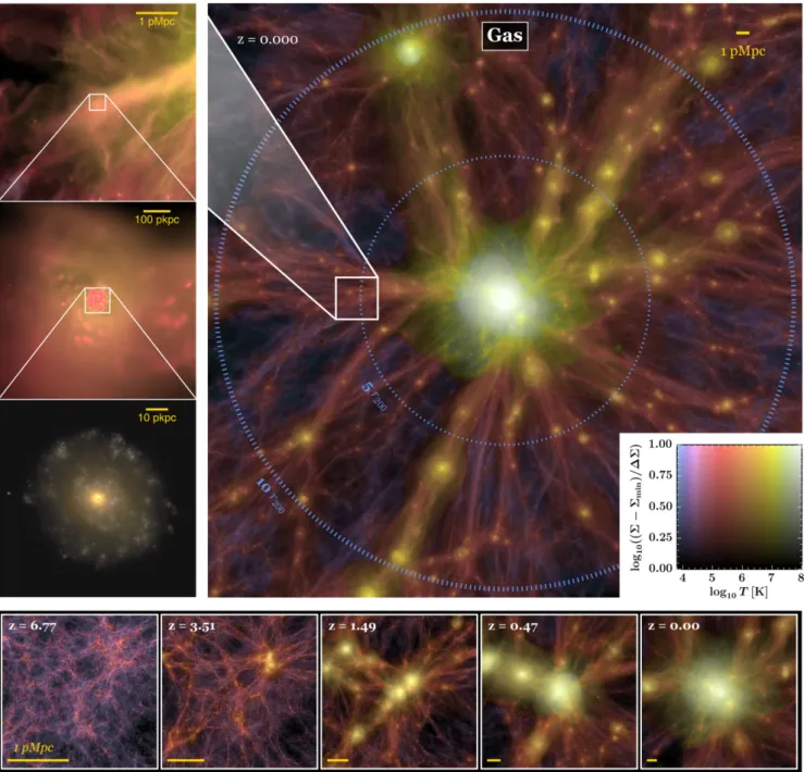
A visualization of one Hydrangea simulation is presented in Fig.1; this contains at its centre the most massive cluster, CE-29, with

M200c=1015.38M.6The main panel shows the gas distribution atz=0 in a slice of side length 60×60 pMpc and thickness 15 pMpc, centred on the potential minimum of the cluster. The colour map, shown in the bottom right inset, encodes both the projected gas density (as brightness) and temperature (as hue/saturation); the coldest gas (T 104_{K) is shown in blue, and the hottest (T} 108_{K) in white. Clearly visible is the central hot (T10}7_{K) halo} that extends to∼4r200c, and a myriad of filaments and embedded haloes out to the nominal edge of our high-resolution region at 10r200c(thick dotted blue line).

The three panels on the left-hand side present successive zoom-ins towards one individual galaxy on the cluster outskirts, highlight-ing the vast dynamic range of the simulation. The top two show the gas density and temperature, using the same temperature scaling as the main panel but with adjusted scaling of the surface density for improved clarity. In the bottom panel, we display a synthetic grioptical image created with the radiative transfer code ‘SKIRT’ (Camps et al.2016; Trayford et al.2017).

The five panels in the bottom row illustrate the formation history of the cluster. Each shows a projected cube of side length 20h−1 cMpc, centred on the main progenitor of thez= 0 cluster. The corresponding physical scale is indicated by the yellow bar in the bottom left corner of each panel, which indicates a length of 1 pMpc. Starting from a web-like structure atz≈7, the simulation forms a number of protocluster cores byz=1.5 which then successively merge to form the present-day cluster. As an aside, we note that

6_{Note that there are small differences between the halo masses in the} low-resolution parent simulation and high-low-resolution hydrodynamic zoom-in re-simulations, by<0.05 dex. As a convention, we denote individual zoom-in regions, and their central clusters, by the prefix ‘CE’ (for C-EAGLE), followed by their ID number from 0 to 29 (see TableA1).

Figure 1. Visualization of the gas distribution at redshiftz=0 centred on the most massive Hydrangea cluster (CE-29 withM200c=1015.38M). The main panel presents a 60×60×15 pMpc slice centred on the potential minimum of the cluster, with gas surface density and temperature represented, respectively, by the image brightness and hue/saturation (see colour map in the bottom right corner). The two dotted blue rings indicate mid-plane distances of 5 and 10

r200cfrom the cluster centre; the latter corresponds to the nominal edge of the high-resolution region. The panels on the left-hand side zoom in towards one individual galaxy on the cluster outskirts, highlighting the detailed internal structure that is resolved in our simulations; the bottom panel shows a synthetic opticalgriimage of the galaxy. The five panels in the bottom row show the gas distributions at different redshifts; each is a projected cube with side length 20h−1_{cMpc centred on the main progenitor of thez=0 cluster. For reference, a physical length-scale of 1 pMpc is indicated by the yellow bar in the bottom} left corner of each panel.

the main progenitor at high redshift (z1) is clearly not the most massive protocluster core, but the one that experiences the most rapid growth prior to the final merging phase.

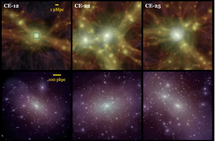
The range of cluster morphologies in our suite, on both large and small scales, is illustrated by Fig.2. For three clusters, this figure shows the gas density and temperature as in Fig.1, projected within a cube of 30 pMpc side length (top row), and in the bottom row the stellar mass surface density (grey scale) blended with the gas density (purple through yellow) within a cube of 2.5 pMpc side

length. Both are centred on the potential minimum of the cluster. For guidance, the region depicted in the bottom row is indicated by the green box in the top left panel.

Figure 2. Three visual examples of the variety of clusters in the mass range 4×1014_M

–1.4×1015_M

in the Hydrangea suite at redshiftz=0. The top row shows the projected gas density in a 30 pMpc cube with colour indicating the gas temperature as in Fig.1. The bottom row shows the central 2.5 pMpc of each simulation, with stellar surface density in shades of grey overlaid on gas density (purple through yellow). The green box in the top left panel indicates the size of the regions depicted on the bottom row.

dominating ‘brightest cluster galaxy’ (BCG; e.g. CE-12 and CE-22), whereas CE-25 in the right-hand column is currently undergoing a triple merger without an obvious ‘central’ galaxy.7

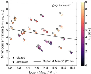
Fig. 3presents an overview of the distribution of the central C-EAGLE clusters in mass–concentration space, where concentra-tions c≡r200c/rswere obtained by fitting an NFW profile with scale radiusrsto the spherically averaged DM distribution between r=0.05 and 1r200c(Neto et al.2007; Schaller et al.2015b), centred on the potential minimum of the cluster. Clusters that are ‘relaxed’ (i.e. with an offset between the centre of mass and centre of poten-tial,s, less than 0.07r200cand a substructure fraction of less than 0.1; Neto et al.2007) are shown as circles, unrelaxed haloes that violate one or both of these criteria as stars. Clusters from the Hy-drangea sample (i.e. those with high-resolution regions extending to 10 r200c) are represented by filled symbols, the six remaining C-EAGLE clusters by open symbols. In qualitative agreement with the findings of e.g. Neto et al. (2007), unrelaxed clusters are typ-ically less concentrated than similarly massive relaxed ones. With significant scatter, the C-EAGLE clusters follow the well-known trend towards lower concentration at higher mass, consistent with the trend from the large DMO simulation in the Planck CDM cosmology of Dutton & Macci`o (2014).

7_{As can be seen in the top panel, this merger leads to an expansion of the} hot halo in a clear shock front.

We also indicate the formation time of each cluster, defined as the lookback time when the main progenitor of the cluster assembled half its present-day mass, as the colour of each point. As expected, there is a strong correlation between age and mass in the sense that less massive clusters assembled earlier. A second, albeit less strong, correlation exists between concentration and formation time (less concentrated clusters having typically formed somewhat more recently). In future work, we will exploit this diversity of our cluster sample to investigate in detail the impact of these differences on the galaxy population. TableA1in Appendix A lists the best-fitting concentrations along with other information on the mass, position, and environment of all the C-EAGLE clusters.

In combination, the 24 Hydrangea regions contain, atz=0 and within 10r200cfrom the centre of their main halo, 24 442 galaxies withMstar≥109M, and 7207 withMstar≥1010M. We note that this exceeds the corresponding numbers in the 100 cMpc EAGLE reference simulation by a factor of2.5, as a consequence of the larger (combined) simulation volume and the higher galaxy density in our simulated clusters.

3 S T E L L A R M A S S E S A N D Q U E N C H E D F R AC T I O N S O F S I M U L AT E D C L U S T E R G A L A X I E S

We begin our analysis of the Hydrangea simulations by compar-ing their predictions for two fundamental galaxy properties to

Figure 3. Mass–concentration relation of the C-EAGLE clusters at redshift

z= 0. The 24 Hydrangea clusters are shown as filled symbols, colour indicating the lookback time when the cluster assembled half its present-day mass,t1/2). The additional six clusters introduced by Barnes et al. (2017b) are shown as empty symbols. Concentration is defined asc ≡r200c/rs, wherersis the best-fitting NFW scale radius. Relaxed clusters are shown with circles, unrelaxed ones with star symbols (see the text for details). The sample spans a wide range in mass, concentration, dynamical state, and assembly histories.

observations, namely their stellar masses (Section 3.1), and quenched fractions (Section 3.2). We restrict ourselves to compar-isons to observations atz≈0, and will test the simulation predictions at higher redshift in future work. Because the observational studies, we are comparing to are focused on the central cluster regions, we include in this section also the six additional C-EAGLE clusters from Barnes et al. (2017b) whose high-resolution regions extend only to 5r200c.

3.1 Galaxy stellar masses

The stellar mass of a galaxy is one of its most fundamental char-acteristics, and many other properties have been shown to correlate strongly with stellar mass: e.g. colour, SFR (e.g. Kauffmann et al.

2003b; Wetzel et al.2012), metallicity (e.g. Tremonti et al.2004; Gallazzi et al.2005; S´anchez et al.2013), and, for centrals, their halo mass (e.g. White & Rees1978). We now test the galaxy masses predicted by our simulations against observations, for both central cluster galaxies (‘BCGs’) and their satellites.

3.1.1 BCG and halo stellar masses

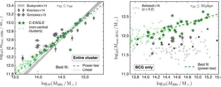
In Fig.4, we show both the total stellar mass of the clusters in our simulations (i.e. the mass of all star particles withinr3D=r500c, the radius within which the average density equals 500 times the critical density; left-hand panel), and the stellar mass of the BCG, i.e. the galaxy at the potential minimum of the cluster’s FoF halo, in the right-hand panel (integrated within a circular aperture withR2D=50 pkpc, see below). Both are shown as a function of total halo mass, which is quantified asM500cin the left-hand panel, but asM200cin the right-hand panel. Predictions from our simulations are shown in shades of green, dark for the 30 central clusters (i.e. the most massive ones in their simulation volume), and light green for oth-ers. Observational data are show in grey. For halo stellar masses, we

compare to the observations of Gonzalez et al. (2013) and Kravtsov, Vikhlinin & Meshscheryakov (2014), and the best-fitting relation derived from SDSS images by Budzynski et al. (2014). In the obser-vations,M500cis estimated from the X-ray temperature (Gonzalez et al.2013; Kravtsov et al.2014) and the mass-richness relation (Budzynski et al.2014); we multiply these with a factor of 1.5 to convert fromM500ctoM200c. In the simulations, we measure halo masses directly (masses derived from mock X-ray spectra are pre-sented in Barnes et al.2017b). All measurements of the total stellar mass in the halo in the left-hand panel include contributions from intracluster light, in both the simulations and observations. We note that the first two observational data sets are from clusters atz 0.1, whereas the Budzynski et al. (2014) relation was derived for clusters at 0.15≤z≤0.4. We here compare to the simulation output atz=0.101 as a compromise between these two ranges.

We first consider the simulation prediction for the 30 central clusters (dark green stars in Fig. 4), which exhibit a fairly tight relation between halo mass and both the halo and BCG stellar mass. The former is slightly sublinear (best-fitting power law in-dexα=0.86±0.05, with a best-fitting overall stellar fraction of 1.51 per cent). This is less steep than the relation of Budzynski et al. (2014),α=1.05±0.05, but slightly steeper than in Gonzalez et al. (2013) and Kravtsov et al. (2014). A sublinear scaling between the stellar and halo mass of galaxy clusters was also reported by Andreon (2010). We therefore conclude that, overall, the (central) C-EAGLE clusters have formed approximately realistic amounts of stellar mass (see also Barnes et al.2017b).

The agreement is less good when only the stellar mass of the BCG is considered, which we define as the mass within a (2D) radial aperture of 50 pkpc and integrating through the entire high-resolution simulation region along the line of sight (right-hand panel of Fig.4). Stott et al. (2010) have shown that this aperture mimics the Kron (1980) aperture commonly encountered in observational analyses, including that of Bellstedt et al. (2016) whose BCG stellar mass measurements (atz<0.2, and including the measurements of Lidman et al. 2012 used by these authors) we show as light grey circles. Also shown are BCG masses from Kravtsov et al. (2014), measured within a projected radius of 50 pkpc, and those of Gonzalez et al. (2013), corrected toR2D≤50 pkpc by multiplying with a correction factor of 0.4 (see Gonzalez, Zabludoff & Zaritsky

2005).

Figure 4. Left:stellar mass of C-EAGLE clusters withinr500c (green stars) as a function of true halo mass, compared to several observational data sets (grey points and band). Large dark green symbols represent the 30 central clusters within each simulation, other clusters within the simulation volume (with

M200c≥5×1013M) are shown as small light green stars.Right:stellar mass of the simulated BCGs as a function of halo mass, measured within a circular aperture ofR2D<50 pkpc, compared to observations. In both panels, dashed dark green lines show the best power-law fit to the simulated relation for central clusters with slopes ofα=0.86±0.05 (withinr500c) andα=0.41±0.06 (for the BCGs); thin light green lines show the analogous fits for non-central clusters. In the left-hand panel, the dotted dark green line additionally shows the best linear fit, corresponding to a stellar fraction of 1.51 per cent. Although the total mass of stars in the halo (withinr500c) is reproduced well by the simulations, BCGs are too massive by a factor of∼3. Non-central (‘secondary’) clusters follow the same relation as their central counterparts.

Unrealistically massive central cluster galaxies have also been a common feature of many previous simulations. In the earliest cases, this was a consequence of including no feedback, or only stellar feedback which becomes ineffective at regulating star for-mation in haloes aboveM200c≈1012M(see Balogh et al.2001 and references therein). During the last decade, these discrepan-cies have motivated the inclusion of AGN feedback in simulations, which alleviates this ‘overcooling problem’ in groups and clusters (e.g. Sijacki et al.2007; Fabjan et al.2010; McCarthy et al.2010; Gaspari, Brighenti & Ruszkowski2013), primarily by expelling gas from their progenitors atz≈2–4 (McCarthy et al.2011). However, in line with our findings from Fig.4, a number of studies in recent years have shown that even the inclusion of AGN feedback models can still lead to predicted present-day SFRs, stellar masses, and hot gas fractions of massive haloes that are higher than observed (e.g. Fabjan et al.2010; Ragone-Figueroa et al.2013; Vogelsberger et al.

2014; Schaye et al.2015; see also Scannapieco et al.2012). It is likely that the resolution of this longstanding problem will require the development of less simplistic AGN feedback models that are more efficient at expelling gas from massive haloes at high redshift. To judge the effect of overly massive BCGs on the predicted re-lation between stellar mass withinr500candM500c(left-hand panel), we have also computed cluster stellar masses excluding a sphere of radius 50 pkpc around the cluster centre (for clarity, this is not shown in Fig. 4). Because the relation between BCG mass and halo mass is strongly sublinear (see right-hand panel of Fig.4), this correction does not affect clusters withM500c>1014.4M. In lower-mass clusters, excluding the centre completely – which is clearly an overcorrection, since the C-EAGLE BCG masses at the low-mass end are only too high by a factor of∼2 – reduces the stellar mass by up to 0.2 dex and shifts the C-EAGLE predictions on the relation of Budzynski et al. (2014). On a qualitative level, the excess mass in our simulated BCGs does therefore not affect our conclusion that the total stellar mass in the C-EAGLE clusters is consistent with observations.

Due to their large volume, the Hydrangea simulations also contain a large number of ‘secondary’ cluster haloes that are less massive than the ‘primary’ one at the centre of each simulation. In total, there are 38 of these withM200c>5×1013Mwithin 10 (5)r200cfrom the central cluster in the Hydrangea (other C-EAGLE) simulations. This number is boosted to 81 when including objects beyond this nominal edge of the high-resolution sphere, but which are still far away (>8 pMpc) from any low-resolution boundary particles.8_At fixedM500c, secondary clusters (light green stars in Fig.4) contain the same stellar mass as primaries, both withinr500cand in their BCG.

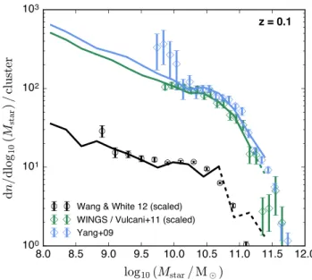
3.1.2 The stellar mass function of satellite galaxies

We now compare the simulation predictions for the low-redshift satellite GSMF. This has been studied observationally by several authors in recent years, including Yang et al. (2009, based on SDSS spectroscopic data and the Yang et al.2007SDSS halo catalogue), Vulcani et al. (2011, from the WINGS survey of nearby galaxy clusters), and Wang & White (2012, again from SDSS data but stacking galaxy counts around bright isolated galaxies).

All three of these observational studies exclude BCGs, but each uses a somewhat different definition of ‘satellite galaxy’. We there-fore begin by briefly describing these different selections and our methods for approximating them within the C-EAGLE simulations. Yang et al. (2009) used the Yang et al. (2007) halo catalogue to match SDSS galaxies to underlying DM haloes based on their spatial distribution. The most massive galaxy in each halo is

8_{These ‘external’ secondary clusters can exist because the high-resolution} regions atz≈0 are, in general, non-spherical. We have verified that they do not display any significant difference in their stellar masses from secondary clusters within the nominal high-resolution region.

identified as ‘central’, while all others are ‘satellites’. These au-thors report the satellite GSMF for different bins of halo mass, out of which we here compare to the (most massive) bin with 14.4≤log10M200c/(h−1M)<14.7. There are seven C-EAGLE clusters in this mass range, for which we select all simulated galax-ies thatSUBFINDidentifies as satellites of the cluster FoF halo.

Vulcani et al. (2011) assigned cluster membership in the WINGS catalogue (Fasano et al. 2006) based on 2D projected distance from the cluster centre (R2D≤0.6r200). The WINGS clusters have

M200c1014.5M(Fasano et al.2006).9We therefore compare to the 17 C-EAGLE clusters withM200c≥1014.5Mand select those galaxies withinR2D≤0.6r200cfrom the potential minimum of each cluster.10

Wang & White (2012) used a fixed 300 pkpc aperture around bright isolated galaxies to count satellites, but even in their highest stellar mass bin, the typical halo mass (as estimated from semi-analytic models) is only∼1013.7_M

. This is slightly lower than the halo mass range of our simulations, so we compare to simu-lated haloes in the mass range 14.0≤log₁₀M200c/M<14.5 (13 clusters) and re-normalize the Wang & White (2012) GSMF as described below.

Besides differences in galaxy selection, the observations span a range of redshifts, with medianz≈0.1 for SDSS (Yang et al.

2009; Wang & White 2012), while the WINGS clusters lie at 0.04< z < 0.07 (Vulcani et al.2011). For simplicity, we com-pare all three data sets to the simulation predictions atz=0.101, but have verified that differences to the predictions atz= 0 are small. In all three cases, we compute stellar masses in the simu-lations as the sum of all gravitationally bound star particles that are within 30 pkpc from the potential minimum of their subhalo. Schaye et al. (2015) have shown that this aperture yields a good match to the Petrosian apertures often employed in observations, including those from the SDSS. We restrict our comparison here to the primary (central) clusters of each simulation.

The comparison between simulations and observational data is shown in Fig.5. The simulated GSMF is shown with solid lines where bins contain more than 10 galaxies, and dashed lines for more sparsely sampled bins at the high stellar mass end. The obser-vations are shown as empty symbols, with error bars indicating the observational 1σuncertainties. Data points for WINGS (green) and Wang & White (2012) have been scaled by multiplying their stellar mass function with a correction factor such that the total number of galaxies above a given threshold (Mstar=109.8Mfor WINGS, 109.4_M

for Wang & White2012) is the same as in the C-EAGLE simulations. In the case of WINGS, this is necessary because the GSMF presented by Vulcani et al. (2011) has been scaled for the purpose of comparing to field galaxies, while the GSMF of Wang & White (2012) was derived for haloes that are less massive than the C-EAGLE sample (see above); the correction factor applied to this data set is equal to 1.50. Differently coloured lines correspond to simulated GSMFs matched to the correspondingly coloured ob-servational data set, as described above.

9_{We have used theLX–M}

500crelation of Vikhlinin et al. (2009) to convert the WINGS X-ray luminosities of Fasano et al. (2006) to halo masses, with an additional correction factor of 1.5 to convert toM200c.

10_{We have not imposed an additional cut along the line of sight, because the} criterion ofz≤3σ(with redshiftzand cluster velocity dispersionσ) of Vulcani et al. (2011) corresponds to an integration length that is comparable to the size of the high-resolution region in our simulations.

Figure 5. Galaxy stellar mass function (GSMF) atz=0.101 for satellites in the C-EAGLE simulations (solid lines, dashed where there are<10 galaxies per 0.25 dex bin) compared to observations (open diamonds). The three dif-ferent lines represent galaxy selections approximately matched to the respec-tively coloured observational survey: 14.0≤log10(M200c/M)<14.5,

R2D<300 pkpc (black); 14.5≤log10(M200c/M),R2D<0.6r200c(green); 14.4≤log10M200c/(Mh−1)<14.7, all halo members (blue). Overall, the simulations achieve an excellent match to the observations.

Overall, the simulatedz≈0 GSMF agrees well with all three data sets. The only slight tension is seen at the low-mass end of the Wang & White (2012) and Yang et al. (2009) comparisons, where the observations hint at an upturn of the GSMF that is not seen in the simulations. We note that these observational data points also have large uncertainties – in the case of Yang et al. (2009), the discrepancy for an individual data point is only significant at the ∼1σlevel – but alternatively, this deficiency might be a consequence of overly efficient star formation quenching in low-mass galaxies in our simulations, as we shall discuss shortly.

The accuracy of the predicted cluster GSMF reflects, in part, the calibrated match between the EAGLE simulations and the field GSMF (Schaye et al.2015). However, as shown below, there are significant differences between the field and cluster GSMF in our simulations. The close agreement between our cluster GSMF and the observations shown in Fig.5therefore suggests a realistic mod-elling of cluster-specific aspects of galaxy formation, at least to the extent that they manifest themselves in the stellar mass of galax-ies. We exploit this success of our simulations further in Section 4, where we compare the GSMF in and around simulated clusters to the field.

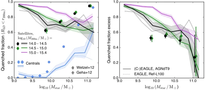
3.2 Satellite quenched fractions

A second key property of galaxies, which is closely related to their stellar mass, is their SFR. Observations have shown conclusively that galaxies in dense environments are biased towards lower spe-cific star formation rates (sSFR≡SFR/Mstar; e.g. Kauffmann et al.

Figure 6. Left:quenched satellite fraction withinr3D≤r200m, in bins of cluster mass (differently coloured solid lines) as a function of stellar mass. The blue solid line shows the corresponding trend in the field, i.e. centrals in the AGNdT9-L050 simulation from the EAGLE suite. Shaded bands indicate 1σ binomial uncertainties (Cameron2011). The dotted blue and black lines are the corresponding trends from the EAGLE Ref-L100 simulation. Filled circles with error bars show the corresponding values from the SDSS DR7 analysis of Wetzel et al. (2012) and blue diamonds the observed quenched fractions of field dwarfs from Geha et al. (2012). In agreement with observations, simulated satellites show an enhanced quenched fraction compared to the field, albeit with discrepancies in the trends withMstar(see the text for details).Right:the satellite quenched fraction excess, (fqsat−fqcen)/(1−fqcen), which shows quantitative

agreement between simulations and observations atMstar>1010M.

In the left-hand panel of Fig.6, we show the passive fraction of C-EAGLE cluster satellites as a function of stellar mass and host mass. For consistency with the observational analysis of Wetzel et al. (2012), we define ‘passive’ galaxies as those with sSFR<10−11 yr−1_{. For the same reason, we take cluster mass here asM}

200m(the mass within the radiusr200m inside which the average density is 200 times themean, as opposed to critical, density of the Universe) and select as satellites those galaxies at radiir3D≤r200m(excluding the BCG).11

Clusters are grouped into three mass bins betweenM200m=1014 and 1015.5_M

, represented by different colours. For comparison, we also show the corresponding quenched fraction of central galax-ies from the EAGLE AGNdT9-L050 simulation (which was run with the exact same simulation parameters as C-EAGLE; solid blue line). Shaded bands indicate the statistical binomial 1σ uncertainty (Cameron2011) on the quenched fraction. Observational data from Wetzel et al. (2012) are overlaid as filled circles in correspond-ing colours; the error bars represent 1σuncertainties. We note that their observations do not probe the highest halo mass bin (purple). Also plotted are the quenched fractions of low-mass field galax-ies from Geha et al. (2012, blue diamonds). Finally, the analogous trends from the EAGLE Ref-L100 simulation – whose parame-ters describing AGN feedback are different from C-EAGLE, see Section 2.1 – are shown as dotted lines, both for centrals (blue) and the lowest-mass cluster bin (black).

The dominant feature of Fig.6is an increased quenched frac-tion of satellites across the range of halo masses shown here (M200m > 1014M), at least at Mstar <1011M, which agrees

11_{The group finding algorithm of Wetzel et al. (2012) accounts for} line-of-sight projection in a probabilistic way, with the aim of assigning galaxies to haloes in 3D space. We have repeated the analysis presented here with a cut inR2Dinstead, and found no qualitative differences.

qualitatively with observations. Similar to what is seen in the Wetzel et al. (2012) data, the quenched fractions in the 14.0–14.5 and 14.5–15.0 halo mass bins (black/green) closely follow each other. For the nine clusters withM200m > 1015M, the simula-tions predict a substantially higher quenched fraction, especially at intermediate stellar masses (Mstar≈1010M).

In contrast both to observations and to simulated central galaxies, the quenched fractions of simulated cluster satellites do not show an increase with stellar mass. On the contrary, they show a decrease, especially atMstar1010M. The quenched satellite fraction in the C-EAGLE simulations atMstar 1010Mis therefore lower than observed. This discrepancy is most severe for the most mas-sive galaxies (Mstar≈1011.5M; 70 per cent in C-EAGLE versus near 100 per cent in the data). We point out, however, that even for centralgalaxies, in both the EAGLE AGNdT9 and Ref runs (blue solid and dotted lines), the massive quenched fractions are under-predicted, which points to a more fundamental discrepancy between the simulations and observations, for example because quenching due to internal mechanisms such as AGN (see e.g. Bower et al.

2017) is not efficient enough in the EAGLE model. Alternatively, the quenched fractions in the observations may be overestimated, as demonstrated by Trayford et al. (2017) in the case of quenched fractions derived from galaxy colours. However, the quenched frac-tions of Wetzel et al. (2012) are derived from optical spectra and not colours, and a recent study by Chang et al. (2015) found that these tend tooverestimate SFRs, which would exacerbate rather than alleviate the discrepancy. To isolate theenvironmentalimpact on the quenched fraction, we plot in the right-hand panel of Fig.6

the ‘quenched fraction excess’, defined as (fsat

q −fqcen)/(1−fqcen) as proposed by Wetzel et al. (2012). In this metric, the simulations show much closer agreement with the observations, indicating that the environmental impact on star-forming gas is modelled correctly in our simulations, at least forMstar>1010M.

At lower stellar masses (Mstar 1010M), observations indi-cate a continued decrease in the passive fraction of both satel-lites and centrals with decreasing stellar mass (Geha et al.2012, blue diamonds in Fig.6). While this is approximately reproduced by EAGLE centrals – whose passive fraction is<10 per cent at Mstar=109M– the passive fraction of satellites in our simulations

increasessignificantly, and almost reaches unity atMstar=109M, independent of host mass. In Schaye et al. (2015), it was already shown that EAGLE predicts a passive fraction in the combined galaxy population (centrals and satellites) that rises towards lower stellar masses belowMstar≈109.5M, and that this effect is strongly resolution dependent. Because almost all these quenched low-mass galaxies are satellites (at least down toMstar = 109M, see our Fig.6), the overefficient quenching of low-mass satellites in C-EAGLE can therefore also be primarily ascribed to resolution ef-fects, even though all galaxies shown here are resolved by1000 particles.

We speculate that this effect may be connected to the overly porous structure of atomic hydrogen discs in many EAGLE galax-ies reported by Bah´e et al. (2016). As a consequence of limited resolution, star formation feedback events in the EAGLE model create holes that are larger than observed, and it is possible that this increased porosity might make the disc more susceptible to being stripped under the influence of ram pressure.

As a final note, we emphasize that an artificial increase in the pas-sive (or red) fraction of low-mass satellites with decreasing stellar mass is not unique to our simulations, and has also been described by many other authors. This includes hydrodynamical simulations with a fundamentally different treatment of hydrodynamics and stellar feedback (Vogelsberger et al.2014) as well as semi-analytic models (e.g. Guo et al.2013; Henriques et al.2013). As well as improved resolution and more sophisticated feedback recipes, the generation of low-mass satellite galaxies with realistically low quenched frac-tions may therefore also require other changes to the simulation model, e.g. in the treatment of the star-forming interstellar medium (ISM).

4 E N V I R O N M E N TA L I N F L U E N C E O N S T E L L A R M A S S E S

We have shown in the previous section that the C-EAGLE simula-tions produce realistic satellite galaxy stellar mass distribusimula-tions in the cores of massive clusters, while the underlying EAGLE model reproduces, by construction, the GSMF in the field (Schaye et al.

2015; Crain et al.2015). This gives the simulations power to gain theoretical insight into how environment affects the GSMF in and around clusters. We will now proceed with a first analysis of these environmental effects. For consistency with the previous section and SDSS-based observations (see Schaye et al.2015), we continue to only consider stars within 30 pkpc from the potential minimum of each galaxy’s subhalo. Despite some difference in detail, none of our findings below change qualitatively when including all stars bound to the subhalo instead.

4.1 Environmental impact on the normalized stellar mass function

A key difficulty of comparing GSMFs between different environ-ments is the application of a suitable normalization, since by def-inition the overall density of galaxies is higher in clusters than in the field. In the observational literature this has, for instance, been accomplished by re-normalizing cluster and field mass functions so both yield the same total number of galaxies above a given mass

limit (e.g. Vulcani et al. 2011). In our simulations, a more natu-ral way to accomplish this is to divide the number of galaxies by thetotal masswithin the same volume, effectively computing the bias of galaxies of different mass with respect to the general mass distribution as in Crain et al. (2009).

We present this comparison in Fig.7, where we show the nor-malized GSMF, i.e.φ≡dn/d log10Mstar/(Mtot/1010M), where

Mtotis the total mass within the volume that galaxies are selected from. We distinguish between Hydrangea clusters in three different mass bins (different panels, increasing from left to right). For each bin, we stack all clusters and extract the GSMF in three concentric shells centred on the cluster’s potential minimum, in the radial range r=0–r200c(the virialized central region), 1–5r200c(the region com-prising a mix of first-infall and backsplash galaxies; see Bah´e et al.

2013), and 5–10r200c(the primordial infall region). For comparison, we also show the normalized GSMF from the EAGLE AGNdT9-L050 (blue) and Ref-L100 (purple) periodic-box simulations. Since these model representative cosmic volumes, they can be taken as estimates of the ‘field’ GSMF. There is very close agreement be-tween these latter two distributions (Schaye et al.2015), with the key difference being that Ref-L100 extends to higher masses due to its eight times larger volume.

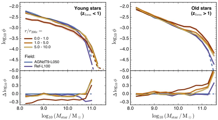
At first sight, the normalized stellar mass function shows lit-tle difference between the different environments, with particularly close agreement atMstar ≈ 1010M in all three halo mass bins. On closer inspection, however, there are two clear and significant differences. First, there is a deficiency of low stellar mass galaxies (Mstar1010M) withinr200c(red line), of up to∼0.2 dex. Sec-ondly, massive galaxies (Mstar1010.5M) are more numerous in our simulated clusters, from the central region (<r200c) to the far out-skirts (the 5–10r200czone; yellow). Qualitatively, this is consistent with the recent Dark Energy Survey analysis of Etherington et al. (2017), who found a higher fraction of massive galaxies in higher density environments. The bottom panels show the mass functions normalized to Ref-L100 to bring out these differences more clearly. Over more than a decade in halo mass, the environmental differ-ences in galaxy stellar mass show no strong dependence on cluster mass.

The deficiency of low-mass galaxies within the virial radius can be due to tidal stripping (or even complete disruption) of satellites, lack of stellar mass growth as a result of star formation quenching, or a combination thereof. In Fig. 8, we test these hypotheses by constructing GSMFs separately for young and old stars, defined as those formed after or before redshiftz=1, respectively. The en-vironmental impact on these two different populations is strikingly different. From the left-hand panel, the young stellar mass function shows a strong deficiency at the low-mass end (by up to 0.4 dex), but only a minor high-mass excess except for the most massive galax-ies (Mstar,young>1011M). From the horizontal offset between the curves, stellar stripping would have to reduce the young stellar mass of anMstar,young=1010Mgalaxy by∼0.3 dex to account for this offset. However, we will show in a forthcoming paper that stellar stripping withinr200chas a typical effect of<0.1 dex at these mass scales and can therefore not be a significant contributor to the lack of young stars withinr200c.

In contrast, galaxies with a given mass in old stars down to ∼108_M

Figure 7. Top row:galaxy stellar mass function (GSMF) normalized to the total mass within the respective volume,φ≡dn/d log10Mstar/(Mtot/1010M). Individual columns contain clusters of differentM200c(as indicated in the top right corner). Differently coloured lines (dashed where there are less than 10 galaxies per 0.25 dex bin) represent different radial zones in each cluster: insider200c(red); between 1 and 5r200c(i.e. the region containing a population of backsplash galaxies, orange); the far outskirts beyond 5r200c(yellow). For comparison, the mass functions from the AGNdT9-L050 (blue) and Ref-L100 (purple) EAGLE runs are also shown.Bottom row:logarithmic ratio between each GSMF and that from the Ref-L100 periodic box. All halo mass bins show an excess of massive galaxies in and around clusters, without a clear radial trend. Galaxies less massive than∼1010_M

, on the other hand, are deficient in the central cluster regions (red).

Figure 8. Top panels:the normalizedz=0 galaxy stellar mass function (GSMF)φ≡dn/d log10Mstar/(Mtot/1010M) split by stellar formation redshift into ‘young’ stars (zform<1.0, left-hand panel) and ‘old’ stars (zform>1.0, right-hand panel). As in Fig.7, the Hydrangea volumes are split into three radial zones (red, orange, and yellow lines) and compared to the EAGLE periodic-box simulations (blue/purple); dashed lines indicate bins with fewer than 10 galaxies. The shaded band, shown only forr<r200c(red) for clarity, indicates the Poisson uncertainty on the GSMF. For clarity, thebottom panelsshow the logarithmic ratio between each GSMF and that from the AGNdT9-L050 periodic box. Evidently, the deficiency at low mass and excess of stellar mass at high mass are due to two different processes, since the former only affects young, and the latter mostly old stars.