Schutt_unc_0153M_15843.pdf

A VALIDATION OF STABILITY-BASED ESTIMATES OF NORTH CAROLINA’S OFFSHORE WIND RESOURCE USING A NESTED BOUNDARY LAYER METHOD

Megan Schutt

A thesis submitted to the faculty at the University of North Carolina at Chapel Hill in partial fulfillment of the requirements for the degree of Masters of Science in the Marine Science

Department in the College of Arts and Sciences.

Chapel Hill 2016

A

Megan Schutt: A validation of stability-based estimates of North Carolina’s offshore wind resource using a nested boundary layer method

(Under the direction of Harvey Seim)

A

This study could never have been seen to completion without the aid of many. Foremost is my advisor, Harvey Seim, whose contributions both academic in nature and those that come with simply being an esteemable human being, are countless. Thank you, Harvey, for providing a place to learn for this engineer adrift. Your guidance, support, and good humor made for a lovely three years, and they will not be forgotten.

T

C

LIST OF FIGURES ... VII

LIST OF ABBREVIATIONS ... IX

INTRODUCTION ...1

PAST WORK AND MOTIVATION ... 2

NC Wind Study Background ... 2

THEORY ... 3

MOST ... 3

COARE 3.0 ... 5

CURRENT MOTIVATIONS ... 6

METHODS ...8

LOCATION AND DATA SOURCES ... 8

Geography ... 8

SODAR ... 9

Offshore Buoys ... 10

Other Ancillary Data ... 11

Data Input Process ... 12

INTERNAL BOUNDARY LAYER ALGORITHM ... 12

RIBL Height Estimation ... 14

TIBL Height Estimation ... 16

CASE IDENTIFICATION ... 18

Constraints ... 20

Stability Characterization ... 22

RESULTS ... 24

DIFFERENCES IN VERTICAL VARIATIONS IN THE HORIZONTAL WIND SPEED PROFILE ... 24

Roughness-based effects ... 25

Stability effects ... 26

MODEL DEVELOPMENT ... 27

The neutral model ... 28

Including a stability parameter ... 29

MODEL IMPROVEMENT BASED ON STABILITY ... 30

TURBULENCE MEASUREMENTS ... 34

DISCUSSION ... 37

EXAMPLES UNDER CONSIDERATION ... 37

Unstable ocean case: ... 37

Thermal influences over the sound: ... 40

TURBULENCE ... 42

WIND SHEAR ... 45

SUMMARY OF MODEL ESTIMATION ... 47

CONCLUSIONS ... 51

L

F

FIGURE 1:IMPACT OF STABILITY ON THE WIND PROFILE ... 5

FIGURE 3:GULF STREAM,MAB AND SAB WATERS ... 9

FIGURE 4:SODAR ... 10

FIGURE 2:ORIENTATION ... 10

FIGURE 5:RALEIGH BAY BUOY ... 11

FIGURE 6:PROCESS FLOW OF DATA INPUT ... 12

FIGURE 7:INTERNAL BOUNDARY LAYERS ... 14

FIGURE 8:ROUGHNESS ELEMENTS OF HATTERAS ISLAND ... 15

FIGURE 9:SATELLITE SST MEASUREMENTS FROM RUTGERS COOL ... 17

FIGURE 10:REGRESSION METHOD... 20

FIGURE 11:SOUND AND OCEAN DIRECTIONAL DEFINITION ... 21

TABLE 1:CASES IDENTIFIED ... 23

FIGURE 12:OCEAN AND SOUND CASE WIND PROFILES ... 25

FIGURE 13:OCEAN (A)AND SOUND (B) WINTER STABILITY DEPENDENT CHANGES ... 26

FIGURE 14:SOUND CASE WITH A NEUTRAL (A) AND STABILITY-BASED MODEL (B) ... 28

FIGURE 15:OCEAN CASE - NEUTRAL (A) AND STABILITY-BASED (B) MODEL ... 30

FIGURE 16:MEAN WIND SPEED ESTIMATIONS ... 31

FIGURE 17:RMS ... 33

FIGURE 18:IMPROVEMENT OF RMS ... 34

FIGURE 19:OCEAN AUTUMN AND OCEAN WINTER SEASONAL DEPENDENCE ... 36

FIGURE 20:UNSTABLE MODEL EXAMPLE ... 37

FIGURE 21:OSU1SSTIMAGE ... 38

FIGURE 23:PAMLICO SOUND SURFACE LAYER EVOLUTION ... 41

FIGURE 24:OCEAN TURBULENCE PROFILES ... 42

FIGURE 25:SOUND TURBULENCE PROFILES ... 43

FIGURE 26:SHEAR COMPARISON OF OCEAN CASES (A),SOUND CASES,(B) ... 46

TABLE 2:MEAN WIND SPEED AND WIND SHEAR DIFFERENCES ... 47

L

A

COARE Coupled Ocean-Atmosphere Response Experiment COOL Coastal Ocean Observation Lab

IBL Internal boundary layer MAB Mid-Atlantic Bight

MOST Monin-Obukhov similarity theory

NC North Carolina

NDBC National Data Buoy Center

RIBL Roughness internal boundary layer SAB South Atlantic Bight

SAT Surface air temperature SODAR Sonic Detection and Ranging SST Sea surface temperature

I

One way for renewable energy to become cost competitive with current fossil fuel sources is continued upscaling of wind turbine size (Lantz, Wiser, & Hand, 2012). Advancements of this nature, common to deployments offshore, require increased knowledge of wind speed at higher turbine heights. Further, overall improvement of the characterization and estimation of the available resource would benefit offshore wind farms of any size (Klaassen, Miketa, Larsen, & Sundqvist, 2005). The ABL has been thoroughly investigated historically in the Great Plains region (Businger, Wyngaard, Izumi, & Bradley, 1971). However, the wind climates of coastal and offshore areas lack the observations and validating experiments, and often consist of significantly different environmental conditions than that of land-based systems (Holtslag, Bierbooms, & van Bussel, 2015).

profiles measured by the SODAR will be used to verify a stability-based estimate of the offshore wind resource in North Carolina.

P

W

M

NCWIND STUDY BACKGROUND

An initial wind resource assessment of coastal North Carolina, prepared for the North Carolina General Assembly in 2009 (UNC, 2009) examined the feasibility of offshore wind energy development in the region. In conjunction with use conflict investigation in the area, geologic surveys, and an effort to improve the local regulatory hurdles, locations of prime potential were identified and presented to the assembly. The wind power estimation facet of this project used historical near surface wind speed measurements to assess the available wind resource, collected from a variety of airports, weather masts, and offshore buoys, and towers, most of which provided a measurement at less than 20 meters in height. A vertical extrapolation assuming steady, neutrally-stable, homogeneous conditions was used of the power law form:

𝑢(𝑧) = 𝑢𝑟𝑒𝑓( 𝑧 𝑧𝑟𝑒𝑓)

𝛼

where the free parameter, α, was empirically determined using several data sources, yielding a range of values. In the height extrapolation for coastal winds, this parameter was held constant on the lower end of this range, befitting the results from the oceanic based data sources.

Thomas, Seim, & Haines (2015) more recently have used surface wind measurements from satellite products to extend the assessment offshore, as well as compare stability-based corrections to the estimations of wind at 80m height. In comparison to the neutrally stable reference scheme, significant differences in wind speed at height were found, largely under stable atmospheric conditions. Thus, atmospheric stability has been investigated in the region, but no validation of stability-impacted profiles had been attempted. Wind profile measurements could provide the necessary corroboration of this method. The results gained from this project could be enough to both verify if and when the method is reasonable for this region, as well as ascertain whether any improvements could be made for specific locations or seasons.

T

MOST

The Monin-Obukhov similarity theory (MOST) states that in a horizontally homogeneous surface layer with quasistationary flow, only one dimensionless combination of the four independent variables affecting the flow can be formed – most often using the dimensionless buoyancy parameter, 𝜁 defined as

𝜁 =𝑧 𝐿

where 𝑧 is the height above the surface, and 𝐿 is the Obukhov length scale. 𝐿 is a function of heat flux at the surface as

𝐿 = − 𝑢∗ 3

𝜅 (_𝑇𝑔 0) (

𝐻₀ 𝜌𝑐_𝑝)

dynamic turbulence.’ This length scale can be taken as a height above which atmospheric stability influences the sublayer, or the thickness of the layer where dynamics (shear) dominate (Arya, 2001). The wind profile as a function of height and stability can then be approximated by a typical log-layer (depending on the friction velocity, von Karman constant, height, 𝐿, and an aerodynamic roughness length: 𝑧₀) of the form:

𝑢(𝑧) =𝑢∗ 𝜅 [𝑙𝑛

𝑧

𝑧₀− 𝜓 𝑚(𝜁)]

where the 𝜓_𝑚 function is defined for specific domains in Foken (2008) as

𝜓𝑚(𝜁) = 𝑙𝑛 [(1+((1−19.3𝜁)

1/4₎2

2 ) (

1+(1−19.3𝜁)1/4

2 )

2

] − 2𝑎𝑟𝑐𝑡𝑎𝑛((1 − 19.3𝜁)1/4_{) +}𝜋

2 for 𝑧 𝐿< 0

𝜓𝑚(𝜁) = −6𝜁 for 𝑧_𝐿≥ 0

It can easily be seen that for 𝑧

𝐿→ 0, 𝜓𝑚→ 0, and an asymptotic behavior is reached for near

neutral stratification. Additionally, the most dramatic changes in wind speed with height come with stable (positive values of) 𝑧

𝐿, with the negative domain of 𝐿 and its associated function yielding

COARE3.0

Direct measurement of all of the terms within the parameterization of 𝐿 remains difficult. The Coupled Ocean-Atmosphere Response Experiment (COARE) bulk algorithm was developed as a tool to quantify the turbulent and radiative fluxes in the tropical waters of the open ocean (Webster, & Lukas, 1992), and calculate values for a variety of parameters necessary for prediction of a near surface wind profile and surface flux conditions. It has undergone several documented improvements, and is currently used in this project in its 3.0 version (Fairall, Bradley, Hare, Grachev, & Edson, 2003). COARE uses measurements of wind speed, temperature and specific humidity of the air and water, and air pressure to iteratively solve the bulk flux relations

FIGURE 1:IMPACT OF STABILITY ON THE WIND PROFILE

the parameters relevant to the wind profile - friction velocity, 𝑢_∗, roughness length, 𝑧₀, and MOS length, 𝐿.

C

M

Validation of the COARE implementation of MOST used by Thomas et al. (2015) to make improvements to UNC (2009) requires highly resolved measurements of wind profiles, as well as knowledge of meteorological conditions in the surrounding environment. Confidence in MOST for wind-at-height estimation is essential not only for projects in this region, but also wind siting in oceanic areas in general. With the majority of early and formative studies in the discipline conducted in the American Great Plains (Businger et al., 1971, Great Plains Field Program, 1962, Kaimal, 1990), more attention must be paid to coastal and similarly dynamic environments to verify or adjust the empirically derived constants and functional forms. For example, recent studies in coastal areas of Northern Europe have found an underestimation in wind speed for various MOS derivations for near-neutral and stable stratification (Lange, Larsen, Hojstrup, & Barthelmie, 2004). It remains clear that in order to achieve the most accurate estimations of the available wind resource, a closer investigation into the applicability of methodologies must be undertaken.

M

L

D

S

GEOGRAPHY

The area of interest centers on Billy Mitchell Airport at Hatteras Island in North Carolina’s Outer Banks (see Figure 2). The airport is the location of the SODAR (SOnic Detection And Ranging), wind profiler and is bounded to the north and west by Pamlico Sound, a large body of water partially closed off from the open ocean by the various barrier islands of the Outer Banks. It is often of a relatively homogenous SST, especially as compared to the oceanic water on the other side of the islands. These Atlantic Ocean waters to the south and east of Hatteras Island are known for large horizontal temperature gradients at the sea surface. The western boundary current of the North Atlantic Gyre, the Gulf Stream, brings warm subtropical waters from lower latitudes north along the southeastern coast of America. Its shoreward edge is typically over the 400m isobath (Miller, 1994), and it breaks away from the continental shelf at Cape Hatteras.

by sea surface temperatures, a wind profile measurement here could provide an interesting opportunity to capture the effect of these dramatic changes in SST.

SODAR

The Scintec Flat Array SFAS SODAR (Figure 4) located at Billy Mitchell Airport (Figure 4) returns several useful measurements about the wind behavior at its location at half-hour time increments. Along with three-dimensional wind components, the dataset also includes vertical wind speed variance, 𝜎𝑤, and acoustic backscatter intensity, both of which can serve as measures

of the magnitude and type of turbulence in the atmosphere. All of these measurements are taken by the SODAR through a height range of 10-200 meters, at 5 meter increments. At some temporal

FIGURE 3:GULF STREAM,MAB AND SAB WATERS

and spatial intervals, measurements are not available because of power outages, inability of the SODAR to detect a complete vertical profile, or other inconsistencies.

OFFSHORE BUOYS

Two buoys were used to obtain measurements of both oceanic and meteorological properties. The buoy used principally is located in Raleigh Bay (RB),

to the south west of the SODAR, as seen in Figure 2. This buoy (Figure 5) is maintained by UNC-Chapel Hill/NCCOOS, and makes available measurements of wind speed, water and air temperature, air pressure, and humidity for use in the COARE 3.0 algorithm. It is typically located in the cooler coastal waters outside of the Gulf Stream. During times when the RB buoy was undergoing maintenance or had been decommissioned, the National Data Buoy Center Diamond Shoals (DS) buoy to the southeast of the SODAR site (Figure 4) served as the oceanic data source (air and water temperature, wind speed, air pressure, and dewpoint). The location of the DS buoy is sometimes within the colder shelf waters, and sometimes within a meandering eddy of warmer Gulf Stream waters. The water temperature measurement taken by each buoy reflect the presence of these different water masses, with water temperature sometimes spanning a ten to fifteen degree range within a 24 hour time interval. The dynamic nature of these temporal and

FIGURE 2:ORIENTATION

The location of study in the Outer Banks of North Carolina, marked with the various locations of data collection.

Stumpy Point Tower

FIGURE 4:SODAR

spatial gradients, as well as the differences between the locations of the two buoys in general could be an important factor in quantifying the atmospheric stability of the upwind conditions. A critical perspective should be retained when using the buoy data to characterize the stability of the wind profiles measured at Billy Mitchell, especially when the buoy used is not directly upstream of the wind measurement.

OTHER ANCILLARY DATA

If the wind direction indicated that the wind had come from over Pamlico Sound, the meteorological measurements from the buoys would be an inaccurate indicator of upwind conditions. In lieu of buoys, the sound cases make use of ancillary data sources from surrounding weather stations. The Coast Guard Station on Hatteras Island provides a water temperature measurement of Pamlico Sound (Figure 4). This

measurement was not available for part of 2013, so a water temperature measurement was obtained from the Oregon Inlet station instead. The Pamlico Sound weather mast maintained by Weatherflow, Inc. in the middle of the sound provides a wind speed and air temperature measurement, while the humidity measurement is obtained from Billy Mitchell airport. The Stumpy Point Tower (managed by Weather Flow) measures wind speed and air temperature at high temporal resolution at 95, 72, and 47m. The data from these stations and the buoys was measured as often as every minute. These values were averaged hourly in order to coincide with the measurements from the Billy Mitchell SODAR.

FIGURE 5:RALEIGH BAY BUOY

DATA INPUT PROCESS

As mentioned above, COARE uses wind speed, temperature and specific humidity of the air and water, and air pressure, a total of six environmental measurements required to quantify surface flux. The datasets detailed above are complexly intermittent. Some contain measurements that are more validly representative of upstream conditions, or measure more of the required COARE inputs, but they are not always available. A flowchart of prioritization is used for both sound and ocean cases to choose from available data (see Figure 6).

I

B

L

A

Knowledge of the growth of internal boundary layers (IBLs) is critical to relating wind profiles measured at the SODAR with the ancillary data collected from various locations in this coastal region. The two types of internal boundary layers investigated in this study are (1) those

FIGURE 6:PROCESS FLOW OF DATA INPUT

RIBLHEIGHT ESTIMATION

An algorithm for estimating the height a developing RIBL may reach after a step change in roughness was created using the relation from Stull, (1989) where 𝛿_{𝑅𝐼𝐵𝐿} is the height of the roughness internal boundary layer, 𝑧₀₁ is the aerodynamic roughness length of the first surface,

𝑧₀₂ is the aerodynamic roughness length of the second surface, and 𝑥 is the horizontal fetch over the second surface since the step change

𝛿_{𝑅𝐼𝐵𝐿} = 𝑧₀₁[0.75 + 0.03 ln (𝑧02 𝑧₀₁)] ∗ (

𝑥 𝑧₀₁)

0.8

where 𝑧₀₂> 𝑧₀₁. Roughness element values were obtained from a map of Hatteras Island created by TrueWinds AWS (Figure 8). The roughness elements that would be encountered at 5 degree directional intervals were tabulated, along with the fetch from that roughness element to the Billy Mitchell SODAR site. A variety of different processes were used with the relation above, and the

FIGURE 7:INTERNAL BOUNDARY LAYERS

The profiles measured by the Billy Mitchell SODAR on Cape Hatteras could be measuring the profiles of boundary layers associated with a variety of differing surfaces. In this visualization of developing IBLs, including the TIBL and RIBL possibly seen in the Ocean cases, it becomes clear that the growth rate of the IBL, and its resulting thickness by the time it is measured by the SODAR is an important parameter in identifying winds associated with an area away from the profile measurement.

Developing Stable TIBL

Unstable Thermal Layer Developing

most sensible results came from calculating the height using the maximum roughness element encountered as 𝑧₀₂ and its associated fetch. This method generally resulted in higher RIBL heights, on the order of 70-100 m for winds coming from the north, northeast, and west (usually associated with Sound cases), as compared to RIBL heights of 5-30 m for winds coming from the south and east (associated with Ocean cases). This result was to be expected given the fetches from these directions being a fraction of those associated with Sound cases. Any wind profile measured by the SODAR is only used for comparison purposes above this RIBL height, as the measurements below this RIBL height would be associated with a developing boundary layer over the land.

FIGURE 8:ROUGHNESS ELEMENTS OF HATTERAS ISLAND

Spatially determined aerodynamic roughness lengths surrounding Billy Mitchell Airport from AWS TrueWind. The maximum element encountered throughout the wind’s path was selected as the z0 parameter, along with its

TIBLHEIGHT ESTIMATION

In a similar fashion, an estimation of a thermal internal boundary layer growth can be made beginning at the clearly defined temperature gradients evident in the Gulf Stream boundary. An example of this boundary when it is clearly evidenced can be seen in Figure 9. The Gulf Stream SST is higher than that of the coastal waters, with a 4-5° temperature difference in this case. An upwind fetch was estimated in the direction of the wind speed as measured by the Billy Mitchell SODAR (also shown in Figure 9). The TIBL height, 𝛿_{𝑇𝐼𝐵𝐿}, was calculated with 𝑈: wind speed, 𝑇_𝑎: air temperature, 𝑥: downwind fetch, 𝛥𝑇: the step decrease in surface temperature, and 𝑔: gravitational acceleration, using an equation of the form (Garratt, 1992):

𝛿𝑇𝐼𝐵𝐿= 0.024𝑈√ 𝑇_𝑎𝑥 𝛥𝑇𝑔

These water temperatures match well with the SST image of the cooler coastal waters and the warmer signatures of the Gulf Stream, an indicator that within the span of this case, the COARE results are associated with differing bodies of water. While unstable TIBLs are not explicitly calculated for the case analysis that follows, they grow as:

𝛿_{𝑇𝐼𝐵𝐿}= 𝑎√𝑥

where 𝑎 is an empirical constant that ranges from 1.9-5 (Garratt, 1990). Even using the lower bound of the constant, unstable TIBLs associated with warmer Gulf Stream waters (the front is at minimum 20-30 km from shore at the lower edge of Hatteras Island) would always grow to a height

FIGURE 9:SATELLITE SST MEASUREMENTS FROM RUTGERS COOL

With this information, SODAR profile measurements can be divided into relevant layers applicable to the wind direction and stability regime. Environments classified as stable use wind measurements taken from the stable TIBL – most often within colder coastal waters, and under the stable TIBL height calculated from the Gulf Stream step change. Environments classified as unstable are more likely associated with the warmer Gulf Stream waters, upwind of the step change (decrease) in SST and above the calculated TIBL height. Wind profiles from the ocean direction and identified as unstable will be analyzed above this TIBL height, while those identified as stable will be compared with SODAR measurements below this height, and above the RIBL. For Pamlico Sound cases, a stable TIBL was calculated (pending data availability) from the change in near surface air temperature from the Stumpy Point Tower to the Pamlico Sound water mast. As unstable TIBLs are fast-growing, over the ~40 km fetch of Pamlico Sound, an unstable TIBL would grow to a height above the range of the SODAR.

C

I

FINDING TIME PERIODS OF STEADY FLOW

To begin assessing the validity of MOS in estimating the wind profile after identifying IBLs, data from the SODAR needed to be controlled for homogeneous and stationary flow. A logarithmic regression against the profile was performed, and quality control constraints were used to choose cases where the flow might be close to the “steady-state” assumptions of MOST. The wind profile data from the Billy Mitchell SODAR was used to empirically derive the friction velocity and surface roughness using a linear regression of the form

𝑈(𝑧) = 𝛽₀+ 𝛽₁ln 𝑧

where the coefficients of the linear regression are related to the log-layer parameters

𝑈(𝑧) =𝑢∗ 𝜅 ln (

𝑧 𝑧₀)

as

We therefore obtained values for the parameters in a neutral logarithmic layer for each hourly-averaged measurement available from the SODAR. The hourly average was used in order to remove some of the erratic behavior from the measurements, while still retaining the finer temporal resolution. To further clean the data, directional veering with height was investigated. The speed measurements in the first height bin were at times subject to significant directional variation. If the wind direction in the profile’s first bin was greater than 30 degrees from the bin directly above it, that bin was not used in the linear regression calculation. A regression was performed to fit the wind profile at every height interval. The highest bin with a coefficient of determination, r2_{, that fell within the range 0.97<r}2_{<1, determined the best regression possible for}

each wind profile. This regression became the “log-layer” from which the linear coefficients β0 and

β1 were retained for 𝑢∗ and 𝑧0 calculation. The height where this best fit was found was also used

CONSTRAINTS

After a 𝑢_∗ value was calculated for every profile from 2012-2014, time periods were selected which maintained their “steady-state” behavior for over 15 hours. In this way, cases may be chosen whose wind behavior could be evaluated with MOST using stationary flow assumptions. The constraints used to define the “steady-state” conditions included:

(1) the dimensionless shear _〈𝑢〉𝑢∗ stayed between 0 and 1.

(2) the direction of the wind remained within the range of either Pamlico Sound waters, 60° E of N to 80° W of N OR oceanic waters, between 110° W of N to 90° E of N (these ranges can be visualized in Figure 11).

FIGURE 10:REGRESSION METHOD

The directional veering of the wind profile was analyzed, shown in the compass plot in the left of this figure. At this time instance, the lowest bin (in dark blue) measurement veered greatly from the rest of the profile, (arrowed sequentially moving up the profile with the highest in red). The height at which veering stopped, as denoted by the blue horizontal line through the wind speed profile in the middle graph is the height where the regression analysis began. The regression calculation is shown in the right graph, where the blue denotes data points omitted due to directional veering, black denotes data points where the fit started to degrade, and data points used in the regression are in red. The height, z, is log transformed against the horizontal wind speed, with a regression re-performed with each added height bin. The last regression with an, r2 _{value of at least 0.97 was selected for each}

(3) the growth rate of the boundary layer height as defined through the regression was less than 40 m/(s∙hour).

The time periods identified using the above criteria were numerous, identifying 109 cases coming from Pamlico Sound, and 97 cases coming from the ocean side of the island. They were further controlled for attributes pertaining to stability, season, and length of the case. Preference was ultimately given to cases longer than 24 hours, in order to investigate any diurnal variation with stability. Seasonal distinctions were also of interest, to control for seasonal variability in wind speed, wind direction, and thermal influences. The absolute temperature differences in the sea surface that can be encountered in this region vary with season, and as was seen in the Gulf Stream SST image above, the coastal waters can be up to 20°C less than the waters of the Gulf Stream. This study focuses on ten Ocean Cases and fourteen Sound Cases that were selected for their general quality and consistency, as well as exemplifying variations in season. The cases can be found in Table 1.

STABILITY CHARACTERIZATION

A dramatic difference is evident in the shape of oceanic case wind profiles as compared to sound case wind profiles, as seen in Figure 12, which could be due to a variety of factors. In order to determine impacts of stability on these surface layers, the COARE algorithm was used to calculate a MOS length scale using the ancillary data available at each time instance, depending on whether the case was “from the sound” or “from the ocean.” The parameter, L, was used to create a stability classification of each case based on its average value throughout the time period of the case. Due to the wide and quickly changing domain of L, a time-averaged mean is not always a coherent indicator of the stability regime of the case. For this reason, a qualitative determination was used to select cases that had fairly steady L values. The stability classification was chosen based on L having continuous behavior on the orders of magnitude:

(1) L ~ 10 m Strongly Stable

(2) L ~ 102 _{m Weakly Stable}

(3) |L| ~ 103 _{m, or otherwise fluctuated rapidly Neutral}

(4) L ~ -102 _{m Weakly Unstable}

(5) L ~ -10 m Strongly Unstable

Ocean Cases (O)

Stability Class Winter Spring Summer Fall Strongly

Unstable (SU)

OSU1

Weakly Unstable

(WU) OWU4 OWU1 OWU3 OWU2

Neutral (N) ON1 ON2

Weakly Stable

(WS) OWS3 OWS1 OWS2

Sound Cases (S) Strongly

Unstable (SU) SSU3 SSU1 SSU2

Weakly Unstable

(WU) SWU3 SWU1 SWU4 SWU2

Neutral (N) SN1 SN2 SN3 SN4

Weakly Stable

(WS) SWS2 SWS3

Strongly Stable

(SS) SSS2

SSS1

TABLE 1:CASES IDENTIFIED

R

D

ROUGHNESS-BASED EFFECTS

The effect of roughness IBLs on the profiles measured was found to be significant and dependent on wind direction. The wind would encounter differing overland fetch distances as well as different bottom interfacial elements before being measured by the SODAR based on the direction it came over Hatteras Island. Both of these variables affect the internal boundary layer within (or in some cases outside of) the measured wind profile. The RIBL is therefore higher in the sound cases (81.5 m on average, vs.32.5 m) – the larger overland distances exacerbating roughness effects (as discussed above) are more substantial within the sound-defined directional intervals to the north and west of the SODAR, resulting in a greater time for the RIBL to be developed, as well as greater roughness lengths associated with the interfacial elements of land e.g. maritime forest, buildings. As such, the large shear at low altitudes is probably a result of the

FIGURE 12:OCEAN AND SOUND CASE WIND PROFILES

interstitial land fetch between the water and the Billy Mitchell SODAR is small. These profiles, therefore, do not have significant roughness IBLs or the accompanying shear isolated within that RIBL. While they may be slightly influenced by the short pass over land, their consistent levels of shear, are more likely a result of an oceanic thermal influence.

STABILITY EFFECTS

The thermal stability of this environmental system remain a significant component in wind speed extrapolation to turbine hub height, especially in the ocean cases defined in this study. The differences associated with an increase in stability as in Figure 13 are more pronounced in the ocean cases (a) as opposed to the sound (b). The low shear above the roughness IBL in the sound cases is consistent throughout all stability regimes regardless of season. This effect is in contrast to the ocean cases, wherein an increase in stability generally correlates with an increase

FIGURE 13:OCEAN (A)AND SOUND (B) WINTER STABILITY DEPENDENT CHANGES

Winter Cases (OSU1, OWU4, OWS3, SSU3, SWU3, SN1, SSS2) separated by stability class as determined by MOS length scale from COARE. The top row displays the individual wind profile speed measurements (gray) and average speed profiles (black), wind direction and IBL heights. The second and third row down display, respectively, the σW and backscatter measurements’ evolution. The last row displays the MOS length scale (L, in

black dots) and friction velocity (u*, in red dots) parameters as obtained from COARE throughout the time span of

the case. Axes are kept constant across columns so that comparison can be made for various stability regimes. Average L values are given above these figures for aid when the markers aren’t visible. Local sunrise (vertical yellow lines) and sunset (vertical black lines) are also placed in this figure for reference.

in vertical shear of the wind profile. The absence of this high shear in the sound cases suggests the impact of the atmospheric stability on the wind profiles in the sound cases is not evident at the measurement site. This will be explored further in the discussion section below.

M

D

After seeing the potential correlation of stability with shear based on the above methods, a logarithmic wind profile model incorporating the appropriate parameters (𝑢_∗, 𝑧₀) was used to verify that the wind profiles could be accurately modeled given information about atmospheric stability. Therefore, the ability to validate the impact of stability on the wind profile (and further, find a model that accurately represents this impact on a wind profile) relied heavily on the COARE algorithm. However, pinning the COARE modelled wind profile to the surface and comparing it to the entire wind profile measured by the SODAR proved to inaccurately incorporate the ancillary data within marine conditions, including the offshore buoys and the Pamlico Sound weather mast. The COARE output should necessarily be compared only to the part of the profile associated with the source region for the IBL where the ancillary data were collected. In other words, identifying any IBL(s), partitioning the measured profile into distinct layers, and choosing the range corresponding to the area of interest, i.e. where the meteorological measurements were taken was an essential component of wind profile analysis.

the TIBL height for stable cases, and above the TIBL for unstable cases. Cases classified as neutral are constructed for all height above the top of the RIBL. The model is purely COARE based, using 𝑢_∗ and 𝑧₀ values to construct a neutral logarithmic layer.

THE NEUTRAL MODEL

The best way to visualize the success of the model is to initially view each measured profile as compared to the model output profile for every hour iteration. Figures 13 and14 utilize this setup, as read from left to right, then top to bottom. As seen in Figure 13 (a), for SWS2, comparing the sound case above the RIBL shows that the neutral model’s wind speed can both underestimate and overestimate the measured wind speed at height by up to 3 m/s. However, the shear across this range of the wind profile is relatively accurately predicted by the neutral model.

In ocean case OWS2, on the other hand, as shown in Figure 14 (a), the presence of thermal IBLs paint a different picture of the dynamics affecting the shape of the wind profile. Shear

FIGURE 14:SOUND CASE WITH A NEUTRAL (A) AND STABILITY-BASED MODEL (B)

remains consistent and large throughout the profile, a feature that the neutral model fails to realize. At upper levels of the profile, near the top of the TIBL, the estimated wind speed is closer to the measured profile, but the greater shear values are not resolved across any height range. In terms of the available wind resource, the height-averaged wind speeds over the ocean in this region may be estimated reasonably well, but the magnitude of wind shear is unpredictable assuming neutral stratification. The shear across the swept area of a wind turbine can be large over the ocean and is not always adequately modeled using stability neutral parameters alone. INCLUDING A STABILITY PARAMETER

Further steps in model development included the stability parameter, L, as calculated by COARE within the Businger-Dyer functions. Cases classified as near-neutral also received a stability-based treatment. In ocean cases the stability-based enhancement included a stable and an unstable treatment. The unstable profile is constructed above the TIBL height. In the stable model, the profile is constructed from the top of the RIBL to the top of the TIBL. This method for the ocean cases attempts to both ascertain which formulation was best for true near-neutral conditions and assess the validity of the “near-neutral” classification scheme case by case.

OWS2, exhibiting high levels of shear across the entire profile, was not well modeled using a neutral logarithmic model, often because its greater values of shear could not be predicted using

M

The ocean cases seem more dependent on incorporating the stability parameter L based on the case by case visualization. The height-averaged wind speeds and their variations across each case can be visualized in Figure 15. In the 3 weakly stable ocean cases, mean wind speeds are consistently overestimated by stable formulations. However, in unstable cases, and neutral cases with the utilization of a stability-based formulation (analyzed only between the RIBL height and TIBL height) measured mean wind speed is better estimated. Additionally, the two neutral cases were better represented using the stable TIBL range (shown in red, as the “stable” model). This improvement based on changing the analyzed range suggests that in near neutral conditions, the thermal layers identified can be better represented with a stability-based model. The variation of wind speeds through the time period of the case within the model profiles is also representative of the variations in the measured wind profiles. This may suggest that the shape of the profile may be well predicted in a stable environment, but that the model is simply overestimating the

FIGURE 15:OCEAN CASE - NEUTRAL (A) AND STABILITY-BASED (B) MODEL

wind speed by 2-3 m/s in several hourly intervals, as seen in the hourly resolved representation in Figure 14. This may be an effect of temporal lag, in that the spatial distances present result in temporal variability between the two measurement sites.

In sound cases, the mean wind speed is better represented by stability-based parameters, except for one clear outlier in SN1. Stable formulations tend to overcorrect, resulting in an overestimate of mean wind speed. Unstable formulations simply decrease the wind speed as predicted from the neutral model, resulting in a better estimate in some cases, and an exacerbating factor in SWU3, where even the neutral model underestimated mean wind.

A more quantitatively robust measure of the improvement in modeling profile shape FIGURE 16:MEAN WIND SPEED ESTIMATIONS

𝑀_𝑗𝑘′ _{= 𝑀} 𝑘 ̅̅̅̅ − 𝑀_𝑗𝑘

𝑆_𝑗𝑘′ _{= 𝑆} 𝑘 ̅̅̅ − 𝑆𝑗𝑘

𝑅𝑀𝑆_𝑖 = √∑ ∑ (𝑀𝑗𝑘 ′ _{− 𝑆}

𝑗𝑘′ ) 2 𝑧𝑗

𝑘=1 𝑡𝑖

𝑗=1

𝑡_𝑖∑𝑡𝑖 𝑧_𝑗 𝑗=1

Where 𝑡_𝑖 represents the number of hours in the case, 𝑧_𝑗 represents the number of relevant measurements, 𝑘 is each wind profile height, and 𝑗 is each profile in time.. The RMS differences for the ocean and sound cases are plotted in order to compare the neutral version of the model to the version of the model using a stability-based function.

The sound cases fared slightly better overall in terms of RMS, but were almost all slightly worsened by introducing a stability parameter. Especially when viewed as a difference in RMS (Figure 16), only one unstable sound case was improved by accounting for stability. While unstable formulations worsened the model’s ability to resolve shear across the range of the profile in ocean cases, the model failed most significantly in stable sound conditions.

FIGURE 17:RMS

The RMS measurements provide a measure of the success the model has in predicting the shape of the wind profile, and in adequately estimating wind shear across a range of heights. There are several possible explanations for the inaccuracies encountered in unstable ocean cases, and the extreme failures in stable sound cases. An unstable ocean case and sound cases under both regimes will be further explored in the discussion.

T

M

The 𝜎_𝑤 and backscatter measurement provided by the SODAR together offer an interesting comparison of the turbulence characteristics of the cases. The backscatter serves as a proxy for short wavelength, high frequency variation in the wind field, while 𝜎_𝑤 is a standard deviation in the vertical velocity and provides a measure of the larger scale turbulence when its scales are within the inertial subrange of turbulent activity (Emeis, 2013). While the backscatter intensity measurement as taken by the SODAR suffers from low height coverage a majority of the

FIGURE 18:IMPROVEMENT OF RMS

These figures also indicate that stability effects and diurnal patterns persist independently of season. There are generally lower wind speeds in summer, as expected. But in the autumn and summer cases below, as well as the winter cases shown above, the increasing shear with stability is substantial. In the summer cases, the greatest shear is found above 100 m, but is present nonetheless. The diurnal signature in the backscatter intensity is also present in all four seasons across all stability regimes.

FIGURE 19:OCEAN AUTUMN AND OCEAN WINTER SEASONAL DEPENDENCE

D

E

As mentioned above, the stability-based model tended to more poorly represent sound cases characterized as stable and ocean cases characterized as unstable. A critical look will be taken on a strongly unstable ocean case, a weakly unstable sound case, and a strongly stable sound case to investigate whether the model representation did not match with environmental conditions.

UNSTABLE OCEAN CASE:

OSU1 was a wintertime, strongly unstable ocean case that was worsened by the stability-based formulation in the model. An example of one hourly profile from this case is seen in Figure 19. This ocean case retained a relatively high level of shear throughout the profile, which is inconsistent with the expectation of MOST. The L value obtained from COARE at this hour is -82 m, indicating that conditions are strongly unstable. However, the wind shear within this range (and especially from the top of the

RIBL to about 70 m) is indicative of stable conditions. The unstable characterization led to a FIGURE 20:UNSTABLE MODEL EXAMPLE

leading the stability-based model to more accurately predict mean wind speed, but to make worse the estimation of wind shear when compared to the neutral model based on the change in RMS.

The source of the COARE data from this case is the Diamond Shoals buoy, as the Raleigh Bay buoy data were unavailable for this time range. As is seen in Figure 20, there are several possible confounding factors in this setup. The Diamond Shoals buoy is situated partially within the warmer Gulf Stream waters according to the SST image. The water temperature measurements for 12 hours on either side of this case range from 17.4, to 22.7, again indicating that the Diamond Shoals buoy sits in a dynamic oceanographic region, and the stability parameter estimation based on these measurements could be erratic. Further, the wind for this time period was coming from the direction of the Raleigh Bay buoy. This could be a case where data from the true upwind direction could more accurately depict the stability regime of the case if it were

FIGURE 21:OSU1SSTIMAGE

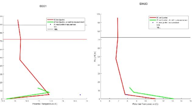
THERMAL INFLUENCES OVER THE SOUND:

The model’s incapability of correctly resolving stable sound cases could be a combination of upwind conditions and stable TIBL growth rates. An analysis of the information available about the evolution of the surface conditions over the sound for two cases (a stable and unstable case) is shown in Figure 22.

FIGURE 22:OSU1 CASE PROGRESSION

Figure 22 provides a spatial visualization of the upwind conditions in both a weakly unstable and strongly stable sound case. Vertical temperature measurements are shown from upwind of Pamlico Sound (red), above and within Pamlico Sound (green, where COARE results are associated), and at Billy Mitchell Airport (blue, where profiles were measured). In Figure 22a, the strongly stable sound case’s temperature profile is clearly stably stratified in the near-surface layer. However, the comparison of the RIBL height with the stable TIBL height indicate that the stable TIBL developing over Pamlico Sound is overwhelmed by the RIBL of Hatteras Island. The regions of low shear above the RIBL associated with the stable sound cases are most likely associated with the land surfaces upwind of Pamlico Sound, as opposed to the Pamlico Sound

FIGURE 23:PAMLICO SOUND SURFACE LAYER EVOLUTION

RIBL would be more representative of the unstable conditions, and therefore more adequately modeled with MOS.

T

The IBL height approximations were conducted using rough estimations of horizontal heterogeneity. The validity of these heights can be investigated by comparing them to the turbulence profiles provided by the SODAR. Knowledge of turbulence behavior is also necessary for wind energy engineering especially in areas of high variability - for both power curve estimations and evaluations of the material stresses of turbine blades. High levels of turbulence can cause unexpected effects (Honrubia, 2012). Especially in an unstable layer, turbulence measurements remain of interest despite the characteristically low levels of wind shear. The unstable regime is a convective region of the atmospheric boundary layer. While wind shear may remain low, turbulence can be unexpectedly high, especially if neutral stratification is assumed

FIGURE 24:OCEAN TURBULENCE PROFILES

based solely on wind profile measurements. It has been shown that the vertical distribution of turbulence can be characterized as a “traditional” boundary layer with upward transport of turbulent kinetic energy (TKE), or as an “upside-down” boundary layer, with downward transport of TKE (Mahrt & Vickers, 2002). The velocity variance profiles either decrease or increase with height, respectively, in these systems.

In the weakly stable ocean case (OWS3) presented in Figure 23, the vertical velocity variance seems to indicate that an “upside down” boundary layer begins at around the same height as the top of the TIBL. This finding may corroborate the TIBL method by suggesting a downward turbulent transport within the part of the wind profile associated with warmer, Gulf

FIGURE 25:SOUND TURBULENCE PROFILES

correspond to a maximum in backscatter intensity. The top of the RIBL could be a region of the wind profile with smaller scale turbulence as a result of mixing between the two distinct layers. Further, this result may suggest that a TIBL algorithm could be useful in wind energy development, in searching for regions far enough away from horizontal thermal gradients that high turbulence may be avoided. It is worth noting, however, that the “upside-down” boundary layer identified by Mahrt and Vickers is also characterized by a low-level wind maximum above the turbulence region. If wind turbine structures are able to withstand higher levels of turbulence structurally and maintain generation capabilities, the capacity payoff may be worthwhile.

In the sound cases, as seen in Figure 24, with SWU2, the RIBL seems to be significant to both the backscatter and the variance profiles. In the regions below the top of the RIBL, the variance and backscatter profiles are fairly uniform with height. This finding supports the RIBL algorithm by suggesting the roughness sub-layer is well-developed in the substantial overland fetch. The backscatter decreases slightly with height, typical of most of the sound cases regardless of stability regime. Although, some also exhibit the low-level maximum as seen in the ocean case discussed previously, possibly indicative of a second influential RIBL below the one calculated in the algorithm. The examples of decreasing velocity variance with height in the lower layers of the profile provide further evidence that the roughness elements of the island are indeed significant - a convergence of a “traditional” boundary layer (where roughness is the greatest factor) under an “upside-down” boundary layer (where the turbulent environment is more indicative of the water surface). The time periods where velocity variance increases with height within and above the RIBL suggest that the surface layer does not represent a “traditional” boundary layer. The wind speed profiles during these time periods agree with this implication – they display the most linearly shaped profiles, as opposed to the “traditional” logarithmically shaped profiles.

top of the TIBL. The variance measurements often increase greatly above this level. This shape is similar to the regions above the TIBL in the ocean cases, suggesting that an unstable TIBL for the sound might have existed at one point but is overcome by the significance of the RIBL over land. These turbulence measurements provide some confirmation that the IBL algorithms developed do provide reasonable estimates of the heights of significant change in the wind profile.

W

S

The RMS values determined from the deviation from the height-averaged mean in the wind profile provide a good indicator of the relative accuracy of the model in representing wind shear across an appropriate vertical range. The magnitude of wind shear throughout the profile is important to wind energy developers for its impacts on both total power available through the swept area of the turbine, as well as turbine loads and fatigue (Sathe, 2012), so confidence in MOST to provide an estimate of the wind shear is vital. The wind shear, related to the 𝑢_∗ value within the log-layer formulation, has been seen to vary with stability, most notably in the ocean cases. A comparison of the wind shear as approximated by the slope of the wind profile is shown in Figure 25, where a linear regression was performed through the applicable parts of the measured and modeled wind profiles for each case (surface to TIBL for stable ocean cases, and RIBL to top for sound cases and unstable ocean cases).

formulation also worked well for the near-neutral and stable sound cases. The average shear measured in sound cases (~0.02 s-1_{) was a roughly half of that in the ocean cases (~0.04 s}-1_).

Additionally, the measured shear in the sound cases was less varied (σ = 0.014 -1_{) than}

the measured shear in the ocean cases (σ = 0.033 s-1_{). In terms of predictability of wind shear}

across the swept area of a turbine, the stability-based model would improve the estimate within stable regimes, but would underestimate the value of the shear in neutral and unstable environments. However, in geographical areas or periods of time where shear is low, a characteristic of the sound cases, as in a land breeze or continental cold front combined with low fetches over water (<50km), the shear around turbine height could be well approximated with a constant value regardless of stability conditions.

FIGURE 26:SHEAR COMPARISON OF OCEAN CASES (A),SOUND CASES,(B)

S

M

E

The stability-based model in some cases offered improvements to estimations of both wind speed and wind shear. The degree to which the incorporated stability parameter improved the estimations depended on the upwind conditions, including directionality/marine surface, as well as stability regime. Wind speed estimation improvements are summarized across all cases in Table 2, by forming the difference of the modeled mean wind (height and temporal average) and the measured mean wind.

WIND SPEED (m/s) WIND SHEAR (1/s) *102

Model:

Cases:

Mean Measured

Neutral

Stability-based Mean

Measured

Neutral Stability-based

All 9.65 -1.50

-15.54%

-1.79

-18.55% 2.74

+1.96 +71.53%

+1.26 +45.99%

Sound 9.74 -1.12 -11.50%

-1.71

-17.56% 1.88

+1.24 +65.96%

+0.25 +13.30%

Ocean 9.52 -2.06 -21.64%

-1.91

-20.06% 4.02

+3.04 +75.62%

+2.76 +68.66%

Stable 9.06 -0.22 -2.43%

-3.15

-34.77% 3.51

+2.54 +72.36%

-0.63 -17.95%

Unstable 10.03 -1.60 -15.95%

-0.68

-6.78% 2.67

+1.97 +73.78%

+3.00 +112.36%

Stable

Sound 7.55

+0.85 +11.26%

-3.58

-47.42% 1.84

+1.43 +77.72%

-3.01 -163.59%

Unstable

Sound 10.86

-1.04 -9.58%

-0.03

-0.28% 1.86

+1.14 +40.27%

+1.49 +70.17%

Stable

Ocean 11.09

-1.64 -17.14%

-2.59

-27.01% 5.74

+4.03 +70.21%

+2.54 +44.25%

Unstable

Ocean 8.88

-2.38 -26.80%

-1.58

-17.79% 3.80

+3.13 +82.37%

+3.44 +90.53% TABLE 2:MEAN WIND SPEED AND WIND SHEAR DIFFERENCES

Wind shear is generally underestimated in both neutral and stability-based models. The scaled values, expressed as a percent improvement in the table, are largely affected by the stable sound outliers. When the stable sound cases SSS1 and SSS2 are removed from the average, the overall mean wind shear differences become +53.36% and +75.03% for the neutral and stability-based model respectively. These outliers indicate that the while the stability-based model may improve the estimation of shear in some cases if the TIBL growth rate is sufficient to clear any newly-developing IBLs, it can be greatly overestimated if this is not the case. Unstable cases are consistently worsened in a stability-based model regardless of marine surface. This is due to the expected decrease in shear with unstable atmospheric conditions not observed in the

FIGURE 27:OCEAN CASES WITH BUOY WIND SPEED

C

The results discussed above reveal that the MOST based COARE algorithm is useful in determining the wind profile structure in coastal environments, despite being developed for the open ocean. The shortcomings in estimating wind speed, wind shear, and in modeling the wind profile could be as much an effect of insufficient or unsuitable datasets as of inadequacies in the theoretical application. This is especially a concern in the complications present in analyzing winds coming from the sound, with varied and heterogeneous upwind conditions as well as significant roughness effects invading the wind profile. Mean wind speed estimations in unstable sound cases were improved using the stability-based model, but were the most poorly resolved in the stable cases. This is likely a result of the RIBL overwhelming a slowly-growing stable TIBL. Wind measurements in an onshore location with an overland fetch greater than 1 km would rarely retain evidence of a thermally stable marine surface layer within the wind profile.

backscatter measurements throughout the wind profile showed that knowledge of the environment’s stability characteristics provide information about IBLs and their relationship to turbulence that could be of use to wind farm development and operations.

W

C

Arya, S. Pal.

Introduction to Micrometeorology

. San Diego: Academic, 1988. Print.

Bane, John M., and William K. Dewar. "Gulf Stream Bimodality and Variability Downstream of

the Charleston Bump."

Journal of Geophysical Research

93.C6 (1988): 6695-710. Web.

Businger, J. A., J. C. Wyngaard, Y. Izumi, and E. F. Bradley. "Flux-Profile Relationships in the

Atmospheric Surface Layer."

Journal of the Atmospheric Sciences

28 (1971): 181-89.

Web.

Fairall, C. W., E. F. Bradley, J. E. Hare, A. A. Grachev, and J. B. Edson. "Bulk Parameterization

of Air-Sea Fluxes: Updates and Verification for the COARE Algorithm."

Journal of

Climate

16 (2003): 571-91. Web.

Foken, T, and C. J. Nappo.

Micrometeorology

. Berlin: Springer, 2008. Print.

Garratt, J.R., and B.F. Ryan. “The structure of the stably stratified internal boundary layer in

offshore flow over the sea.”

Boundary Layer Meteorology 47

(1989): 17-40.

Gualtieri, Giovanni, and Sauro Secci. "Methods to Extrapolate Wind Resource to the Turbine Hub

Height Based on Power Law: A 1-h Wind Speed vs. Weibull Distribution Extrapolation

Comparison."

Renewable Energy

43 (2012): 183-200. Web.

Holtslag, M. C., W. A.A.M. Bierbooms, and G.J. W. Van Bussel. "Validation of Surface Layer

Similarity Theory to Describe Far Offshore Marine Conditions in the Dutch North Sea in

Scope of Wind Energy Research."

Journal of Wind Engineering and Industrial

Aerodynamics

136 (2015): 180-191. Web.

Kaimal, J.C., and J.C. Wyngaard. “The Kansas and Minnesota Experiments.”

Boundary Layer

Meteorology.”

50 (1990): 31-37. Web.

Klaassen, Ger, Asami Miketa, Katarina Larsen, and Thomas Sundqvist. "The Impact of R&D on

Innovation for Wind Energy in Denmark, Germany and the United Kingdom."

Ecological

Economics

54 (2005): 227-40. Web.

Lange, Bernhard, Soren Larsen, Jorgen Hojstrup, and Rebecca Barthelmie. "The Influence of

Thermal Effects on the Wind Speed Profile of the Coastal Marine Boundary Layer."

Boundary Layer Meteorology

112 (2004): 587-617. Web.

Lantz, Eric, Ryan Wiser, and Maureen Hand.

IEA Wind Task 26: The Past and Future Cost of

Wind Energy

. Tech. no. 6A20-53510. Golden, CO: National Renewable Energy

Laboratory, 2012. Print.

Miller, Jerry L. "Fluctuations of Gulf Stream Frontal Position between Cape Hatteras and the

Straits of Florida."

Journal of Geophysical Research

99.C3 (1994): 5057-064. Web.

Obukhov, A. M. "'Turbulentnost' v Temperaturnoj - Neodnorodnog Atmosfere (Turbulence in an

Atmosphere with a Non-uniform Temperature)."

Geofiz AN SSSR

3 (1946): 95-115. Web.

Sathe, A., J. Mann, T. Barlas, W.A.A.M. Bierbooms, and G.J.W. van Bussel. “Influence of

atmospheric stability on wind turbine loads.”

Wind Energy

16 (2013): 1013-1032). Web.

Savidge, Dana K., Jay A. Austin, and Brian O. Blanton. "Variation in the Hatteras Front Density

and Velocity Structure Part 2: Historical Setting."

Continental Shelf Research

54 (2013):

106-16. Web.

Stull, Roland B.

An Introduction to Boundary Layer Meteorology

. Dordrecht: Kluwer Academic,

1988. Print.

Thomas, N., H. Seim, and S. Haines. "An Observational, Spatially Explicit, Stability-Based

Estimate of the Wind Resource off the Shore of North Carolina."

Journal of Applied

Meteorology and Climatology

54.12 (2015): 2407-425. Web.

UNC.

Coastal Wind: Energy for North Carolina's Future

. Rep. N.p.: UNC, 2009. Print.