Swarm and Evolutionary Computation 44 (2019) 945–956
Contents lists available atScienceDirect
Swarm and Evolutionary Computation
journal homepage:www.elsevier.com/locate/swevo
Multi-Objective Bayesian Global Optimization using expected hypervolume
improvement gradient
Kaifeng Yang
∗, Michael Emmerich, Andr
e Deutz, Thomas B
́
ack
̈
LIACS, Leiden University, Niels Bohrweg 1, 2333 CA, Leiden, the Netherlands
A R T I C L E I N F O
Keywords:
Bayesian global optimization Expected hypervolume improvement Expected hypervolume improvement gradient Kriging stopping criterion
A B S T R A C T
The Expected Hypervolume Improvement (EHVI) is a frequently used infill criterion in Multi-Objective Bayesian Global Optimization (MOBGO), due to its good ability to lead the exploration. Recently, the computational complexity of EHVI calculation is reduced toO(nlogn)for both 2-D and 3-D cases. However, the optimizer in MOBGO still requires a significant amount of time, because the calculation of EHVI is carried out in each iteration and usually tens of thousands of the EHVI calculations are required. This paper derives a formula for the Expected Hypervolume Improvement Gradient (EHVIG) and proposes an efficient algorithm to calculate EHVIG. The new criterion (EHVIG) is utilized by two different strategies to improve the efficiency of the optimizer discussed in this paper. Firstly, it enables gradient ascent methods to be used in MOBGO. Moreover, since the EHVIG of an optimal solution should be a zero vector, it can be regarded as a stopping criterion in global optimization, e.g., in Evolution Strategies. Empirical experiments are performed on seven benchmark problems. The experimental results show that the second proposed strategy, using EHVIG as a stopping criterion for local search, can outperform the normal MOBGO on problems where the optimal solutions are located in the interior of the search space. For the ZDT series test problems, EHVIG still can perform better when gradient projection is applied.
1. Introduction
Evolutionary Algorithms (EAs) and Bayesian Global Optimization (BGO) are two main branches in the field of optimization. Both of them share a similar structure: initialization, evaluation of a black box function at a given search point, an update of the current search point for seeking an improvement in the next loop and repetition of the evaluation and adjustment loop. The difference lies in the update mechanism. For EAs, this is accomplished by evolutionary operators, such as recombination and mutation. For the Bayesian global opti-mization, this is based on learning from the past evaluations and determining the next search point by optimization of an infill criterion formulated on that method. Compared to EAs, BGO requires only a small budget of function evaluations. Therefore, it can be applied to real-world optimization problems with expensive evaluations [1], e.g., evaluations occurring in computational fluid dynamics simulations or process control simulation.
In the context of Bayesian Global Optimization, a pre-selection or infill criterion is utilized to estimate the performance of the
∗Corresponding author.
E-mail addresses:[email protected](K. Yang),[email protected](M. Emmerich),[email protected](A. Deutz),t.h.w. [email protected](T. Bäck).
improvement for a new point. For single objective optimization,
Expected Improvement (EI) and Probability of Improvement (PoI) are
usually applied in BGO. The EI was introduced by Mockus et al. [2] in 1978, and it exploits both the Kriging prediction and the variance to give a quantitative measure of the improvement for the points in the search space. Later, EI became more popular due to the work of Jones et al. [3]. Currently, EI is widely used in Bayesian Global Optimization and machine learning. In 2005, Emmerich generalized EI into EHVI based on the hypervolume indi-cator [4]. Similar to EI, the EHVI is the expected increment of the hypervolume indicator, considering a Pareto-front approximation set and a predictive multivariate Gaussian distribution at a new point.
EHVI has been in existence for more than a decade, and it has the property to achieve a good convergence and diversity to a true Pareto front [5–8]. It also yields good results when applied as an infill criterion in BGO and pre-selection criterion in Evolution Strategies in optimiza-tion studies. However, it was frequently criticized for the high computa-tional effort that seemed to be required when computing the underlying
https://doi.org/10.1016/j.swevo.2018.10.007
Received 27 September 2017; Received in revised form 24 September 2018; Accepted 15 October 2018 Available online 28 October 2018
multi-variable integrals. The first method suggested for EHVI calcula-tion was Monte Carlo integracalcula-tion and it was first proposed by Emmerich in Refs. [4] and [9]. This method is simple and straightforward. How-ever, the accuracy of EHVI highly depends on the number of the iter-ations. The first exact EHVI calculation algorithm for a 2-D case was derived in Ref. [10], with the computational complexityO(n3 logn).
Couckuyt et al. introduced exact EHVI calculation ford>2 in Ref. [5]. This method was also practically much faster than those discussed in Ref. [10], although a detailed complexity analysis was missing. In 2015, Hupkens et al. reduced the time complexity toO(n2)andO(n3) [11]
for the two and the three-dimensional case, respectively. These algo-rithms also further improved the practical efficiency of EHVI on test data. However, there still exists a large gap to use EHVI in applica-tions. Considering the expensive computation of EHVI and inspired by the EHVI, Couckuyt et al. proposed theHypervolume based Probability of
Improvementin Ref. [5]. Luo et al. used an approximate algorithm to
cal-culate EHVI based on Monte Carlo sampling for high dimensional cases (d>6) in Ref. [7], wheredstands for the dimension in objective space. Finally, Emmerich et al. proposed an asymptotically optimal algorithm for the bi-objective case with time complexityΘ(nlogn)in Ref. [12], wherenis the number of non-dominated points in the archive. More recently, Yang et al. [13] proposed an algorithm to calculate 3-D EHVI with computational complexityΘ(nlogn).
However, compared to EAs, Multi-Objective Bayesian Global Opti-mization still performs much slower with the infill criterion EHVI, because EHVI needs to be called many times in the process of searching for the optimal point based on the Kriging models. Since the calcula-tion of the EHVI can be formulated in closed form, it is possible to analyze its differentiability. It is easy to see, that all components of the EHVI expression are differentiable. However, a precise formula of the EHVIG has not been derived until now. By using the formula for the EHVIG, it could speed up the MOBGO in the process of searching for the optimal point by using the gradient ascent algorithm or using it as a stopping criterion in EAs. This is the motivation of the research in this paper.
This paper mainly discusses the computation of the 2-D EHVIG and how to apply EHVIG in MOBGO, both for local search (gradient ascent) and as a stopping criterion. The paper is structured as fol-lows: Section 2briefly describes Bayesian Global Optimization, some basic infill criteria, and how to compute 2-D EHVI efficiently; Section 3introduces the definition of the EHVIG, and proposes an efficient algorithm to calculate 2-D EHVIG, including a computational perfor-mance assessment of the proposed efficient exact calculation method and numerical calculation method in 2-D EHVIG case; Section4 intro-duces the techniques on how to apply EHVIG in MOBGO; Section5 shows some empirical, experimental results; Section6draws the main conclusions of this paper and discusses some potential topics for future research.
2. State of the art1
2.1. Bayesian Global Optimization
Bayesian Global Optimization(BGO), also known asEfficient Global
Optimization [3] or Expected Improvement Algorithm [14], was
pro-posed by the Lithuanian research group of Jonas Mockus and Antanas ̌Zilinskas ([2,15–17]) in the 1970s. In BGO, it is assumed that the objec-tive function is the realization of a Gaussian random field, which is also called Gaussian process (GP) or Kriging, in particular in 1-D.
Kriging is a statistical interpolation method. Being a Gaussian pro-cess based modelling method, it is cheap to evaluate [18]. Kriging has been proven to be a popular surrogate model to approximate
1For the convenience of the visualization, this paper only considers
mini-mization problems.
noise-free data in computer experiments, where Kriging models are fitted on previously evaluated points and then replace the real time-consuming simulation model [19]. Given a set ofndecision vectorsX= (x(1),x(2), · · ·,x(n))⊤ in m dimensional search space, and associated
function valuesy(X) = (y(x(1)),y(x(2)),…,y(x(n)))⊤, Kriging assumesy to be a realization of a random processYand it is of the form [3,20]:
Y(x) =𝜇(x) +𝜖(x) (2-1)
where𝜇(x)is estimated mean value over all given sampled points, and 𝜖(x)is a realization of a normally distributed Gaussian random process with zero mean and variance𝜎2. The regression part𝜇(x)approximates
globally the functionYand Kriging/Gaussian process𝜖(x)takes local variations into account. Moreover, as opposed to other regression meth-ods, such as supported vector machine (SVM), Kriging/GP also provides an uncertainty qualification of a prediction. The correlation between the deviations at two points (xandx′) is defined as:
Corr[𝜖(x), 𝜖(x′)] =R(x,x′) =
m ∏
i=1
Ri(xi,x′i) (2-2)
HereR(., .)is the correlation function, which can be a cubic or a spline function. Commonly, a Gaussian function (also known as squared expo-nential) is chosen:
R(x,x′) =
m ∏
i=1
exp(−𝜃i(xi−x′i)
2) (𝜃
i>=0) (2-3)
where𝜃 are parameters of correlation model and they can be inter-preted as measuring the importance of the variable. Then the covari-ance matrix can be expressed by the correlation function:
Cov(𝝐) =𝜎2𝚺, where 𝚺i
,j=R(xi,xj) (2-4)
When𝜇(x)is assumed to be an unknown constant, this unbiased pre-diction is called ordinary Kriging (OK). In OK, the Kriging model deter-mines the hyperparameters𝜽= [𝜃1, 𝜃2,…, 𝜃n]by maximizing the likeli-hood of the observed dataset. The expression of the likelilikeli-hood function is:
L= −n
2ln(𝜎
2) −1
2ln(|𝚺|) (2-5)
The maximum likelihood estimates of the mean𝜇̂and the variancê𝜎2
are given by Ref. [3]:
̂ 𝜇= 1
⊤ n𝚺
−1y
1⊤n𝚺−11n (2-6)
̂𝜎2=1
n(y−1n𝜇̂)
⊤𝚺−1(y−1
n𝜇̂) (2-7)
Then the predictor of the mean and the variance at point xtcan be
derived and they are shown as follows [3]: 𝜇(xt) =𝜇̂+c⊤𝚺−1(y−𝜇̂1
n) (2-8)
𝜎2(xt) =̂𝜎2
(
1−c⊤𝚺−1c+1−c⊤Σ⊤c 1⊤nΣ−11n
)
(2-9)
wherec= (Corr[Y(xt),Y(x
1)],…,Corr[Y(xt),Y(xn)])⊤. The time com-plexity of computing these values at an input vector x, once the hyperparameters are fixed, is (O(mn))per computation of 𝜇̂(.), and O(n2+mn)per computation of̂𝜎(.).
The basic idea of BGO is to use a surrogate model based on Krig-ing or a Gaussian process. A surrogate model reflects the relation-ship between decision vectors and their corresponding objective val-ues. This surrogate model is learned from previous evaluations. For multi-objective problems, the family of these algorithms is called
Multi-Objective Bayesian Global Optimization (MOBGO). The scheme of a
K. Yang et al. Swarm and Evolutionary Computation 44 (2019) 945–956
2.2. Infill criteria
InMulti-Objective Bayesian Global Optimization, some commoninfill
criteriaare:Hypervolume Indicator(HV) [21],Hypervolume Improvement
(HVI) [22],2 Hypervolume Contribution(HVC) [23], Lower Confidence
Bound(LCB) [9,24,25], EHVI [4,26],Probability of Improvement (PoI)
[27] andTruncated Expected Hypervolume Improvement(TEHVI) [28,29]. Many of these are based on the hypervolume indicator.
The HV was proposed by Zitzler and Thiele [30], and it measures the size of the dominated subspace bounded from above by a refer-ence pointr. This reference point should be chosen by a user, and it should satisfy the condition that it is dominated by all the elements of the Pareto-front approximation sets which might occur during the opti-mization process, if possible. The hypervolume can indicate the perfor-mance of a Pareto-front approximation set⊂ℝd, and the maximiza-tion of HV can lead to a Pareto-front approximamaximiza-tion set that is close to the true Pareto front. In 2-D and 3-D cases, the hypervolume indicator can be computed in timeΘ(nlogn)[31]. In more than 3 dimensions,
the algorithm proposed by Chan [32] achievesO (
nd3polylogn )
time
complexity. The hypervolume indicator is defined as:
Definition 2.1. (Hypervolume Indicator)Given a finite approximation
to a Pareto front, say= {y(1),…,y(n)}⊂ℝd,the Hypervolume Indicator
(HV) ofis defined as the d -dimensional Lebesgue measure of the subspace
dominated byand bounded from above by a reference pointr:
HV() =𝜆d(∪y∈[y,r]) (2-10)
with𝜆dbeing the Lebesgue measure onℝd.
Two straightforward derived criteria are the HVI and the HVC. Emmerich et al. proposed an asymptotically optimal algorithm to calcu-late HVC with time complexityΘ(nlogn)ford=2,3 in Ref. [33]. The basic idea behind these two criteria is the same, that is to calculate the difference of the hypervolume between two Pareto-front approximation sets. The definition of HVC of a pointy∈is the difference between the hypervolume of and the hypervolume of⧵{y}.Hypervolume
Improvementis defined as:
Definition 2.2. (Hypervolume Improvement)Given a finite collection
of vectors⊂ℝd, the Hypervolume Improvement of a vectory∈ℝdis
defined as:
HVI(,y) =HV(∪ {y}) −HV() (2-11)
In case we want to emphasize the reference pointr,the notationHVI(,y,r)
will be used to denote the Hypervolume Improvement. Note thatHVI(,y) =
0,in casey∈.
EHVI is a generalization of EI to the multi-objective case, based on the theory of the HV. Similar to EI, the definition of EHVI is with respect to the predictions in the Gaussian random field and it measures how much hypervolume improvement could be achieved by evaluating the new point, considering the uncertainty of the prediction. It is defined as:
Definition 2.3. (Expected Hypervolume Improvement)3 Given
parameters of the multivariate predictive distribution𝝁,𝝈and the
Pareto-front approximation the expected hypervolume improvement (EHVI) is
defined as:
EHVI(𝝁,𝝈,,r)≔ ∫
ℝd
HVI(,y) ·PDF𝝁,𝝈(y)dy (2.12)
where PDF𝝁,𝝈is the multivariate independent normal distribution for mean
values𝝁∈ℝd,and standard deviations𝝈∈ℝd
+.
2The HVI was called the most likely improvement (MLI) in Ref. [22]. 3The prediction of𝛍and𝛔depends on a Kriging model and a target pointx
in the search space. Explicitly, EHVI is dependent on the target pointx.
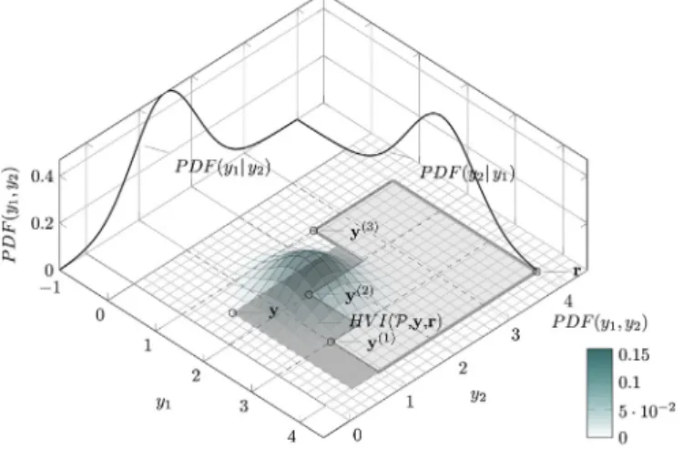
Fig. 1.EHVI in 2-D (cf.Example 2.1).
Example 2.1. An illustration of the EHVI is shown inFig. 1. The light gray area is the dominated subspace of= {y(1)= (3,1)⊤, y(2)=
(2,1.5)⊤, y(3)= (1,2.5)⊤} cut by the reference point r= (4,4)⊤. The
bivariate Gaussian distribution has the parameters 𝜇1=2, 𝜇2=1.5,
𝜎1=0.7, 𝜎2=0.6.The probability density function (PDF) of the
bivari-ate Gaussian distribution is indicbivari-ated as a 3-D plot. Hereyis a sample from
this distribution and the area of improvement relative to is indicated by
the dark shaded area. The variable y1stands for the f1value and y2for the
f2value.
For the convenience of expressing the formula of EHVI and EHVIG in later sections, it is useful to define a function we callΨ.
Definition 2.4. (Ψ function (see also [11])) Let 𝜙(s) =
1∕√2𝜋e−12s2,s∈ℝdenote the PDF of the standard normal distribution and
Φ(s) =12 (
1+erf (
s √
2
))
denote its cumulative probability distribution
function (CDF). The general normal distribution with mean𝜇and variance
𝜎 has the PDF 𝜙𝜇,𝜎(s) =1𝜎𝜙(s−𝜎𝜇) and the CDF 𝛷𝜇,𝜎(s) = Φ(s−𝜎𝜇).
Moreover, a useful identity which we will frequently use is:
b
∫ −∞
(a−z)1
𝜎𝜙(z−𝜎𝜇)dz=𝜎𝜙(b−𝜎𝜇) + (a−𝜇)Φ (
b−𝜇
𝜎 )
(2-13)
.We define the functionΨas follows:
Ψ(a,b, 𝜇, 𝜎)≔
b
∫ −∞
(a−z)1𝜎 𝜙(z−𝜎𝜇)dz (2-14)
2.3. Efficient algorithm for 2-D EHVI calculation
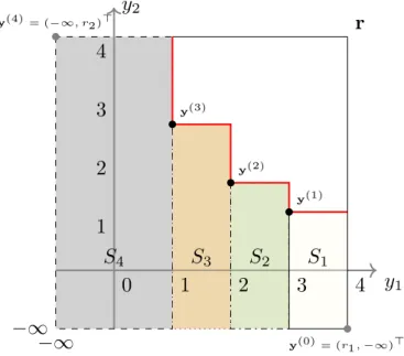
This paper focuses on bi-objective problems. The calculation of EHVIG in Section3shares the same partitioning method with 2-D EHVI calculation and EHVIG is derived from EHVI. Therefore, it is neces-sary to introduce an efficient algorithm for 2-D EHVI calculation, as described in the recent work by Emmerich et al. [12].
The partitioning of the integration domain is done by the fol-lowing steps: augment the current Pareto-front approximation = {y(1),…,y(n)} by two more points y(0)= (r
1,−∞)⊤ and y(n+1)=
(−∞,r2)⊤; sort the points inin ascending order by the second
coordi-nate of the points. Then, the domicoordi-nated space will be divided inton+1 disjoint rectangular stripesS1,…,Sn+1, and these stripes are defined by:
Si=
(
(y(1i),−∞)⊤,(y1(i−1),y(2i))⊤)i=1,…,n+1 (2-15)
Fig. 2.Partitioning of the integration region into stripes.
For the convenience of computing EHVI, it is useful to define the functionΔ, which is defined as:
Definition 2.5. (Δfunction(see also[12]))For a given vector of
objec-tive function values,y∈ℝd, Δ(y,,r) is the subset of the vectors inℝd
which are exclusively dominated by a vectoryand not by elements inand
that dominate the reference point, in symbols
Δ(,y,r) =𝜆d{z∈ℝ|y≺zandz≺rand∄q∈∶q≺z} (2-16)
For the simplicity, the notation Δ(y) will be used to express Δ(,y,r)in this paper.
Then, the hypervolume improvement of a point y∈ℝ2 can be
expressed by:
HVI(,y,r) = n+1
∑
i=1
𝜆2[Si∩ Δ(y1,y2)] (2-17)
Here,Δ(y1,y2)is the part of the objective space that is dominated
byy= (y1,y2). Recall the definition of EHVI, then the EHVI formula
can be derived that consists ofn+1 integrals:
EHVI(𝝁,𝝈,,r) =
∞
∫
y1=−∞ ∞
∫
y2=−∞
n∑+1
i=1
𝜆2[Si∩ Δ((y1,y2))]
·PDF𝝁,𝝈(y1,y2)dy1dy2 (2-18)
It is observed that the intersection ofSiwithΔ(y1,y2)is non-empty
if and only ify= (y1,y2)dominates the upper right corner ofSi, and it
is allowed to do the summation after integration since integration is a linear mapping, therefore:
EHVI(𝝁,𝝈,,r) = n+1
∑
i=1
y1(i−1)
∫
y1=−∞ y(2i)
∫
y2=−∞
𝜆2[Si∩ Δ(y1,y2)]
·PDF𝝁,𝝈(y1,y2)dy1dy2 (2-19)
After some basic derivations, the final expression for the 2-D EHVI is [12]
EHVI(𝝁,𝝈,,r) = n∑+1
i=1
(y(1i−1)−y(1i)) · Φ (
y(1i)−𝜇1
𝜎1
)
· Ψ(y(2i),y2(i), 𝜇2, 𝜎2)
+ n∑+1
i=1
(
Ψ(y1(i−1),y1(i−1), 𝜇1, 𝜎1) − Ψ(y1(i−1),y
(i)
1, 𝜇1, 𝜎1)
)
· Ψ(y2(i),y2(i), 𝜇2, 𝜎2) (2-20)
3. Expected hypervolume improvement gradient
This section will mainly introduce the definition of EHVIG, how to calculate EHVIG and show some performance assessment between the exact calculation method and the numerical calculation method.
3.1. Definition
Considering the definition of the EHVI in Equation(2.5)and the effi-cient algorithm to calculate 2-D EHVI (minimization case), the EHVI is differentiable with respect to the predictive mean and its correspond-ing standard deviation provided, which is greater than zero. These two parameters, predictive mean and standard deviation, are again differ-entiable with respect to the input vector (or target point) in the search space. The EHVIG is the first order derivative of the EHVI with respect to a target pointxunder consideration in the search space. It is defined as:
Definition 3.1. (Expected Hypervolume Improvement Gradient)4
Given parameters of the multivariate predictive distribution𝝁,𝝈at a target
pointxin the search space, the Pareto-front approximation,and a
refer-ence pointr,the expected hypervolume improvement gradient (EHVIG) atx
is defined as:
EHVIG(x,𝝁,𝝈,,r) =𝜕(EHVI(𝝁,𝝈,,r))
𝜕x
=𝜕 (
∫ℝdHVI(,y) ·PDF𝝁,𝝈(y)dy )
𝜕x (3-1)
3.2. Formula derivation
According to the definition of EHVIG in Equation(3-1)and the effi-cient algorithm to calculate EHVI in Equation(2-20), we can substitute the Equation(2-20)into Equation(3-1), say that the formula of EHVIG for 2-D case can be expressed as:
EHVIG(x,𝝁,𝝈,,r) =𝜕(EHVI(𝝁,𝝈,,r))
𝜕x
= 𝜕(∑n+1
i=1(y
(i−1)
1 −y
(i)
1) · Φ(
y(1i)−𝜇1 𝜎1 ) · Ψ(y
(i)
2,y
(i)
2, 𝜇2, 𝜎2)
)
𝜕x (3-2)
+𝜕 (∑n+1
i=1
(
Ψ(y(1i−1),y1(i−1), 𝜇1, 𝜎1) − Ψ(y(1i−1),y
(i)
1, 𝜇1, 𝜎1)
)
· Ψ(y(2i),y2(i), 𝜇2, 𝜎2)
)
𝜕x (3-3)
For the Terms(3-2)and(3-3), the prerequisite of calculating these two Terms is to calculate the gradient of theΨfunction and of the
Φ(y−𝜎𝜇)function. The final expressions for 𝜕Ψ(a𝜕,bx,𝜇,𝜎) and 𝜕Φ(
y−𝜇 𝜎 )
𝜕x are
4The prediction of𝛍and𝛔depends on a Kriging model and a target pointx
K. Yang et al. Swarm and Evolutionary Computation 44 (2019) 945–956
shown in Equation(3-4)and Equation(3-5), respectively. For detailed proofs, please refer to theAppendixof this paper.
𝜕Ψ(a,b, 𝜇, 𝜎)
𝜕x =
(
b−a
𝜎 ·𝜙(b−𝜎𝜇) − Φ(b−𝜎𝜇) )
·𝜕𝜇 𝜕x
+𝜙(b−𝜇 𝜎 ) ·
(
1+(b−𝜇)(b−a) 𝜎2
) ·𝜕𝜎
𝜕x (3-4)
𝜕Φ(y−𝜎𝜇) 𝜕x =𝜙(
y−𝜇
𝜎 ) · (𝜇𝜎−2y·𝜕𝜎𝜕x−
1
𝜎·𝜕𝜇𝜕x) (3-5)
By substituting Equations(3-4) and (3-5)into Term(3-2)and apply-ing the chain rule, Term(3-2)can be expressed by:
𝜕(∑n+1
i=1(y
(i−1)
1 −y
(i)
1) · Φ(
y(1i)−𝜇1 𝜎1 ) · Ψ(y
(i)
2,y
(i)
2, 𝜇2, 𝜎2)
)
𝜕x
= n+1
∑
i=1
(y(1i−1)−y1(i)) · 𝜕(Φ(y
(i) 1−𝜇1
𝜎1 ) · Ψ(y
(i)
2,y
(i)
2, 𝜇2, 𝜎2)
)
𝜕x
= n+1
∑
i=1
(y(1i−1)−y1(i)) · (
𝜙(y
(i)
1 −𝜇1
𝜎1
) · (𝜇1−y
(i)
1
𝜎2 1
·𝜕𝜎1
𝜕x − 1 𝜎1
·𝜕𝜇1
𝜕x) · Ψ(y (i)
2,y
(i)
2, 𝜇2, 𝜎2) +
( 0− Φ((y
(i)
2 −𝜇2)
𝜎2
·𝜕𝜇2
𝜕x)
+𝜙(y
(i)
2 −𝜇2
𝜎2
) · (1+0) ·𝜕𝜎2 𝜕x )
· Φ(y
(i)
1 −𝜇1
𝜎1
) )
= n+1
∑
i=1
(y(1i−1)−y1(i)) · (
𝜙(y
(i)
1 −𝜇1
𝜎1
) · (𝜇1−y
(i)
1
𝜎2 1
·𝜕𝜎1
𝜕x
− 1 𝜎1
·𝜕𝜇1
𝜕x) · Ψ(y (i)
2,y
(i)
2, 𝜇2, 𝜎2) +
( 𝜙(y
(i)
2 −𝜇2
𝜎2
) ·𝜕𝜎2
𝜕x
− Φ(y
(i)
2 −𝜇2
𝜎2
) ·𝜕𝜇2
𝜕x )
· Φ(y
(i)
1 −𝜇1
𝜎1
) )
(3-6)
Similar to the derivation of Term(3-2), Term(3-3)can be expressed by:
𝜕(∑n+1
i=1
(
Ψ(y(1i−1),y1(i−1), 𝜇1, 𝜎1) − Ψ(y(1i−1),y
(i)
1, 𝜇1, 𝜎1)
)
· Ψ(y(2i),y2(i), 𝜇2, 𝜎2)
)
𝜕x
= n+1
∑
i=1
⎛ ⎜ ⎜ ⎝
𝜕(Ψ(y(1i−1),y1(i−1), 𝜇1, 𝜎1) − Ψ(y1(i−1),y
(i)
1, 𝜇1, 𝜎1)
)
𝜕x · Ψ(y
(i)
2,y
(i)
2, 𝜇2, 𝜎2)
+𝜕Ψ(y
(i)
2,y
(i)
2, 𝜇2, 𝜎2)
𝜕x ·
(
Ψ(y(1i−1),y1(i−1), 𝜇1, 𝜎1) − Ψ(y(1i−1),y
(i)
1, 𝜇1, 𝜎1)
))
= n+1
∑
i=1
⎛ ⎜ ⎜ ⎝
𝜕(Ψ(y(1i−1),y(1i−1), 𝜇1, 𝜎1)
)
𝜕x · Ψ(y
(i)
2,y
(i)
2, 𝜇2, 𝜎2)
−𝜕 (
Ψ(y(1i−1),y(1i), 𝜇1, 𝜎1)
)
𝜕x · Ψ(y
(i)
2,y
(i)
2, 𝜇2, 𝜎2) +
𝜕Ψ(y(2i),y2(i), 𝜇2, 𝜎2)
𝜕x ·(Ψ(y(1i−1),y1(i−1), 𝜇1, 𝜎1) − Ψ(y(1i−1),y(1i), 𝜇1, 𝜎1)
))
= n+1
∑
i=1
(( 𝜙(y
(i−1)
1 −𝜇1
𝜎1
) ·𝜕𝜎1
𝜕x − Φ(
y(1i−1)−𝜇1
𝜎1
) ·𝜕𝜇1
𝜕x )
· Ψ(y2(i),y2(i), 𝜇2, 𝜎2) −
( [y
(i)
1 −y
(i−1)
1
𝜎1
·𝜙(y
(i)
1 −𝜇1
𝜎1
) − Φ(y
(i)
1 −𝜇1
𝜎1
)]
·𝜕𝜇1
𝜕x + [𝜙( y(1i)−𝜇1
𝜎1
) · (1+(y
(i)
1 −𝜇1)(y
(i)
1 −y
(i−1)
1 )
𝜎2 1
)] ·𝜕𝜎1
𝜕x )
· Ψ(y2(i),y2(i), 𝜇2, 𝜎2) +
( 𝜙(y
(i)
2 −𝜇2
𝜎2
) ·𝜕𝜎2
𝜕x − Φ( y(2i)−𝜇2
𝜎2
) ·𝜕𝜇2
𝜕x )
·
×(Ψ(y1(i−1),y1(i−1), 𝜇1, 𝜎1) − Ψ(y1(i−1),y
(i)
1, 𝜇1, 𝜎1)
))
(3-7)
Then, the EHVIG is the sum of Terms(3-6)and(3-7). In these two Terms,𝜕𝜇i𝜕x and𝜕𝜎i𝜕x (i=1,2) are the first order derivatives of the Kriging predictive means and standard deviations at a target pointx, respec-tively. These parameters can be precisely calculated by the following equations [34,35]:
𝜕𝜇 𝜕x=
𝜕c⊤ 𝜕x𝚺
−1
( y− 1
⊤ nΣ−1y 1⊤nΣ−11
n 1n
)
(3-8)
𝜕𝜎 𝜕x= −
1 𝜎𝜕c
⊤ 𝜕x𝚺
−1
( c−1−1
⊤ nΣ
−1c
1⊤nΣ−11n 1n
)
(3-9)
where𝜕c
𝜕x=2 diag(𝜃1,…, 𝜃n) · [R(x,x1)(x1,x),…,R(x,xn)(xn,x)] (3-10)
Compared to the final expression of 2-D EHVI in Equation(2-20), the final expression of 2-D EHVIG also consists of two terms, Term (3-6)and Term(3-7). Moreover, the number of the integration stripes both in EHVIG and EHVI isn+1, as we are using the EHVI partition-ing method in EHVIG. Therefore, the computational complexity of 2-D EHVIG is equal to the complexity of EHVI, that isO(nlogn). For the detailed proof of 2-D EHVI computational complexity, see Ref. [12]. Note, that thisO(nlogn)complexity does not include the time required for computing𝝁and𝝈, which was discussed earlier and depends on the surrogate modelling approach.
3.3. Performance assessment
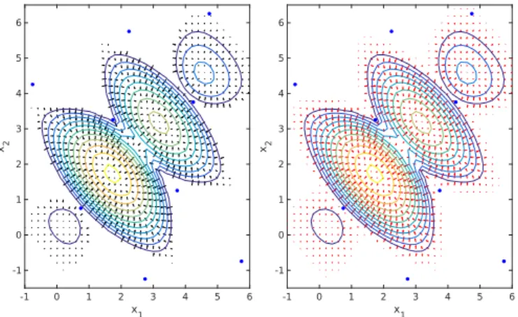
The performance assessment of the EHVIG will be illustrated by a single numerical experiment. The bi-criteria optimization problem is:
y1(x) = ∥x−1∥→min,y2(x) =‖x+1‖→min, x∈ [−1,6] × [−1,6]⊂
ℝ2 [12]. Fig. 3shows the landscape of EHVIG, in which the
evalu-ated points are marked by blue circles. The EHVIG calculevalu-ated by the exact method,5which uses EHVIG formula in section3.2, is indicated by black arrows in the left figure. The EHVIG calculated by the numeri-cal method, which meshgrids a search space and numeri-calculate the difference
5The MATLAB source code for computing the EHVIG for 2-D case is available
Fig. 3.The landscape of EHVIG. Left: computed using exact calculation algo-rithm, Right: computed using numerical calculation method.
of the EHVI values between numerical differential two points, is indi-cated by the red arrows in the right figure. The landscapes of EHVIG in both figures are very similar, however, there exist some slight differ-ences between them, while very small and caused by numerical errors.
4. Multi-Objective Bayesian Global Optimization based on EHVIG
Similar to BGO, Multi-Objective Bayesian Global Optimization (MOBGO) is also based on Kriging theory. MOBGO assumes that d objective functions are mutually independent in an objective space. In MOBGO, the Kriging method or Gaussian process can approximate the objective functions and quantify the uncertainties of the prediction by using Kriging models, which are determined by the existing evaluation dataD=((x(1),y(1)=Y(x(1))),…,(x(𝜇),y(𝜇)=Y(x(𝜇)))). Each objective function at a given pointx(t)is approximated by a one-dimensional
nor-mal distribution, with mean𝜇and standard deviation𝜎. Then MOBGO can predict the multivariate outputs by means of an independent joint normal distribution with parameters𝜇1,…,𝜇dand𝜎1,…,𝜎dat the pointx(t).
These predictive means and standard deviations can be used to cal-culate infill criteria. Aninfill criterionmeasures how promising a new point is when compared to a current Pareto-front approximation. With the assistance of a single objective optimization algorithm, the ‘optimal’ solutionx∗can be found according to the score of the infill criterion. This score of the infill criterion is calculated by the predictions of the Kriging models, instead of by the direct evaluations of the objective functions. Subsequently, the algorithm evaluates the ‘optimal’ solution x∗, and both the datasetDand the Pareto-front approximation setare updated.
The basic structure of the MOBGO algorithm is shown in Algo-rithm 1. Note that only one criterionCis chosen in a certain MOBGO, and this criterion defines the variations of MOBGO inAlgorithm 1line 8. Some common infill criteria are:Probability of Improvement (PoI), EHVI andHypervolume Improvement(HVI)·In this paper, the infill crite-rion is EHVI. Here,optis a search algorithm which finds the optimal solutionx∗by maximizing the EHVI.
4.1. Gradient ascent algorithms
Previously, the optimizeroptinAlgorithm 1was chosen as CMA-ES [36], which is a state-of-the-art heuristic global optimization algorithm. Since the formula of 2-D EHVIG is derived in this paper, a gradient ascent algorithm can replace CMA-ES to speed up the process of finding a promising pointx∗.
Many gradient ascent algorithms (GAAs) exist. The conjugate gra-dient algorithm is one of the most efficient algorithms among them. However, it cannot solve the constrained problems, and this is the
rea-son why we exclude it in this paper. For the other GAAs, the general formula for computing the next solution is:
x(t+1)=x(t)+s· ∇F(x(t)) (4-1)
wherex(t)is the current solution,x(t+1)is the updated solution,sis the
stepsize, and∇F(·)is the gradient of the objective functions or of the infill criterion. In this paper,∇Fis EHVIG.
Another important aspect is that the starting point is crucial to the performance of GAAs. To improve the probability of finding the globally optimal location, CMA-ES was used to initialize the starting points in this paper. The structure of gradient ascent based search algorithm is shown inAlgorithm 2.
4.2. EHVIG as a stopping criterion for CMA-ES
Traditionally, when EAs are searching for the promising pointx∗, convergence velocity and some other statistical criteria are used to determine whether the EAs should stop/restart or not. These criteria can balance the quality of the performance and efficiency of the execu-tion time to some degree, but not optimally. Because all these criteria are blind to whether an individual is already the optimal or not.
Considering that the gradient of the promising point in the search space should be the zero vector and EHVIG can be exactly calculated, EHVIG can be used as a stopping/restart criterion in EAs when they are searching for the optimal point with the EHVI as the infill criterion. Theoretically speaking, the EHVI should be maximized during the pro-cedure. Therefore, for this method it is necessary to use, for instance, information about the second derivative of the EHVI at this point, in order to determine the optimality and the type of optimality. However, this is omitted due to the complexities. The structure of CMA-ES assisted by EHVIG is shown inAlgorithm 3.
5. Empirical experiments
The benchmarks were well-known test problems: BK1 [37], SSFYY1 [38], ZDT1, ZDT2, ZDT3 [39], the generalized Schaffer problem [40] with different parameter settings for𝛾(𝛾in GSP and GSP12 were 0.4 and 1.2, respectively), and three proportional-integral-derivative (PID) parameter tuning problems [41–43].
5.1. Test problem 1 - Robust PID parameter tuning
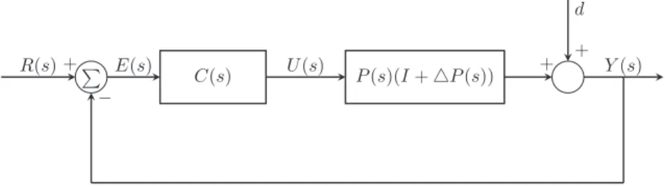
A PID controller is a control loop feedback mechanism, and it is widely applied in industrial control applications. The structure of the feedback controller is shown inFig. 4, whereR(s)is the reference input signal,E(s)represents error signal,C(s)is the transfer function of the controller,U(s)is control signal,P(s)stands for controlled plant,△P(s) is the plant perturbation,d(t) is the external disturbance andY(s)is the output of the system. For the PID controller, three parameters are part ofC(s): proportionalityB2, integralB1 and derivativeB0, and the transfer function of the PID controller for a continuous system can be defined as:C(s) = B2s2+B1ss +B0. The basic idea of a PID controller is to attempt to minimize an error (E(s)) by adjusting the process control inputs.
The benchmark for PID parameter tuning is taken from Ref. [41,44]. The transfer function of the plant is given as follows:
P(S) =
⎛ ⎜ ⎜ ⎜ ⎝
−33.98 (98.02s+1)(0.42s+1)
32.63 (99.6s+1)(0.35s+1) −18.85
(75.43s+1)(0.30s+1)
34.84 (110.5s+1)(0.03s+1)
⎞ ⎟ ⎟ ⎟ ⎠
(5-1)
Two criteria were used in this paper: balanced performance criterion
J∞= (J2a+J2b)
1∕2 [45] and interval squared errorJ
2=∫0∞e⊤(t)e(t)dt.
K. Yang et al. Swarm and Evolutionary Computation 44 (2019) 945–956
Algorithm 1 MOBGO algorithm.
Algorithm 2 Gradient ascent based search algorithm.
‖W2(s)S(s)‖∞. Here,W1(s) is the assumed boundary of plant
pertur-bation△P(s),W2(s)is a stable weighting function matrix and they are defined in Ref. [45]:
W1(s) = s100+1000s+1×I2×2, (5-2)
W2(s) = 1000s+1000s+1×I2×2. (5-3)
T(s)andS(s)are the sensitivity and complementary sensitivity functions of the system, respectively, and they can be calculated by:
S(s) = (I+P(s)C(s))−1, (5-4)
T(s) =P(s)C(s)(I+P(s)C(s))−1. (5-5)
5.2. Test problem 2 - PID parameter tuning problem
This benchmark on PID parameter tuning is taken from Ref. [43]. The three parameters for the PID controller are: proportionalityKp, inte-gralKiand derivativeKd. The transfer function of PID controller for a continuous system can be defined as:Y(s) = UE((ss))=Kp+Ksi+Kds. The process of PID controller can be described as follows: when a setpoint is set orE(s)exists,E(s)will be calculated by the difference between the setpoint and actual output, and a PID controller will generate a new control signal (U(s)) based onE(s). Then the new control signalU(s) is applied to the plant model, and the new actual output andE(s)are generated again. The structure of a PID control is shown inFig. 5.
The chosen transfer functions modelling the plant in this paper are:
G1(s) = 25.2s
2+21.2s+3
s5+16.58s4+25.41s3+17.18s2+11.70s+1[42] (5-6)
Fig. 4.Feedback control system with plant perturbation and external disturbance.
Fig. 5.The structure of PID control.
G2(s) = 4.228
(s+0.5)(s2+1.64s+8.456)[43] (5-7)
The step response of these two plants is analyzed with the criteria of
settling time(ts) andpercentage overshoot(PO).Settling time(ts) is defined
as time elapsed from the application of an ideal instantaneous step input to the time, at which the output has entered error band with 2%in this paper, whilepercentage overshoot(PO) refers to the percentage of an output exceeding its final steady-state value.
5.3. Experimental settings
All the benchmarks in this paper were employed by using different search strategies in MOBGO and some well-known evolutionary multi-objective optimization algorithms (EMOAs), including NSGA-II [46], SMS-EMOA [23] and MOEA/D [47]. All the parameter settings for both MOBGO based algorithms and EMOAs are shown inTable 2. Here, the termination criterionTcrefers to the number of function evaluations. The hyperparameter𝜃for the correlation function in Equation(2-3)was optimized by the simplex search method of Lagarias et al. (fminsearch) [48], with the parameter of 1000 for the max evaluations of the like-lihood functions and the search space of 0≤𝜃≤1010. In EMOAs, the
unmentioned parameters inTable 2were set as the default.
The selection of a reference point is tricky. The Pareto-front approx-imation set will focus on the extreme points if a large reference point is selected, and it will concentrate on a knee point if a small reference is set. All the reference points in this paper were chosen according to the suggested reference points in the referenced articles, as indicated in Table 1.
Each trail was repeated for ten times. All the experiments were fin-ished on the same computer: Intel(R) i7-3770 CPU @ 3.40 GHz, RAM 16 GB. The operating system was Ubuntu 16.04 LTS (64 bit), and the platform was MATLAB 8.4.0.150421 (R2014b), 64 bit.
In GAAs, one of the main tasks is how to control the stepsizes. A major concern of this paper is to demonstrate GAAs can be utilized with the assistance of EHVIG in MOBGO, instead of proposing a good GAA, a fixed stepsize control strategy and the simplest parameters were applied in GAA. The parameters of the GAA in Alg. 3 are: stepsizes=0.01 and the max iteration number is 1000.
5.4. Results
Table 3shows the final experimental results. The performances of each algorithm are evaluated by HV and execution time. The highest value of HV on each test problem is indicated in bold, and the smallest value of the standard deviation of HV is also shown in bold. For the execution time (ET, unit: minutes), both the least execution time and smallest standard deviation of time, among Alg. 1, Alg. 2 and Alg. 3 are indicated in bold. If an execution time of an algorithm is less than 1 min, we didn’t calculate the standard deviation of the execution times and we use ‘-’ to express this.
Here, Alg. 4 (original CMA-ES with no restart mechanism and with a max iteration of 15) is a control group for Alg. 3 to test whether the GAA works as predicted or not. Since there is no new mechanism added to Alg. 4 and max iteration is too small, the performance of Alg. 4 is indeed worse than the other three algorithms. Hence, there is no need to compare the execution time of Alg. 4 with the other algorithms.
Compared to MOBGO based algorithms, EMOAs perform worse con-cerning HV values in all test problems. This result is expected and rea-sonable because EMOAs need a large mount of function evaluations and can not generate a good Pareto-front approximation set when the num-ber of function evaluations is only 200. Therefore, the analyses of the experimental results focus on MOBGO based algorithms.
FromTable 3, it can be seen that Alg. 3, using GAA to searching for an optimal point and CMA-ES for the initialization of the starting points, can improve the final performance a little bit, compared to Alg. 4. However, it can not outperform the original CMA-ES (Alg. 1). One potential reason is related to the starting points in the GAA, that is: GAA is very sensitive to the starting point, and the starting points generated by CMA-ES with 15 iterations are located at the optimal local area. Another potential reason is that the parameters of the stepsize and the max iteration number in GAA are not well set, as no parameter tuning was done.
K. Yang et al. Swarm and Evolutionary Computation 44 (2019) 945–956
Table 1 Reference points.
BK1 SSFYY1 ZDT1 ZDT2 ZDT3 GSP GSP12 Robust_PID G1 G2
r (60, 60) (5, 5) (11, 11) (11, 11) (11, 11) (5, 5) (5, 5) (30, 2) (20, 20) (20, 20)
Table 2
Parameter settings.
MOBGOs 𝜖 Nr Stopping Criterion Max Iter. GAA Nc 𝜇 Tc ref.
Alg. 1 / 3 Default 2000 No / 30 200 [6]
Alg. 2 10– 5 3 EHVIG 2000 No / 30 200
Alg. 3 / 0 Default 15 Yes 4 30 200
Alg. 4 / 0 Default 15 No / 30 200
Alg. 5 10– 5 3 EHVIG projection 2000 No / 30 200
EMOAs 𝜇 Nr Stopping Criterion Max Iter. 𝜆 pc pm Tc ref.
NSGA-II 30 Default Default 200 30 0.9 1∕N 200 [46]
SMS-EMOA 30 Default Default 200 / 0.9 1∕N 200 [23]
MOEA/D 30 Default Default 200 / / / 200 [47]
whether a current individual is already the optimal solution or not, EHVIG can be used as a criterion to check for this. For the BK1, GSP12 and PID problems, Alg. 2 needs more time, but the performance of Alg. 2 is better than Alg. 1.
On the ZDT series of problems, however, the performance of Alg. 2 is worse than Alg. 1. An explanation of this phenomenon is that the
optimal solutions for the ZDT series of problems are located on the boundary of the search space. According to the definition of the gradi-ent, EHVIG would be infeasible at these boundaries, and thus EHVIG would mislead CMA-ES in search of the optimal solution. A remedy to improve the performance of Alg. 2 is to apply the projection of EHVIG to check whether an individual is optimal or not on the boundaries,
Table 3
Experimental results.
Alg. 1 Alg. 2 Alg. 3 Alg. 4 Alg. 5 MOEA/D NSGA-II SMS-EMOA
BK1 ET mean 6.2817 13.4433 8.0933 <1 / <1 <1 <1
std. 0.6480 1.0280 0.8803 – / – – –
HV mean 3175.7582 3175.9683 3166.4668 3133.8960 / 3116.9535 2724.6070 2802.5662
std. 0.3620 0.2940 3.6840 6.0266 / 16.3347 184.2896 203.0055
SSFYY1 ET mean 13.1067 4.7667 7.2550 <1 / <1 <1 <1
std. 5.4001 0.3306 0.3705 – / – – –
HV mean 20.7096 20.7098 20.5474 20.0187 / 20.3103 15.3387 15.9825
std. 0.0069 0.0035 0.0361 0.1284 / 0.0884 4.5380 1.8841
ZDT1 ET mean 82.9317 76.9400 15.0667 6.6133 34.8383 <1 <1 <1
std. 38.5988 12.1167 8.2437 4.2966 14.7293 – – –
HV mean 120.6491 120.6488 120.6275 120.6268 120.6498 117.7104 115.2243 115.1850
std. 0.0055 0.0052 0.0066 0.0069 0.0063 0.9239 0.6335 0.3815
ZDT2 ET mean 40.3233 39.6800 6.8889 2.0983 33.8407 <1 <1 <1
std. 7.1394 6.1038 0.1332 0.1628 2.3391 – – –
HV mean 120.3025 120.2965 120.1151 119.2155 120.3159 113.2975 94.0143 91.4064
std. 0.0130 0.0067 0.3474 2.9890 0.0127 4.4121 8.8958 3.8514
ZDT3 ET mean 53.6267 45.9850 8.5450 2.8550 13.3067 <1 <1 <1
std. 8.5955 8.8638 0.5120 0.4217 9.0423 – – –
HV mean 128.7486 128.4772 127.7556 127.4168 128.6857 118.9928 104.2878 109.3214
std. 0.0079 0.7747 1.2385 1.2383 0.1029 2.1111 6.2398 7.4549
GSP ET mean 46.4850 7.5017 13.3167 <1 / <1 <1 <1
std. 40.2517 0.3572 0.7771 – / – – –
HV mean 24.9066 24.9066 24.9055 24.9050 / 24.6423 24.6399 24.7962
std. 0.0001 0.0000 0.0001 0.0001 / 0.0685 0.1256 0.0454
GSP12 ET mean 20.3167 20.6650 13.7200 4.6867 / <1 <1 <1
std. 0.4215 0.7123 0.4407 0.1403 / – – –
HV mean 24.3914 24.3930 24.3883 24.3848 / 24.0930 22.2701 22.5135
std. 0.0034 0.0019 0.0016 0.0013 / 0.2284 0.4931 0.4208
PID ET mean 129.8650 137.3000 38.9667 Failed / <1 <1 <1
std. 16.8889 13.0257 5.3610 Failed / – – –
HV mean 52.0297 52.8901 42.6178 Failed / 27.8485 27.7715 25.6507
std. 2.1025 1.7566 2.6531 Failed / 0.1057 0.2081 3.5012
G1 ET mean 38.9667 41.3889 19.1167 Failed / <1 <1 <1
std. 5.3610 3.73021 4.6981 Failed / – – –
HV mean 335.0914 375.4543 352.8091 Failed / 233.8351 228.1784 182.7330
std. 6.3093 15.2715 25.6120 Failed / 50.1712 48.8630 77.8912
G2 ET mean 19.7000 36.2500 17.0167 Failed / <1 <1 <1
std. 4.7891 0.7507 2.3632 Failed / – – –
HV mean 299.5460 302.8426 229.5980 Failed / 180.9543 168.7046 177.4528
instead of EHVIG. Here, the projection of EHVIG is the orthogonal pro-jection of EHVIG onto the active constraint boundary. Since we are only dealing with box constraints, all the components of the gradient that correspond to active boundaries in the same dimension are set to zero. InTable 3, compared to Alg. 2 in the ZDT series of problems, Alg. 5 is assisted by the projection of EHVIG and can reach Pareto-front approx-imations closer to the true ones with less execution time. For ZDT1 and ZDT2 problems, the average HV values of Alg. 5 are even better than Alg. 1 with less execution time.
The PID parameter (Robust_PID, G1, G2) tuning problems are much more complex than the other benchmark problems in this paper. More-over, there is no effective optimizer in the control group (Alg. 4), as the only optimizer in Alg. 4 is CMA-ES and the maximum iteration number of CMA-ES is only 15. The Pareto-front approximation sets can not converge during the main loop of MOBGO, thus we used the word ‘Failed’ inTable 3to express the failure of Alg. 4 on these problems. In contrast, Alg. 1 and Alg. 3 produce feasible solutions on these three problems, Alg. 2 outperforms the other MOBGO based algorithms.
Compared to the performance of Alg. 1, Alg. 2 and its extension (Alg. 5 for the ZDT series of problems) outperform Alg. 1 with respect to the HV value and execution time on simple test problems. For the more complex problems, Alg. 2 consumes more execution time than Alg. 1, but can generate better Pareto-front approximation sets than Alg. 1.
6. Conclusions and future work
This paper introduced an efficient algorithm to exactly calculate the 2-D EHVIG and applied EHVIG in MOGBO using two different strate-gies in the process of searching for the optimal solution: using EHVIG as a stopping criterion in the original CMA-ES and applying it in a GAA
(CMA-ES used here to initialize the starting points).
The empirical, experimental results show that MOBGO based algo-rithms perform much better than EMOAs, when a small amount of eval-uations is considered. Among the different strategies of the optimizer in MOBGO, the GAA is much faster than original CMA-ES, but it has an obvious drawback: it gets easily stuck at stationary points, that are local optima or saddle points. Compared to the original CMA-ES, the GAA fails to outperform CMA-ES in most test problems because it is very easy to get stuck at stationary points and the parameters of GAA are not well tuned in this paper.
Another strategy proposed in this paper, is taking EHVIG as the stopping criterion in CMA-ES. The experimental results show that this method can improve the quality of the final Pareto front and reduce some execution time, compared to the original CMA-ES on problems whose optimal points are not at the boundaries in the search space. This strategy does not work on the ZDT series of problems because EHVIG cannot be calculated at the boundaries of the search space. However, a useful remedy to these problems is the projection of EHVIG.
Considering the good performance of the second strategy, for the optimizer in MOBGO, it is recommended to use EHVIG as a stopping criterion in EAs (like CMA-ES, GA). For future works, extending EHVIG from the 2-D case to higher dimensional cases is highly recommended, and the GAA in MOBGO based algorithms using EHVIG should be improved.
Acknowledgements
Kaifeng Yang acknowledges financial support from the China Schol-arship Council (CSC), CSC No. 201306370037.
Appendix
1.𝜙′(x) = −x𝜙(x) (A-1)
2.Φ′(x) =𝜙(x) (A-2)
3.𝜕Φ( y−𝜇
𝜎 ) 𝜕x =𝜙(
y−𝜇
𝜎 ) · (𝜇𝜎−2y·
𝜕𝜎 𝜕x−
1
𝜎·𝜕𝜇𝜕x) (A-3)
Using the chain rule and quotient rule, considering thatydoes not depend onx, we get the statement in(A-3):
𝜕Φ(y−𝜎𝜇) 𝜕x =𝜙(
y−𝜇
𝜎 ) · 𝜕(y−𝜎𝜇)
𝜕x =𝜙(
y−𝜇
𝜎 ) ·
(𝜕𝜕yx−𝜕𝜇𝜕x)𝜎− (y−𝜇)𝜕𝜎𝜕x 𝜎2
After tidying up, we get statement in(A-3):
𝜕Φ(y−𝜎𝜇) 𝜕x =𝜙(
y−𝜇
𝜎 ) · (𝜇𝜎−2y·
𝜕𝜎 𝜕x−
1 𝜎·𝜕𝜇𝜕x) 4.
𝜕Ψ(a,b, 𝜇, 𝜎)
𝜕x =
(
b−a
𝜎 ·𝜙(b−𝜎𝜇) − Φ(b−𝜎𝜇) )
·𝜕𝜇 𝜕x+𝜙(
b−𝜇
𝜎 ) · (
1+(b−𝜇)(b−a) 𝜎2
) ·𝜕𝜎
𝜕x (A-4)
Using the product rule and consideringaandbdo not depend onx, we get the statement: 𝜕Ψ(a,b, 𝜇, 𝜎)
𝜕x =
𝜕Ψ(a,b, 𝜇, 𝜎) 𝜕𝜇 ·𝜕𝜇𝜕x+
𝜕Ψ(a,b, 𝜇, 𝜎)
𝜕𝜎 ·𝜕𝜎𝜕x (A-5)
Substituting Equation(2-14)into 𝜕Ψ(a𝜕𝜇,b,𝜇,𝜎) and 𝜕Ψ(a𝜕𝜎,b,𝜇,𝜎), using the chain rule, quotient rule, and product rule, the expressions for 𝜕Ψ(a𝜕𝜇,b,𝜇,𝜎) and
𝜕Ψ(a,b,𝜇,𝜎)
𝜕𝜎 are:
𝜕Ψ(a,b, 𝜇, 𝜎)
𝜕𝜇 =
𝜕[𝜎·𝜙(b−𝜎𝜇) + (a−𝜇) · Φ(b−𝜎𝜇)] 𝜕𝜇
=𝜎·𝜕𝜙( b−𝜇
𝜎 )
𝜕𝜇 + (−1) · Φ(b−𝜎𝜇) + (a−𝜇) · 𝜕Φ(b−𝜎𝜇)