QUANTIFYING HEALTH IMPACTS OF
TRAFFIC-RELATED FINE PARTICULATE AIR POLLUTION AT THE URBAN PROJECT SCALE
Chidsanuphong Chart-asa
A dissertation submitted to the faculty of the University of North Carolina at Chapel Hill in partial fulfillment of the requirements for the degree of Doctor of Philosophy in the
Department of Environmental Sciences and Engineering.
Chapel Hill 2013
Approved by:
Jacqueline MacDonald-Gibson Jason West
Marc Serre Rob Pinder
© 2013
ABSTRACT
Chidsanuphong Chart-asa: Quantifying Health Impacts of Traffic-Related Fine Particulate Air Pollution at the Urban Project Scale
(Under the direction of Jacqueline MacDonald Gibson)
Public health practitioners in the United States are increasingly advocating the use of formal health impact assessments (HIAs) to inform local decision-makers of adverse health consequences of local urban and transportation planning decisions. Yet only 5 of 70
transportation-related HIAs conducted in the United States between 1999 and 2013 quantified health impacts of the decisions under consideration. Furthermore, none of these quantitative HIAs accounted for variability and uncertainty; rather, each provided a single, deterministic estimate of health risks. This research aims to expand the evidence and tools available for
ACKNOWLEDGEMENTS
I would like to express my deepest gratitude to my advisor, Dr. Jacqueline MacDonald Gibson, for her guidance, support, patience, and generosity throughout my Ph.D. study. I am very thankful to all members of my committee: Drs. Jason West, Marc Serre, Rob Pinder, H. Christopher Frey, and Kenneth Sexton for their valuable suggestions and comments.
Additionally, I am indebted to Dr. Kenneth Sexton for his considerable assistance with roadside measurements.
I would like to thank the Royal Thai government, Mae Fah Luang University, and the University of North Carolina at Chapel Hill for affording me this educational and life-changing opportunity. I also gratefully acknowledge Jack Whaley and the faculty and staff at the
Department of Environmental Sciences and Engineering, Gillings School of Global Public Health for their kind assistance with my Ph.D. program, especially concerning tuition remission aid.
I would like to acknowledge Kumar Neppalli and Robert Myers at the Traffic
PREFACE
The dissertation is organized in a nontraditional format in that it includes three
TABLE OF CONTENTS
LIST OF TABLES ... xiii
LIST OF FIGURES ...xv
LIST OF ABBREVIATIONS ... xviii
LIST OF SYMBOLS ...xx
CHAPTER 1 Introduction ...1
References ...8
CHAPTER 2 Traffic Impacts on Fine Particulate Matter Air Pollution at the Urban Project Scale: A Quantitative Assessment ...11
Introduction ...11
Materials and Methods ...14
Modeling Approach ...16
Model Validation Approach ...22
Data Cleaning...26
Results ...27
Vehicle Emission Rates ...27
Model Performance Evaluation ...31
Estimated PM2.5 Exposure under Current and Future Scenarios...32
Discussion ...35
Conclusions ...38
References ...39
CHAPTER 3 Health Impact Assessment of Traffic-Related Air Pollution at the Urban Project Scale: Influence of Variability and Uncertainty ...43
Case Study Site ...47
Method for Quantifying Health Impacts ...50
Overview of Modeling Framework ...50
PM2.5 Exposure Concentration ...52
Concentration-Response Functions ...54
Baseline Incidence Rates of Adverse Health Effects ...56
Method for Testing Effects of Variability and Uncertainty on Predicted Health Impacts ...58
Method for Comparing Health Impacts under Alternative Scenarios ...58
Results and Discussion ...61
Effect of Including Variability and Uncertainty ...61
Population Health Risks at the Case Study Site...67
Sensitivity and Uncertainty Analysis ...75
Conclusions ...76
References ...79
CHAPTER 4 Simplified Approach for Quantifying Health Impacts of Traffic-Related Air Pollution at the Urban Project Scale ...82
Introduction ...82
Modeling Method...85
Conceptual Approach...85
Reduced-Form Model Rationale ...86
Linked MOVES-CAL3QHCR Modeling ...88
Results and Discussion ...97
Simplified Equations for Quantifying Near-Road Traffic-Related PM2.5 Pollution and Traffic-Related Health Impacts...97
Sensitivity Analysis ...104
Model Validation ...112
Conclusions ...118
References ...119
CHAPTER 5 Conclusions ...123
APPENDIX A Supplemental Materials for MOVES Modeling of Emission Rates of Traffic-Related PM2.5 ...126
APPENDIX B Supplemental Materials for CAL3QHCR Modeling of Traffic-Related PM2.5 Concentrations at 160 Cencus Block Centroids Analyzed ...136
APPENDIX C Supplemental Materials for CAL3QHCR Modeling of Traffic-Related PM2.5 Concentrations at Perpendicular Distances from the Middle of the Edges of Hypothetical Roadway ...156
APPENDIX D Supplemental Materials for Modeling of Health Burdens Attributable to Short-term Exposure to Traffic-Related PM2.5 at 160 Cencus Block Centroids Analyzed ...168
APPENDIX E Distribution of the Centroid Distances from the Edges of Study Corridor Among 160 Census Blocks Analyzed ...173
APPENDIX F Population Demographic Characteristics within 160 Census Blocks Analyzed ...174
APPENDIX G Cumulative Distribution of Predicted Seasonal Average of 24-Hour Traffic-Related PM2.5 Concentration within 160 Census Blocks Analyzed ...175
APPENDIX H Cumulative Distribution of Predicted Seasonal Average of Cardiovascular Mortality Attributable to Short-term Exposure to Traffic-Related PM2.5 within 160 Census Blocks Analyzed ...178
APPENDIX J Cumulative Distribution of Predicted Seasonal Average of
Cardiovascular Hospital Admissions (Unscheduled) Attributable to Short-term Exposure to Traffic-Related PM2.5 within 160 Census
Blocks Analyzed ...184 APPENDIX K Cumulative Distribution of Predicted Seasonal Average of
Respiratory Hospital Admissions (Unscheduled) Attributable to Short-term Exposure to Traffic-Related PM2.5 within 160 Census
LIST OF TABLES
Table 2.1 Measured and predicted PM2.5 concentrations (g/m3) ...26 Table 2.2 Traffic and meteorological data used in CAL3QHCR modeling ...27 Table 3.1 Previous quantitative transportation-related HIAs in the United States ...46 Table 3.2 Highest traffic volume and population size under three scenarios
considered ...50 Table 3.3 Mean concentration-response coefficient (95% CI) used in this study ...57 Table 3.4 Annual mortality rates by race, gender, and age group for Orange
County ...59 Table 3.5 Annual emergency department visits rates for North Carolina State ...60 Table 3.6 Sources of uncertainty and variability included in the five simulations ...60 Table 3.7 Averages of seasonal mean values of for the 12 selected
census blocks; seasonal mean values of ; and seasonal incidence fractions used to adjust y for cardiovascular and respiratory mortality and unscheduled hospital admissions in five simulations including
different uncertainty and variability sources shown in Table 3.6 ...62 Table 3.8 Ratios of averages of seasonal mean values of for the 12
selected census blocks; seasonal mean values of ; and seasonal incidence fractions used to adjust y in simulations 1b, 2, 3, and 4 to
those in simulation 1a ...63 Table 3.9 Aggregate effects of including variability and/or uncertainty in
simulations 1b, 2, 3, and 4 ...65 Table 3.10 Comparison of HIA results by development scenario ...68 Table 4.1 Season-specific means and standard deviation used in the disease
burden assessment...96 Table 4.2 2009 power-law curve parameters for the 24-hour traffic-related
PM2.5 concentrations (g/m3) and corresponding attributable fractions ( ) of cardiovascular (CVD) and respiratory (RD) diseases events (per million) as a function of a perpendicular distance from the middle
Table 4.3 2025 power-law curve parameters for the 24-hour traffic-related PM2.5 concentrations (g/m3) and corresponding attributable fractions ( ) of cardiovascular (CVD) and respiratory (RD) diseases events (per million) as a function of a perpendicular distance from the middle
LIST OF FIGURES
Figure 2.1 The study corridor runs from the intersection of Martin Luther King Jr. Boulevard and Whitfield Road to the intersection of South Columbia
Street and Mt. Carmel Church Road, Chapel Hill, NC...15 Figure 2.2 Flowchart showing the nine steps of our modeling framework ...18 Figure 2.3 Seasonal temperature profiles from 6 a.m. to 7 p.m., according to the
meteorological data used in the CAL3QHCR modeling ...20 Figure 2.4 Seasonal wind roses from 6 a.m. to 7 p.m., according to the
meteorological data used in the CAL3QHCR modeling ...21 Figure 2.5 Diagram of sampling points along the study corridor ...24 Figure 2.6 Example of 2009 link-specific emission rate fractions (%) at 35 mph
average speed, 0% grade, and 90°F by fuel types, age groups, and
vehicle types ...29 Figure 2.7 Examples of 2009 link-specific emission rate (g/veh-mile) changes by
average speeds, grades, and temperatures ...30 Figure 2.8 Factor-of-two plots of concentration differences (g/m3) observed
during roadside measurements and predicted byCAL3QHCR (dated
13196 and dated 04244) ...32 Figure 2.9 PM2.5 concentrations attributable to roadway emissions from the
study corridor, as predicted by the combined MOVES-CAL3QHCR
approach (g/m3) by season for the year 2009 ...33 Figure 2.10 PM2.5 concentrations attributable to roadway emissions, as predicted
by the combined MOVES-CAL3QHCR approach (g/m3) by season
for the year 2025, assuming the Carolina North Campus is built ...34 Box 3.1 Sources of variability and uncertainty in estimating health effects of
PM2.5 from traffic ...47 Figure 3.1 (A) The study corridor between the intersection of Martin Luther
King, Jr., Blvd. and Whitfield Rd and the intersection of South Columbia St. and Mt. Carmel Church Rd., Chapel Hill, NC, and the census blocks located within 500 meters from the study corridor. (B) The road segment and census blocks for simulations to demonstrate differences in health burden estimates when including the variability
and the uncertainty into the modeling approach ...49 Figure 3.2 Overview of framework for incorporating variability and uncertainty
Figure 3.3 Sums of mean estimates of health burdens for the 12 selected census blocks over a year (annual excess cases) using five simulation
approaches accounting for different uncertainty and variability sources
shown in Table 3.6 ...67 Figure 3.4 The spatial distributions and the total excess cases of adverse health
effects of traffic-related PM2.5 in each season in the 2009 scenario ...69 Figure 3.5 The spatial distributions and the total excess cases of adverse health
effects of traffic-related PM2.5 in each season in the 2025 scenario
without the Carolina North development...70 Figure 3.6 The spatial distributions and the total excess cases of adverse health
effects of traffic-related PM2.5 in each season in the 2025 scenario
with the Carolina North development ...71 Figure 3.7 Comparisons of total annual excess cases of adverse health effects of
traffic-related PM2.5 from the Carolina North campus by the year
2025 with and without cleaner vehicle technologies and fuels ...72 Figure 3.8 Age distribution of traffic-related health impacts in the 2009 scenario ...74 Figure 3.9 Sensitivity of predicted CVD deaths attributable to traffic-related
PM2.5 to changing random variables in the model to extreme values
representing the upper and lower ends of the 95% confidence intervals...76 Figure 4.1 Illustration of hypothetical roadway and receptors at eight
perpendicular distances from the middle of the roadway edges (10, 25,
50, 100, 200, 300, 400, and 500 feet) ...90 Figure 4.2 Flow chart showing ten steps for estimating parameters A and B for
traffic-related PM2.5 ...94 Figure 4.3 2009 horizontal profiles of 24-hour traffic-related PM2.5
concentrations (g/m3) and corresponding attributable fractions (per million) simulated by assigning both traffic way the base traffic
condition ...99 Figure 4.4 2025 horizontal profiles of 24-hour traffic-related PM2.5
concentrations (g/m3) and corresponding attributable fractions (per million) simulated by assigning both traffic way the base traffic
Figure 4.6 Average percentage changes in near-road traffic-related PM2.5
pollution and related health impacts when changing traffic volumes on the hypothetical roadway from 1600 veh/hr each way to 800, 2400,
and 3200 veh/hr each way ...105 Figure 4.7 2009 and 2025 Average percentage changes in near-road
traffic-related PM2.5 pollution and traffic-related health impacts when adjusting traffic activity on each way of the hypothetical roadway from cruise to
queue and acceleration ...108 Figure 4.8 2009 and 2025 average percentage changes in near-road traffic-related
PM2.5 pollution and related health impacts when altering the average traffic speed on each way of the hypothetical roadway from 35 mph to
25 and 45 mph...109 Figure 4.9 2009 and 2025 average percentage changes in near-road traffic-related
PM2.5 pollution and related health impacts on the uphill-roadside receptors when changing road grade on each way of the hypothetical roadway from 0% to 10% (both traffic ways were assigned the same road grades, but one with positive values and another with negative
values) ...110 Figure 4.10 2009 and 2025 average percentage changes in near-road traffic-related
PM2.5 pollution and related health impacts on the downhill-roadside receptors when changing road grade on each way of the hypothetical roadway from 0% to 10% (both traffic ways were assigned the same road grades, but one with positive values and another with negative
values) ...111 Figure 4.11 Comparisons between the 24-hour traffic-related PM2.5
concentrations (g/m3) from the simplified equations and the full MOVES-CAL3QHCR modeling in 2009 and 2025 with Carolina
North scenarios ...116 Figure 4.12 Comparisons between the attributable fractions ( ) of cardiovascular
(CVD) mortality (per million) from the simplified equations and the full MOVES-CAL3QHCR modeling in 2009 and 2025 with Carolina
LIST OF ABBREVIATIONS B F Black or African American female
B M Black or African American male
CDC WONDER Centers for Disease Control and Prevention Wide-ranging Online Data for Epidemiologic Research
CVD Cardiovascular diseases
EPA U.S. Environmental Protection Agency GIS Geographic Information Systems
HIA Health impact assessment
ICD International Classification of Diseases ISA Integrated science assessment
MOVES Motor Vehicle Emission Simulator
NC DETECT North Carolina Disease Event Tracking and Epidemiologic Collection Tool
NZTA New Zealand Transport Agency
O F Other races female
O M Other races male
PM10 Coarse particle/ particulate matter PM2.5 Fine particle/ particulate matter
RD Respiratory diseases
RIA Regulatory impact analysis
UNC The University of North Carolina
VSP Vehicle specific powers
W F White female
W M White male
LIST OF SYMBOLS
y Number of baseline case of adverse health event in census block, cases y, , , , , Number of baseline case of adverse health event attributable to
traffic-related PM2.5 in season in census block for age group , gender , and race , cases
Δy, , , , , Number of cases of adverse health event attributable to traffic-related
PM2.5 in season in census block for age group , gender , and race , cases
, , , , , Fraction and number of cases of adverse health event attributable to
traffic-related PM2.5 in season in census block for age group , gender , and race , unitless
( , ) Ground-level concentration of a pollutant at any perpendicular distance x
from a road segment, g/m3
, Average of 24-hour PM2.5 concentration in census block during season
, g/m3
, Model-predicted seasonal average of 24-hour PM2.5 concentration in
census block during season , g/m3
Average of 24-hour PM2.5 concentration in census block, g/m3
, , Relative risk of health outcome during season in census block ,
unitless
A substitution term of ⁄ ( = 1,2)
Positions in the cross-wind direction of the ends of the line source, m or ft
, Concentration-response coefficient describing the effects of PM on health
outcome during season , m3/g
Δ Number of cases of adverse health event, cases
Fraction and number of cases of adverse health, unitless
( ) Seasonal average 24-hr traffic-related PM2.5 concentrations at an exposure point at distance x from the roadway, g/m3
Roadway height, m or ft
( < < ) Probability distribution function for a standard normal random variable, unitless
Model uncertainty factor, unitless
Standard normal random variable, unitless
Total mass of vehicle emissions from the road segment, g/s-m Wind speed, m/s
Angle that expected for a due north-south roadway, degree
Concentration-response coefficient describing the effects of PM on health outcome, m3/g
Concentration-response coefficient, m3/g
CHAPTER 1 INTRODUCTION
It has been long recognized that integrating health considerations into decision-making in sectors outside the traditional healthcare industry is a key for chronic disease prevention and health promotion [1, 2]. Over the past decade, health impact assessment (HIA) has been more widely used in the United States due to increased awareness of chronic diseases associated with environmental risk factors that could be generated by projects, programs, plans, and policies in non-health-related sectors, such as urban planning, transportation, agriculture, education, and others [3]. Signs of the increased interest in HIA in the United States include the formation in 2011 of an official Society of Practitioners of Health Impact Assessment [4] and the release of a report on HIA by the U.S. National Research Council [1].
Over the past decade, more than 115 HIAs have been completed in the United States to help decision-makers identify and evaluate health consequences and mitigation options of proposals at various levels of government [5]. The majority of these HIAs are related to urban and transportation planning [3, 5]. Yet the current HIA practice employs mostly qualitative approaches, relying on literature reviews, stakeholder interviews, and HIA practitioner
quantitative HIAs used deterministic approaches that overlooked potentially important sources of variability and uncertainty. As a result, the previous quantitative HIAs may not convey
adequately the full range of potential impacts and the degree of certainty in the estimations [7–9] [10–14].
In contrast to HIA practitioners, risk assessors and policy analystshave long used
quantitative methods to inform decisions about air quality policies. Such quantitative analysis to support policymaking is required under Presidential Executive Orders 12866 and 13563 for any regulatory action likely to have an economic impact of $100 million or more. As an example, the recent EPA revisions to the national ambient air quality standards for particulate matter
employed a formal regulatory impact analysis (RIA) to quantify the health impacts of three different annual standards. This regulatory impact analysis estimated that the selected new standard would decrease annual cases of premature mortality by 460-1,000 by the year 2020 [15]. Nonetheless, the quantitative methods developed to support RIAs appear to receive little attention among HIA practitioners. Furthermore, most HIAs focus on local decisions, whereas RIAs evaluate national policy decisions. Due to these differences in scale, the methods
appropriate for HIAs will of necessity differ from methods used for RIAs.
demonstrates methods for sensitivity analysis relevant to such local-scale decisions, including an investigation of how changes to vehicle activities, vehicle speeds, or road grades over a roadway segment may influence HIA results. As Frey and Patil note, sensitivity analyses of risk models offer important benefits for decision-making, including helping to identify key risk factors and prioritize additional data collection activities [8]. Furthermore, as an expert review of processes for modeling air emissions to support air quality management in North America notes,
“Uncertainty quantification is useful . . . for helping decision-makers to make robust decisions in the face of limited information” [9]. The modeling framework and findings of this dissertation should benefit HIA practitioners and others conducting quantitative, local-scale HIAs of the built environment and transportation projects by helping them identify the most at-risk populations and risk sources, prioritize data collection needs, and make robust decisions in the face of uncertainty.
parking spaces, while the 2025 development scenario is a 3 million-square-foot development with 5,835 parking spaces. The approximate size of the population living or working in this new campus is expected to be 1,780 and 7,100 persons for the 2015 and 2025 development scenarios, respectively. A previous analysis of traffic impacts indicated that Carolina North would generate 9,734 and 39,746 trips per day for the 2015 and 2025 development scenarios, respectively, with private vehicles accounting for more than 50% of trips and the majority trips related to the health care, academic, and private sectors [20]. These additional trips are expected to cause heavier traffic in the vicinity of Carolina North. However, the changes in the population exposure to traffic-related air pollution and its related health impacts due to increased traffic have not been investigated prior to this dissertation.
The improved modeling approach is applied to the traffic conditions on the north-south corridor extending between the intersection of Martin Luther King, Jr. Boulevard and Whitfield Road and the intersection of South Columbia Street and Mt. Carmel Church Road for three development scenarios: (1) 2009 baseline scenario; (2) 2025 without Carolina North scenario; and (3) 2025 with the new campus scenario. According to the previous transportation impact analysis (TIA) for the project [20], the major impacts of increased traffic due to Carolina North are expected along this corridor, which is the main route connecting Carolina North to the main campus, downtown Chapel Hill, and the highway interchanges. Moreover, 2010 census data indicate that approximately 16,000 people (more than one-fourth of total population in Chapel Hill) live in the census blocks located within 500 meters from the corridor[21].
Carolina at Chapel Hill Development Plan, the Town of Chapel Hill’s traffic signal system database, and the traffic studies of other development proposals. It assumed that the traffic growth from 2008 to 2009 was about 2%. For the 2025 without Carolina North scenario, the future traffic growth due to regional developments was simulated using the Triangle Regional Travel Demand Model (TRM). The estimated annual growth rates were approximately 2.25% from 2009 to 2015, and 1.25% from 2015 to 2025. The future traffic growth due to other developments in the vicinity of Carolina North was obtained from traffic studies of those development proposals. For 2025 with the new campus scenario, the Carolina North TIA simulated the future traffic growth due to the project using four-step models that included trip generation, mode choice, trip distribution, and route assignment; details are provided in the TIA.
systems most affected by PM2.5 exposure—are the leading causes of death and hospitalization in both Orange County and North Carolina [28].
The subsequent chapters of this dissertation are structured around three objectives: Objective 1, as presented in Chapter 2, is to develop an improved modeling approach for estimating population exposure to traffic-related PM2.5 that better represents the effects of vehicle activities, vehicle speeds, road grades, and temperatures on traffic emissions than the conventional approach of previous HIAs. The performance of the developed modeling approach is evaluated by comparing it against roadside measurements. This chapter has been accepted for publication: Chart-asa, C., Sexton, K.G., MacDonald Gibson, J. 2013, in press. Traffic Impacts
on Fine Particulate Matter Air Pollution at the Urban Project Scale: A Quantitative Assessment.
Journal of Environmental Protection [29].
Objective 2, as presented in Chapter 3, is to demonstrate a new modeling approach for quantifying health impacts of traffic-related PM2.5 at the urban project scale that improves on the conventional approach of previous HIAs by incorporating (1) variability in exposure concentration, concentration-response coefficients, and demographic characteristics of the exposed population and (2) uncertainty in air quality model accuracy and concentration-response coefficients into the model predictions. The modeling approach can be used to assess health disparities in exposure to risks from the traffic-related PM2.5. This chapter has been submitted as an article to Science of the Total Environment: Health Impact Assessment of Traffic-Related Air
Pollution at the Urban Project Scale: Influence of Variability and Uncertainty.
REFERENCES
[1] National Research Council, Improving Health in the United States: The Role of Health
Impact Assessment. Washington, DC: The National Academies Press, 2011.
[2] A. Wernham, “Health Impact Assessments are Needed in Decision Making about Environmental and Land-Use Policy,” Health Aff. (Millwood)., vol. 30, no. 5, pp. 947–56, 2011.
[3] A. L. Dannenberg, R. Bhatia, B. L. Cole, S. K. Heaton, J. D. Feldman, and C. D. Rutt, “Use of Health Impact Assessment in the U.S.: 27 Case Studies, 1999-2007,” Am. J. Prev.
Med., vol. 34, no. 3, pp. 241–56, 2008.
[4] Society of Practitioners of Health Impact Assessment, “Society of Practitioners of Health Impact Assessment (SOPHIA),” 2013. http://www.hiasociety.org/.
[5] L. Singleton-baldrey, “The Impacts of Health Impact Assessment: A Review of 54 Health Impact Assessments, 2007-2012,” University of North Carolina at Chapel Hill, 2012. [6] R. Bhatia and E. Seto, “Quantitative Estimation in Health Impact Assessment:
Opportunities and Challenges,” Environ. Impact Assess. Rev., vol. 31, no. 3, pp. 301–309, 2011.
[7] H. C. Frey and D. E. Burmaster, “Methods for Characterizing Variability and Uncertainty: Comparison of Bootstrap Simulation and Likelihood-Based Approaches,” Risk Anal., vol. 19, no. 1, pp. 109–130, Feb. 1999.
[8] H. C. Frey and S. R. Patil, “Identification and review of sensitivity analysis methods.,”
Risk Anal., vol. 22, no. 3, pp. 553–78, Jun. 2002.
[9] The NARSTO Emission Inventory Assessment Team, “Improving Emission Inventories for Effective Air Quality Management Across North America,” Oak Ridge, Tennessee, 2005.
[10] Human Impact Partners, “Pittsburg Railroad Avenue Specific Plan Health Impact Assessment,” Oakland, CA, 2008.
[11] Human Impact Partners, “Pathways to Community Health: Evaluating the Healthfulness of Affordable Housing Opportunity Sites Along the San Pablo Avenue Corridor Using Health Impact Assessment,” Oakland, CA, 2009.
[12] UC Berkeley Health Impact Group, “Oak to Ninth Avenue Health Impact Assessment,” Berkeley, CA, 2006.
[14] UC Berkeley Health Impact Group, “Health Impact Assessment of the Port of Oakland,” Berkeley, CA, 2010.
[15] U.S. Environmental Protection Agency, “Regulatory Impact Analysis for the Final Revisions to the National Ambient Air Quality Standards for Particulate Matter,” Research Triangle Park, NC, 2012.
[16] B. Ostro and L. Chestnut, “Assessing the health benefits of reducing particulate matter air pollution in the United States.,” Environ. Res., vol. 76, no. 2, pp. 94–106, 1998.
[17] A. Prüss-Üstün, C. Mathers, C. Corvalán, and A. Woodward, Introduction and methods:
assessing the environmental burden of disease at national and local levels, no. 1. Geneva,
Switzerland: World Health Organization, 2003.
[18] J. MacDonald Gibson, A. Brammer, C. Davidson, T. Folley, F. Launay, and J. Thomsen,
Environmental Burden of Disease Assessment: A Case Study in the United Arab Emirates.
Dordrecht, Heidelberg, London, New York: Springer, 2013.
[19] University of North Carolina at Chapel Hill, “Carolina North Plan report,” Chapel Hill, NC, 2007.
[20] Vanasse Hangen Brustlin Inc., “Transportation Impact Analysis for the Carolina North Development,” Watertown, MA, 2009.
[21] US Census Bureau, “Census Block Shapefiles with 2010 Census Population and Housing Unit Counts,” 2011. .
[22] US Environmental Protection Agency, “2008 National Emissions Inventory: Data & Documentation,” 2013. .
[23] C. A. Pope III and D. W. Dockery, “Health Effects of Fine Particulate Air Pollution: Lines that Connect,” J. Air Waste Manage. Assoc., vol. 56, no. 6, pp. 709–742, Jun. 2006.
[24] D. W. Dockery, “Health effects of particulate air pollution,” Ann. Epidemiol., vol. 19, no. 4, pp. 257–63, Apr. 2009.
[25] R. D. Brook, S. Rajagopalan, C. A. Pope III, J. R. Brook, A. Bhatnagar, A. V Diez-Roux, F. Holguin, Y. Hong, R. V Luepker, M. a Mittleman, A. Peters, D. Siscovick, S. C. Smith, L. Whitsel, and J. D. Kaufman, “Particulate matter air pollution and cardiovascular disease: An update to the scientific statement from the American Heart Association,”
[27] US Environmental Protection Agency, “Integrated Science Assessment for Particulate Matter, EPA/600/R-08/139F,” Research Triangle Park, NC, 2009.
[28] Orange County Health Department and Healthy Carolinians of Orange County, “2011 Orange County Community Health Assessment,” Hillsborough, NC, 2011.
[29] C. Chart-asa, K. G. Sexton, and J. MacDonald Gibson, “Traffic Impacts on Fine Particulate Matter Air Pollution at the Urban Project Scale: A Quantitative Assessment,”
CHAPTER 2
TRAFFIC IMPACTS ON FINE PARTICULATE MATTER AIR POLLUTION AT THE URBAN PROJECT SCALE: A QUANTITATIVE ASSESSMENT1
Introduction
decisions in multiple sectors and that prevention through better-informed decision-making in all sectors is likely to be less costly than treating the symptoms [2].
While the practice of HIA is well established in the European Union and some other nations, in the United States HIA practice is relatively new [2, 5, 6]. The first U.S. HIA, which evaluated the health impacts of a proposed policy to increase the minimum wage in San
Francisco, was completed in 1999 [2, 7]. By the end of 2012, at least 114 additional HIAs had been completed in the United States [8]. However, only 14 of these HIAs provided quantitative estimates of the impacts of alternative choices on health [9]. The rest are qualitative, relying on the judgment of the HIA practitioner to determine whether one choice will be more or less detrimental or beneficial to population health, in comparison with other options. In the US urban planning and transportation sectors, such qualitative HIAs are of little use. In order to prioritize urban planning and transportation projects, state and local planning and transportation agencies employ cost-benefit analysis. To be able to include health impacts in these cost-benefit analyses, quantitative estimates of health impacts—in terms of numbers of illnesses and premature
deaths—are essential. Yet, a recent review found that only four HIAs in the transportation and urban planning sectors in the United States had employed quantitative methods, and all of these were conducted in major metropolitan areas in California [9].
demonstrate the modeling approach for a case study site: a proposed extension to the campus of the University of North Carolina (UNC) at Chapel Hill, in the United States.
Our modeling approach improves on those in the previous four US transportation-related HIAs in several ways. First, it accounts for the effects of acceleration, deceleration, and idling on all roadway links in the study corridor using an approach recommended by Ritner et al. but not previously employed in an HIA [10]. Second, it compares model predictions to measured pollutant concentrations along the roadway corridor. According to Ritner et al., such a
performance evaluation has not been previously completed. Third, it improves on the Ritner et al. approach by developing a new algorithm to incorporate daily temperature variability.
not evaluated. Hence, the transportation impact analysis cannot be used directly to support decision-making about whether alternative transportation network designs (including, for example, new or expanded public transit routes) may be needed to prevent traffic-related air quality degradation and associated health impacts. By quantifying the air quality effects of additional traffic generated by the future campus, this paper can support a future quantitative HIA to inform local transportation and planning decisions.
Materials and Methods
Our process for modeling population exposure to excess PM2.5 attributable specifically to increased traffic from the Carolina North campus builds on a new approach recommended by Ritner et al. [10], who proposed an algorithm to account for vehicle acceleration, deceleration, and idling at intersections in modeling of near-roadway pollutant concentrations. We improved on the Ritner et al. approach by developing a new algorithm for incorporating hourly temperature variability in the estimation. We then tested our predictions against roadside air quality
measurements. We analyzed near-roadway air quality for three different scenarios: 2009
conditions, 2025 conditions assuming the new campus is not built, and 2025 conditions assuming the campus is built. Information on traffic counts for all these scenarios came from the
previously completed transportation impact analysis [14]. We modeled air quality effects only for daytime traffic (6 a.m. to 7 p.m.), since we assume that the major impacts will occur during these hours.
We modeled PM2.5 concentrations at each of the 160 census blocks located within 500 m of the study corridor (following guidance from the Health Effects Institute suggesting that key traffic-related pollution impacts occur within 300–500 m of major roadways) [15].
exposures in each census block are represented by the estimated 24-hour PM2.5 concentrations at each receptor.
Modeling Approach
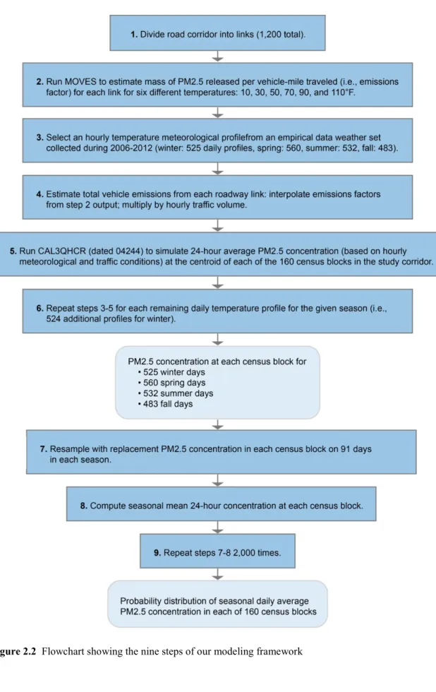
Our modeling framework includes nine steps (Figure 2.2):
Step 1: Divide roadway into links for analysis. Air emissions from any single vehicle depend substantially on the vehicle speed, vehicle acceleration, time spent idling, and road grade. To account for these effects, we followed the approach of Ritner et al. by dividing the study corridor roadway into very short links [10]. In total, we modeled 1200 links along the 8.2 km (5.1 mile) study corridor. Each link has a roughly constant road grade; fraction of vehicle time spent decelerating, idling or accelerating; and moving speed. We used ArcGIS 9.3.1 (ESRI, Redlands, CA) and 2010 aerial photos from the Orange County Geographic Information Systems (GIS) Division to draw the series of links [17]. Link-specific traffic activities were determined based on the simulated traffic data for 2009, 2025 no-build, and 2025 build scenarios from the transportation impact analysis [14]. Link-specific average speeds were assumed to be equal to speed limits based on GIS street maps from the Town of Chapel Hill [18]. The speed limit was 25 mph for 17% of the links, 35 mph for 68% of the links, and 45 mph for the remaining 15%. Link-specific grades were derived from GIS contour maps from the Town of Chapel Hill [19] and ranged from 0%–10%.
Step 2: Estimate vehicle emissions factors for six different temperatures for each link using MOVES. As suggested by both Ritner et al. [10] and the U.S. Environmental Protection Agency’s (EPA) “Guidance on Quantitative PM Hot-Spot Analyses for
Transportation Conformity” [20], we used MOVES 2010b (Motor Vehicle Emission Simulator, EPA, Washington, DC) to develop 2009 and 2025 link-specific emission rates of PM2.5
emissions from different kinds of vehicles under conditions designed to represent typical driving behaviors. Unlike its predecessor, known as MOBILE6, MOVES can provide separate emissions factors for different vehicle operation modes: acceleration, deceleration, idling, and cruising [10].
The EPA’s PM hot-spot guidance recommends that the link-specific emission rates should be prepared based on average temperatures for four different time periods in a day for each season, meaning that each development scenario would require 16 MOVES runs. However, this approach does not fully account for daily temperature variability within a given season. Previous studies have shown that PM emission rates are highlight sensitive to temperature, and hence omitting temperature variability could decrease the accuracy of modeled emissions factors [22, 23]. Our new algorithm for representing intra-seasonal variability in temperature and
meteorological conditions runs MOVES for six different temperatures: 10, 30°F, 50°F, 70°F, 90°F, and 110°F [23]. Later steps of the algorithm (described below) interpolate between these six estimates to determine temperature-specific emissions factors for each roadway link. For example, if a wintertime simulation of any given hour yielded a temperature of 40°F for that hour, we then estimated the vehicle emissions factors to be the average of the emissions factors for 30 and 50 degrees.
then we repeated this selection (step 6) without replacement 2099 times until we had estimated PM2.5 concentrations in each census block for each day having a complete weather record.
Step 4: Estimate the total emissions from vehicles traveling on each roadway link. The MOVES model estimates average per-vehicle emissions in grams per vehicle-mile,
accounting for the specific distribution of vehicle types, ages, and fuel sources at the study site. The next step was to compute the total mass of PM2.5 emitted from each vehicle on each roadway link. For this step, vehicle counts were needed. The link-specific traffic volumes were based on the simulated traffic data for 2009, 2025 no-build, and 2025 build scenarios from the Carolina North Traffic Impact Analysis [14]. For the temperature profile selected in step 3, we estimated emissions factors by interpolating between the outputs of step 2 for the nearest two temperatures.
Step 5: Model dispersion of PM2.5 from roadway emissions into the surrounding neighborhoods using CAL3QHCR. The PM hot-spot guidance suggests two air pollution dispersion models—CAL3QHCR (EPA, Research Triangle Park, NC) or AERMOD (EPA, Research Triangle Park, NC)—for simulating PM2.5 pollution dispersion from roadways. Both
Winter Spring
Summer Fall
Figure 2.4 Seasonal wind roses from 6 a.m. to 7 p.m., according to the meteorological data used in the CAL3QHCR modeling
perform better than AERMOD for analyses at the urban project scale [26]. In this study, we tested and used CAL3QHCR for estimating population exposure to PM2.5 (μg/m3) from the study corridor. As described below under “model validation approach,” we tested two different versions of CAL3QHCR: one dated 13196 and the other dated 04244. We then used the best-performing of the two in subsequent simulations. We ran CAL3QHCR for each roadway link using the meteorological profile from step 3 and the per-link total PM2.5 emissions from step 4. We modeled concentrations at an elevation of 1.5 m, corresponding to the elevation of the adult breathing zone.
Steps 6-9: Generate probability distribution of seasonal average 24-hour PM2.5 concentration. As Figure 2.2 outlines, we first repeated steps 3–5 for each of the days (2,100 in total) for which historical empirical weather data were available. The result was 2,100 separate daily estimates of the PM2.5 concentration at each of the 160 census block centroids: 525 winter day estimates and 560, 532, and 483 spring, summer, and fall estimates, respectively. We then used a bootstrap technique to estimate a probability distribution for the average daily PM2.5 concentration in each season. Specifically, for each season, we resampled with replacement 91 days from the simulated daily PM2.5 concentration estimates. We then computed the mean value of these 91 daily estimates for each receptor. Then, we repeated this process of computing a seasonal mean 1,999 times, in order to generate a sample of 2,000 seasonal mean 24-hour PM2.5 concentrations. This sample then served as the basis for developing a probability distribution of the mean concentration for each season.
Model Validation Approach
along the study corridor (Figure 2.1). Furthermore, we compared the predictive validity of two versions of CAL3QHCR (dated 04244 and dated 13196) According to the model change bulletin, the mixed mode rounding in the internal calculations of CAL3QHCR dated 04244 was removed from CAL3QHCR dated 13196. Consequently, the simulated concentrations from these two model versions are different in some cases.
We used a DustTrak DRX Aerosol Monitor Model 8534 (TSI, Shoreview, MN) to measure total PM2.5 concentrations at each of the three sites The DustTrak DRX instrument or similar models have been used in roadside measurements in several previous studies [27–29]. The DustTrak can detect concentrations from 1 to 150,000 μg/m3 with an error of ±0.1% of the monitored concentration [30]. All of these instruments are calibrated at the factory with a known mass concentration of Arizona Test Dust (ISO 12103-1, A1 test dust) [31]. In addition, in each sampling period, we calibrated the instrument before taking measurements. During all sampling events, the DustTrak was held about 1.5 m above the ground (the adult breathing zone height) and programmed to record the total concentration every five seconds.
from the roadway (except at Site 2, where obstructions prevented sampling at 50 m). Then, we repeated this process over the course of about one hour. As a result, at each site and during each sampling event, we collected PM2.5 concentrations for six three-minute intervals at 10 m, 30 m, and 50 m perpendicular distances from the roadway, as Figure 2.5 illustrates. For each event, we then computed the average PM2.5 concentration measured during these three-minute intervals; Table 2.1 shows the resulting estimated one-hour average concentrations.
During each sampling event, we simultaneously collected traffic counts and meteorological data. Traffic was monitored with a hand-held counter, and the counts were confirmed by viewing digital video recordings from a portable video recorder positioned on a tripod to film the roadway during sampling. We measured wind speed using a Skymate model SM-18 wind meter with accuracy within 3% (Campbell Scientific, Inc, Logan Utah); wind direction using a windsock and compass; and temperature, dewpoint, and relative humidity using an Extech model 445814 thermometer-psychrometer with temperature accuracy of ±1.8° F and relative humidity accuracy of ±4%. Data on atmospheric stability class and mixing height were estimated using EPA’s Meteorological Processor for Regulatory Models. Table 2.2 shows the traffic counts and meteorological conditions for each sampling event.
The measured concentrations at each sampling point represent the sum of background concentrations, PM2.5 contributions from other nearby sources, and traffic-related PM2.5. Therefore, in order to evaluate the performance of the CAL3QHCR model, concentrations of PM2.5 attributable to background and other sources must be subtracted from the monitored concentrations, in order to determine how much of the measured PM2.5 comes from the roadway. In testing model performance, other studies have used background concentrations measured at an upwind location or central air quality monitor [26, 32, 33]. However, Chapel Hill does not have an active PM2.5 monitor; the nearest PM2.5 monitor is about 45 km away, in Raleigh. Furthermore, due to resource limitations, we were able to use only one DustTrak monitor and hence were unable to capture background concentrations while simultaneously measuring near-road concentrations. Hence, we accounted for the effect of background PM2.5 by characterizing the differentials between the measured concentrations at pairs of sampling points at distances 10 m and 30 m, 10 m and 50 m, and 30 m and 50 m from the roadway. Table 2.1 shows these differentials, as computed from the measured concentrations.
A factor-of-two plot has been commonly used to evaluate the performances of the
CALINE series of dispersion models (e.g., CALINE3, CAL3QHC/CAL3QCHR, and CALINE4) [26, 32–35]. That is, modeled PM concentrations are plotted against measured concentrations to see whether the model estimates are within a factor of two of measured concentrations.
Data Cleaning
In total, the sampling events shown in Table 2.1 yielded 29 data points. Of these, five points had to be eliminated because the wind direction was outside of a 120° degree arc from a line drawn perpendicular to the roadway (see Figure 2.5). In such conditions, the monitoring locations were not downwind of the roadway and therefore could not capture roadway
contributions to PM2.5 [36]. Four additional data points were eliminated because they indicated negative dispersion (that is, PM2.5 concentrations increased rather than decreased with distance from the roadway). This data cleaning process left 20 data points for comparing measured PM2.5 concentrations to modeled concentrations.
Table 2.1 Measured and predicted PM2.5 concentrations (g/m3)
Site Date Time period Measured concentrations* Measured concentration difference** Predicted concentration differences: CAL3QHCR (dated 04244) Predicted concentration differences: CAL3QHCR (dated 13196)
10 m 30 m 50 m
10 vs. 30 m 10 vs. 50 m 30 vs. 50 m 10 vs. 30 m 10 vs. 50 m 30 vs. 50 m 10 vs. 30 m 10 vs. 50 m 30 vs. 50 m 1
16-May
Morning 14.9 13.8 13.9 1.1 1 NEG 0.7 0.9 0.2 0.7 1 0.3
Noon 9 8.7 8.3 0.3 0.7 0.4 0.5 0.8 0.3 0.4 0.6 0.1
Evening 9.7 10 9.7 NEG NEG 0.3 1 1.3 0.3 0.9 1.3 0.3
31-May
Morning 5.1 5.1 4.9 0 0.2 0.2 0.7 0.8 0.1 0.7 0.9 0.2
Noon 2.6 2.2 1.6 0.4 1 0.6 0.5 0.8 0.3 0.5 0.6 0.2
Evening 3 2.6 2.4 0.4 0.6 0.2 1.1 1.4 0.3 1 1.3 0.4
2 24-Apr
Morning 21.4 20.8 NA WD NA NA 0.5 NA NA 0.5 NA NA
Noon 10.5 10.4 NA WD NA NA 0.7 NA NA 0.6 NA NA
3 16-Apr
Morning 10.8 10.8 10.5 NEG 0.3 0.3 0.7 0.9 0.2 0.6 0.8 0.2
Noon 9.7 9.2 9 0.5 0.7 0.2 0.6 1 0.4 0.5 0.7 0.2
Evening 9.2 8.9 8.5 WD WD WD 0 0 0 0.1 0.1 0
* NA indicates PM2.5 could not be measured at this location due to a physical obstruction.
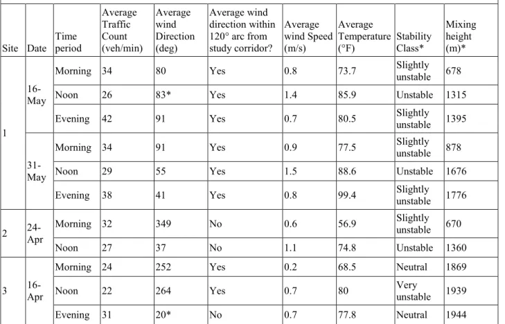
Table 2.2 Traffic and meteorological data used in CAL3QHCR modeling
Site Date Time period Average Traffic Count (veh/min) Average wind Direction (deg) Average wind direction within 120° arc from study corridor? Average wind Speed (m/s) Average Temperature (°F) Stability Class* Mixing height (m)* 1 16-May
Morning 34 80 Yes 0.8 73.7 Slightly
unstable 678
Noon 26 83* Yes 1.4 85.9 Unstable 1315
Evening 42 91 Yes 0.7 80.5 Slightly
unstable 1395
31-May
Morning 34 91 Yes 0.9 77.5 Slightly
unstable 878
Noon 29 55 Yes 1.5 88.6 Unstable 1676
Evening 38 41 Yes 0.8 99.4 Slightly
unstable 1776
2 24-Apr
Morning 32 349 No 0.6 56.9 Slightly
unstable 670
Noon 27 37 No 1.1 74.8 Unstable 1360
3 16-Apr
Morning 24 252 Yes 0.2 68.5 Neutral 1869
Noon 22 264 Yes 0.7 80 Very
unstable 1939
Evening 31 20* No 0.7 77.8 Neutral 1944
Wind speeds below 1 m/s were reset to 1 m/s when used in the CAL3QHCR modeling, as suggested in EPA’s Meteorological Monitoring Guidance for Regulatory Modeling Applications [37].
* Data obtained from MPRM.
Results
Vehicle Emission Rates
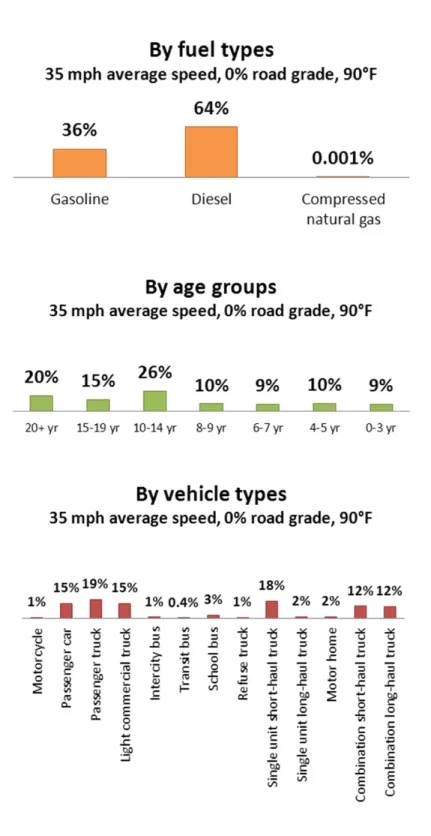
The output from MOVES can provide useful insights about the vehicle classes
contributing most to roadside pollution, the effects of meteorological and road characteristics on per-vehicle emissions, and the effects of future vehicle technologies.
various kinds of commercial trucks. Consistent with this result, diesel-fueled vehicles account for nearly two-thirds (64%) of emissions whereas gasoline-fueled vehicles account for 36%. As well, vehicles more than 10 years old account for half of the roadside emissions. Hence, improving emissions controls or engine efficiency in diesel-fueled trucks, plus retiring older vehicles, could greatly reduce roadside emissions in the study corridor.
MOVES output also shows the important effects of temperature, road grade, and vehicle speed on roadway emissions. As Figure 2.7 shows, emissions decrease as temperature increases, increase as road grade increases, and decrease as vehicle speed increases. These results illustrate the importance for modeling of accurately capturing temperature, vehicle speed, and especially road grade—hence the importance of dividing a study corridor into short links as in our study.
Model Performance Evaluation
Figure 2.8 compares the predictions of the two CAL3QHCR model versions to measurements of pollutant dispersion along the roadway corridor. The figure also shows the “factor-of-two envelope:” that is, the range of predictions that are within a factor of two of the measured dispersion. As shown, the models contain both under-predictions of the amount of dispersion (i.e., data points below the factor-of-two envelope) and over-predictions (data points more than twice the measured amount). However, both models are more likely to over-predict than to under-predict dispersion: that is, to predict greater concentration differences as one moves away from the roadway than were actually measured. Possible reasons for this prediction error include physical obstacles to dispersion (for example, at site 3, a large rock outcropping may interfere with dispersion) and intermittent winds. Previous model evaluations also have observed that the predecessor to CAL3QHCR did not perform well in the presence of street canyons or other physical obstacles or when winds are intermittent [32].
Estimated PM2.5 Exposure under Current and Future Scenarios
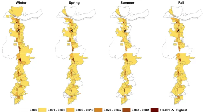
Our modeling approach can be used to predict the effects of the Carolina North campus on ambient PM2.5 concentrations in census blocks in the study corridor if the campus is built.
Even if the new campus is built, the roadway contribution to ambient PM2.5 levels in the study corridor is predicted to be very low by 2025. The maximum contribution of traffic to any one census block occurs in winter and is predicted to be 0.11 μg/m3, which is quite low in comparison with the ambient air quality standard (12 μg/m3 annual average PM2.5
concentration). In comparison, if the new campus is not built, the maximum PM2.5
concentration in any one census block is 0.085 μg/m3, which is 24% lower than if the campus is
built. In both cases, though, the maximum concentration is higher under current conditions than under future conditions, despite the anticipated traffic growth. Under current conditions, the model predicts that the maximum roadway contribution to seasonal PM2.5 in any one census block is 0.14 μg/m3, which is 24% higher than expected in 2025, even if the new campus is built. These future emissions reductions reflect the built-in assumptions of MOVES that the future vehicle fleet will become more efficient (less polluting) and that fuels will be cleaner. The results thus illustrate the value of ensuring continued improvements in vehicle fuel economy and
emissions standards.
Our modeling approach included a new method for representing meteorological
variability. Our results illustrate that variability can be important in some locations. Overall, the daily meteorological variability caused little change in seasonal daily mean PM2.5
concentrations. For example, in the 2025 scenario in which the Carolina North campus is built, the average coefficient of variation (i.e., standard deviation of the predicted seasonal mean divided by average of the seasonal mean) is 0.06, meaning that seasonal variability on average has a relatively small effect on model predictions. The maximum coefficient of variation in this scenario was less than 0.5, which means that 95% of the time, meteorological variability will change the predicted seasonal mean by less than a factor of 2. (According to the Central Limit Theorem, the seasonal mean converges to a normal distribution, and hence 95% of the time, the seasonal mean should be within two standard deviations of the actual mean, and in this case the standard deviation is about half the mean.) Thus, this meteorological variability is less important than the model uncertainty shown in Figure 2.8.
The modeling approach can be used to characterize spatial variability in roadway emissions effects on surrounding neighborhoods. Figure 2.9 shows the resulting spatial variability for current conditions, and Figure 2.10 shows the spatial variability for future
conditions. In both instances (because both models rely on the same set of meteorological data), the census block with the maximum concentration is in the same location and also (despite changes in wind directions) does not vary seasonally. The most affected census block (shown with arrows in Figures 2.9 and 2.10) is located on the east side of Martin Luther King Jr. Boulevard at Blossom Lane. Such information could be useful for zoning decisions (e.g., decisions about locations for schools, retirement homes, or other land uses attracting sensitive populations).
Discussion
Our results are consistent with the few empirical evaluations of the accuracy in predicting roadway PM2.5 concentrations of CAL3QHCR and its predecessor, known as CALINE. Yura et al. compared CALINE predictions of PM2.5 to measured PM2.5 concentrations at a busy
envelope for 69% of the Sacramento data points and for 59% of the London data points. In both cities, CAL3QHC outperformed CALINE. Gokhale and Raokhande compared the CALINE and CAL3QHC models’ ability to predict roadside PM2.5 concentrations at a busy intersection in Guwahati, India [38]. They found that the CAL3QHC model predictions were within a factor-of-two envelope for 65% of (66 of 102) hourly PM2.5 observations during winter and that the CAL3QHC model outperformed the CALINE model (the latter of which produced predictions within the factor-of-two envelope for 46 of 102 data points).
Our findings about the amount of PM2.5 contributed to a given location by a single busy roadway also are consistent with findings of the few modeling studies and quantitative HIAs of local effects of traffic in the United States. In a modeling study, Zhang and Batterman used CALINE along with the predecessor to MOVES, known as MOBILE6.2, to estimate the amount of PM2.5 pollution contributed by a busy roadway in Detroit, Michigan [33]. They found that the local roadway contributed only a small amount of the measured PM2.5: total measured PM2.5 concentrations averaged 16.8 μg/m3, but Zhang and Batterman attributed “no more than 0.5 μg/m3” to the roadway. They attributed the majority of observed PM2.5 “to long range transport of sulfate and other aerosols from the Ohio River Valley.” Chen et al. also found that roadways in Sacramento and London contributed relatively small fractions to observed PM2.5
concentrations at the study sites [26].
maximum predicted concentration in any census block in the study corridor is 0.7 μg/m3. This is within the range of concentrations predicted in the California studies.
Conclusions
In this study, a new modeling framework to quantify the project traffic growth impacts on population exposure to PM2.5 air pollution was proposed and then demonstrated by quantifying exposure to roadway PM2.5 emissions that may occur in the future due to the Carolina North development in Chapel Hill, North Carolina. This modeling framework should benefit others conducting quantitative HIAs of the built environment and transportation projects. Whereas previous HIAs employing air dispersion models have used average meteorological data and have assumed that vehicles move at a constant cruising speed along roadway links, our approach considers link- by-link variation in vehicle behavior and hourly meteorological variability.
Our results reveal that improvements in vehicle technologies and fuels will be a key factor in protecting public health from the air pollution generated by increases in traffic expected to occur due to local and regional developments in the future. In fact, the models we employed predict that traffic-related PM2.5 in the study corridor may actually decrease in the future, even if traffic increases, due to improved vehicle technologies and fuels.
Our results also reveal the need for improve models to predict near-road PM2.5
REFERENCES
[1] J. Kemm, “Perspectives on Health Impact Assessment,” Bull. World Health Organ., vol. 81, no. 6, p. 387, 2003.
[2] National Research Council, Improving Health in the United States: The Role of Health
Impact Assessment. Washington, DC: The National Academies Press, 2011.
[3] A. Wernham, “Health Impact Assessments are Needed in Decision Making about
Environmental and Land-Use Policy,” Health Aff. (Millwood)., vol. 30, no. 5, pp. 947–56, 2011.
[4] R. Lozano, M. Naghavi, K. Foreman, S. Lim, K. Shibuya, V. Aboyans, …, and C. J. L. Murray, “Global and Regional Mortality from 235 Causes of Death for 20 Age Groups in 1990 and 2010: A Systematic Analysis for the Global Burden of Disease Study 2010,”
Lancet, vol. 380, no. 9859, pp. 2095–128, 2012.
[5] A. L. Dannenberg, R. Bhatia, B. L. Cole, S. K. Heaton, J. D. Feldman, and C. D. Rutt, “Use of Health Impact Assessment in the U.S.: 27 Case Studies, 1999-2007,” Am. J. Prev.
Med., vol. 34, no. 3, pp. 241–56, 2008.
[6] M. Wismar, J. Blau, K. Ernst, and J. Figueras, “The Effectiveness of Health Impact Assessment: Scope and Limitations of Supporting Decision-Making in Europe,” Copenhagen Ø, Denmark.
[7] R. Bhatia and M. Katz, “Estimation of Health Benefits From a Local Living Wage Ordinance,” Am. J. Public Health, vol. 91, no. 9, pp. 1398–402, 2001.
[8] L. Singleton-baldrey, “The Impacts of Health Impact Assessment: A Review of 54 Health Impact Assessments, 2007-2012,” University of North Carolina at Chapel Hill, 2012. [9] R. Bhatia and E. Seto, “Quantitative Estimation in Health Impact Assessment:
Opportunities and Challenges,” Environ. Impact Assess. Rev., vol. 31, no. 3, pp. 301–309, 2011.
[10] M. Ritner, K. K. Westerlund, C. D. Cooper, and M. Claggett, “Accounting for Acceleration and Deceleration Emissions in Intersection Dispersion Modeling Using MOVES and CAL3QHC,” J. Air Waste Manage. Assoc., vol. 63, no. 6, pp. 724–736, 2013.
[13] K. Ross, “Carolina North Hearing Highlights Traffic Impact,” The Carrboro Citizen, 2009. http://www.carrborocitizen.com/main/2009/05/14/carolina-north-hearing-highlights-traffic-impact/.
[14] Vanasse Hangen Brustlin Inc., “Transportation Impact Analysis for the Carolina North Development,” Watertown, MA, 2009.
[15] Health Effects Institute, “Traffic-Related Air Pollution: A Critical Review of The Literature on Emissions, Exposure, and Health Effects, HEI Special Report 17,” Boston, MA, 2010.
[16] US Census Bureau, “Census Block Shapefiles with 2010 Census Population and Housing Unit Counts,” 2011.
[17] Orange County, “Aerials2010,” 2012.
[18] Town of Chapel Hill, “Street Centerline,” 2009. [19] Town of Chapel Hill, “2ft Elevation Contours,” 2009.
[20] US Environmental Protection Agency, “Guidance on Quantitative PM Hot-Spot Analyses for Transportation Conformity,” 2011.
http://www.epa.gov/otaq/stateresources/transconf/policy/pm-hotspot-guide.pdf.
[21] N.C. Division of Air Quality, “MOVES Input and Output Files: Hickory and Triad PM2.5 Redesignation Demonstration and Maintenance Plan,” 2011. .
[22] P. A. Mulawa, S. H. Cadle, K. Knapp, R. Zweidinger, R. Snow, R. Lucas, and J.
Goldbach, “Effect of Ambient Temperature and E-10 Fuel on Primary Exhaust Particulate Matter Emissions from Light-Duty Vehicles,” Environ. Sci. Technol., vol. 31, no. 5, pp. 1302–1307, 1997.
[23] D. Choi, M. Beardsley, D. Brzezinski, J. Koupal, and J. Warila, “MOVES Sensitivity Analysis: The Impacts of Temperature and Humidity on Emissions,” in The MOVES
Workshop 2011, 2011.
[24] National Climatic Data Center, “Quality Controlled Local Climatological Data (QCLCD),” 2013.
[25] National Oceanic and Atmospheric Administration, “NOAA/ESRL Radiosonde Database,” 2013.
[27] M. G. Boarnet, D. Houston, R. Edwards, M. Princevac, G. Ferguson, H. Pan, and C. Bartolome, “Fine Particulate Concentrations on Sidewalks in Five Southern California Cities,” Atmos. Environ., vol. 45, no. 24, pp. 4025–4033, 2011.
[28] J. S. Wang, T. L. Chan, Z. Ning, C. W. Leung, C. S. Cheung, and W. T. Hung, “Roadside Measurement and Prediction of CO and PM2.5 Dispersion from On-Road Vehicles in Hong Kong,” Transp. Res. Part D Transp. Environ., vol. 11, no. 4, pp. 242–249, 2006. [29] Y. Wu, J. Hao, L. Fu, Z. Wang, and U. Tang, “Vertical and Horizontal Profiles of
Airborne Particulate Matter Near Major Roads in Macao, China,” Atmos. Environ., vol. 36, no. 31, pp. 4907–4918, 2002.
[30] TSI Inc., “Spec Sheet Model 8533/8534 DustTrak DRX Aerosol Monitor,” 2012. [31] TSI Inc., “DustTrak DRX Aerosol Monitor Theory of Operation (EXPMN-002),” 2012. [32] E. A. Yura, T. Kear, and D. Niemeier, “Using CALINE Dispersion to Assess Vehicular
PM2.5 Emissions,” Atmos. Environ., vol. 41, no. 38, pp. 8747–8757, 2007.
[33] K. Zhang and S. Batterman, “Near-Road Air Pollutant Concentrations of CO and PM2.5: A Comparison of MOBILE6.2/CALINE4 and Generalized Additive Models,” Atmos.
Environ., vol. 44, no. 14, pp. 1740–1748, 2010.
[34] P. E. Benson, “CALINE3, A Versatile Dispersion Model for Predicting Air Pollutant Levels Near Highways and Arterial Streets,” Sacramento, CA, 1979.
[35] P. E. Benson, “CALINE4, A Dispersion Model for Predicting Air Pollutant Concentrations Near Roadways,” Sacramento, CA, 1989.
[36] Battelle, “Detailed Monitoring Protocol for US 95 Settlement Agreement,” Columbus, OH, 2006.
[37] US Environmental Protection Agency, “Meteorological Monitoring Guidance for Regulatory Modeling Applications, EPA-454/R-99-005,” Research Triangle Park, NC, 2000.
[38] S. Gokhale and N. Raokhande, “Performance Evaluation of Air Quality Models for Predicting PM10 and PM2.5 Concentrations at Urban Traffic Intersection During Winter Period,” Sci. Total Environ., vol. 394, no. 1, pp. 9–24, 2008.
CHAPTER 3
HEALTH IMPACT ASSESSMENT OF TRAFFIC-RELATED AIR POLLUTION AT THE URBAN PROJECT SCALE:
INFLUENCE OF VARIABILITY AND UNCERTAINTY2
Introduction
In the United States, nonprofit organizations and public health practitioners increasingly advocate for formal health impact assessments (HIAs) to inform land-use and transportation planning decisions [1, 2]. Signaling the heightened interest in HIAs in the United States, the U.S. National Academy of Sciences in 2011 published a report, Improving Health in the United
States: The Role of Health Impact Assessment, concluding that “HIA is a particularly promising
approach for integrating health implications into decision-making” [3]. The report offered the following formal definition of HIA:
“HIA is a systematic process that uses an array of data sources and analytic methods and considers input from stakeholders to determine the potential effects of a proposed policy, plan, program, or project on the health of a population and the distribution of those effects within the population. HIA provides recommendations on monitoring and managing those effects.”
substantial changes to decision-making processes in arenas outside the traditional healthcare sector. For example, decisions by transportation and municipal planning organizations can promote or limit opportunities for physical activity and can exacerbate or decrease exposure to ambient air pollution. While HIAs have been used in Europe, Australia, Canada, and Thailand for decades, the first U.S. HIA was completed in 1999 by the San Francisco Department of Public Health [2, 3]. By the end of 2012, however, at least 115 U.S. HIAs had been completed, and another 64 were under way [4]. Of the completed HIAs, 70 (more than 60%) focused on proposed changes to the built environment and/or transportation networks [4, 5].
To have maximum impact on land-use and transportation decisions, HIAs ideally would provide quantitative estimates of the health effects of the decision alternatives under
consideration. That is, they would estimate the number of deaths and illnesses prevented or caused by each alternative. This information then could be used to quantify the health costs (positive or negative) of each alternative. Such quantitative cost and benefit estimates are needed, because cost-benefit analysis drives major transportation and land-use decisions in the United States [6]. However, only 5 of the 70 transportation-related HIAs in the United States carried out prior to 2013 quantified the expected health impacts [4, 7]. Table 3.1 summarizes these HIAs. The remaining HIAs expressed qualitative conclusions.
work, or visit within the air-shed of the affected streets.” The HIA recommended several mitigation measures to reduce air pollution exposures: congestion pricing, increased public transit, zoning of sensitive uses away from roadways, and vegetation buffers around roadways. The HIA did not quantify the air quality or health impacts of the proposed new development or these mitigation alternatives.
While the above-mentioned five previous quantitative HIAs estimate the magnitude of air quality and related health impacts, none considers the potential variability and uncertainty of the estimates. Rather, these HIAs each provide a single, deterministic prediction of traffic-related air quality and health impacts for each decision option (see Table 3.1). The reliance on
deterministic estimates is a major limitation because it fails to consider the full range of potential risks, including, for example, impacts on highly exposed or vulnerable populations or impacts under extreme weather conditions. The deterministic approach also fails to provide information to decision-makers about the degree of certainty in the predictions. Box 3.1 highlights
potentially important sources of variability and uncertainty. Previous quantitative HIAs have not considered the effects of these uncertainty and variability sources on their health impact
estimates.