i
Hydraulic analysis of stream restoration on flood wave propagation
Joel Sholtes
A thesis submitted to the faculty of the University of North Carolina at Chapel Hill in partial fulfillment of the requirements for the degree of Master of Arts in the Department of Geography.
Chapel Hill
2009
Approved by:
Martin W. Doyle, Ph.D.
Lawrence E. Band, Ph.D.
ii Abstract
Joel Sholtes
Hydraulic analysis of stream restoration on flood wave propagation (Under the direction of Martin Doyle, Ph.D.)
Channel and floodplain restoration can enhance the ability of a channelized or incised reach
to temporarily store the flow and dissipate the energy of passing flood waves. Elements of restoration
design that can enhance flood wave attenuation include the introduction of meanders, which reduces
channel slope and increases channel length, restoring channel-floodplain connectivity, and
re-vegetating banks and the floodplain. I examined the efficacy of stream restoration to attenuate floods
given the scale at which it occurs and the magnitude of channel change possible by quantifying flood
wave attenuation on two restored reaches located in urban and rural catchments and on hypothetical
stream reaches representing median values of stream restoration projects in North Carolina using a
dynamic flood routing model (UNET in HEC-RAS). Floods routed in impaired and restored reach
models of field sites either exhibited very small augmentation to attenuation, largely due to assumed increases in floodplain roughness, or a decrease in attenuation. Modeled sensitivity results indicated
that decreases to slope and increases to channel and floodplain roughness demonstrated the highest
relative impact to attenuation. Floods of intermediate magnitude (between 2 and 5 yr recurrence
interval) were impacted most by restoration, especially those confined to the channel under the
iii
Acknowledgements
I would like to thank my fiancée Kari Leech for her support in the field and at home and for being by my side through both the glades and the bogs of graduate school. Martin Doyle, my advisor, helped develop the research goals and questions for this work, provided technical support, reviews, and the necessary kicks in the pants along the way. He has been an honest, available, and effective advisor. I thank my Master’s committee members Larry Band and Brian White for their guidance and feedback throughout this process. Jeffrey Muehlbauer and Daisy Small, my colleagues in the Doyle Lab, provided reviews of this manuscript and were exceptional volunteers in the field. Sally Whisler, Benjamin Bogardus, and Autumn Thorye provided helpful field assistance at various points
iv
Table of Contents
1.0 INTRODUCTION ... 1
1.1 Stream Restoration and Flood Attenuation ... 1
1.2 Modeling Flood Attenuation ... 3
2.0 DATA & METHODS... 7
2.1 Methods and Analysis Overview ... 7
2.2 Flood Routing in Hypothetical Reaches ... 8
2.2.1 Stream Restoration Parameter Data ... 8
2.2.2 Stream Morphology Sensitivity Analysis ... 10
2.2.3 Synthetic Hydrograph Generation... 10
2.3 Unsteady Flow Numerical Model... 12
2.3.1 Model Description & Discussion ... 12
2.3.2 Model Parameterization and Assumptions ... 12
2.4 Field Data Collection and Reach Model Creation ... 13
2.4.1 Study Reach Characterization ... 13
2.4.2 Hydraulic Measurement at Field Sites ... 16
2.4.3 Study Reach Model Calibration ... 17
2.4.4 Flood and Hydrograph Preparation ... 18
2.4.5 Unit Hydrograph Generation ... 19
2.4.6 Flood Routing Comparison Between Restored and Impaired Reaches ... 20
3.0 RESULTS ... 21
3.1 Attenuation for Hypothetical Channel Restoration ... 21
3.2 Flood Wave Attenuation and Channel Design Elements Sensitivity Analysis ... 23
3.3 Study Site Field Data and Modeling... 24
3.3.1 Converted and Routed Hydrograph Comparison ... 24
3.3.2 UT South Fork Modeled Flood Routing ... 28
v
4.0 DISCUSSION ... 31
4.1 The Effect of Stream Restoration on Flood Wave Attenuation ... 31
4.1.1 Study Reach Models ... 31
4.1.2 Hypothetical Reach Models ... 33
4.1.3 Demonstration of Enhancement to Attenuation ... 34
4.2 Viability of Restoration in Attenuation Enhancement ... 36
4.2.1 Previous Work ... 36
4.2.2 Channel and Floodplain Properties Significant to Attenuation ... 37
4.2.3 Conditions for Enhancement to Attenuation ... 38
4.3 Kinematic Celerity Analysis Channel Restoration Design ... 38
5.0 CONCLUSION ... 43
6.0 TABLES ... 46
7.0 FIGURES ... 53
8.0 APPENDIX A: Hypothetical Impaired and Restored Reach Parameter Data ... 75
9.0 APPENDIX B: TR-55 Method and Synthetic Unit Hydrograph Generation ... 82
10.0 APPENDIX C: Model Calibration and Computational Parameter Sensitivity Analysis ... 87
11.0 APPENDIX D: Hydraulic Measurements at Field Sites and Field Site Characterization ... 92
12.0 APPENDIX E: Unit Hydrograph Generation for UT South Fork ... 99
vi List of Tables
1. Summary of study data, methods, and terminology. ………..……….47 2. Summary statistics from sample of stream restoration projects that have occurred in
North Carolina under the Ecosystem Enhancement Program………...…………48
3. Hypothetical stream restoration parameters with sources of values.………....………...49
4. Channel and Floodplain parameter values for stream restoration design sensitivity
analysis. .……….……….……50
5. Study Reach Properties……….……….………..51
vii List of Figures
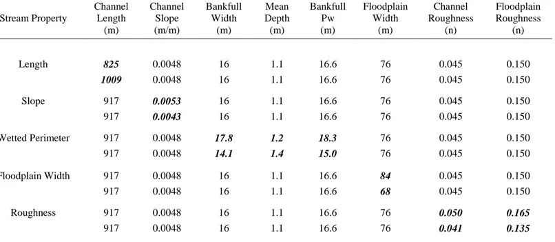
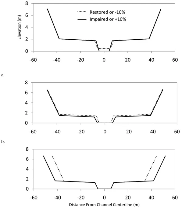
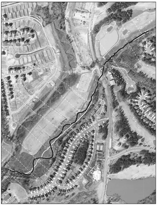
1a - c. Diagrams of channel and floodplain geometry used in hypothetical impaired and restored reach (a) and restoration design sensitivity (b & c) analyses.……….…...54 2a - b. Aerial photograph of restored study reaches with surveyed cross section cutlines,
restored channel outline, and impaired channel outline. .………55
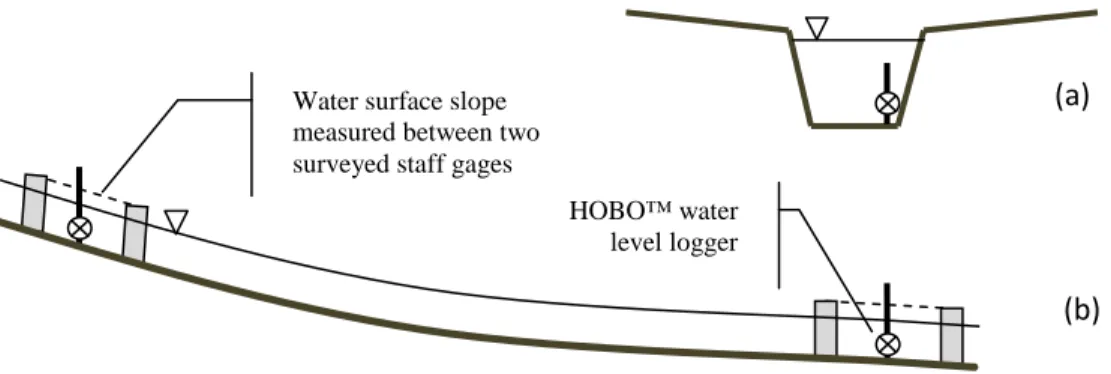
3a - b. Cross sectional (a) and longitudinal (b) schematic of equipment placement in study
reaches.……….…....……….…...57
4. Example of calibrating of HEC-RAS study reach models to best fit routed hydrographs to recorded hydrographs..……….…....………58
5a - b. Selected hydrographs as measured in the upstream cross section at UT South Fork
(a) and Smith Creek (b), then converted in discharge hydrographs in UNET………...59
6. Unit hydrograph generated from a 6 hr precipitation event at UT South Fork………60
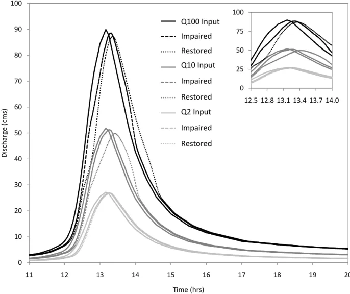
7. Comparison of input and output hydrographs in the impaired and restored channel reconfiguration scenarios for 24-hr synthetic hydrographs with return intervals of 100, 10, and 2 years. ……….…..….……….…....…………..………… 61
8a - d. Comparison between input and output hydrographs routed through impaired and restored hypothetical reaches at each flood return interval. ………….…..….……….…....…….62 9. Dimensionless changes to instantaneous peak discharge over dimensionless distance
downstream between hydrographs routed through hypothetical impaired and restored
reach models.……….…..….……….…....………...63
10a - b. Maximum water surface heights at the downstream station for 100, 50, 10, and 2 yr
floods routed through hypothetical impaired (a) and restored (b) reaches..………….…..…..64
11. Percent difference in Qpk between each scenario and the baseline condition represented by the hypothetical restored reach model across various flood frequencies..………..65
12. Comparison channel parameter scenarios by summing the differences in percent
reduction to Qpk between +10% and -10% conditions across all studied flood frequencies…66
13a - b. Comparison of duration of overbank flow and difference in average celerity
between +10% and -10% among all channel property scenarios and flood frequencies…...67
14a - f. Comparisons of converted and routed hydrographs between upstream and downstream stations and recorded and routed stage hydrographs at the downstream station for selected floods on
viii
15a - f. Comparisons of converted and routed hydrographs between upstream and downstream stations and recorded and routed stage hydrographs at the downstream station for selected floods on
Smith Creek..……….…..….……….…....……….…69
16a - c. Comparison of changes to Qpk, CAVG, and tOB in floods routed through impaired and
restored reach models of UT South Fork……….…..….……….…...70
17a - c. Comparisons of relative and absolute reduction to Qpk, and CAVG in floods routed
through impaired and restored reach models of Smith Creek……….…..…...71
18. Dimensionless instantaneous peak discharge over dimensionless distance downstream for three floods routed in pre-existing and restored reach models of UT South Fork. ………72
19a - d. Comparisons of relative (a) and absolute (b) reduction to Qp, CAVG, and tOB between up- and downstream stations for floods of various return intervals routed through impaired and restored reach models. ……….…..….……….…....……….73
ix
List of Symbols
A Cross sectional area of flow (m2) b Average channel width (m)
CAVG Average celerity (kmhr
-1
)
CK Kinematic celerity (kmhr
-1
)
g Gravitational constant (ms-2)
γ Specific weight (Nm-3)
n Manning’s coefficient of surface roughness (unitless)
P Wetted perimeter (m)
ρ Density (kgm-3)
θ Weighting factor in implicit numerical solution for St Venant Equations
Q Discharge (m3s-1)
Q2-Q100 Flood with two to 100 year recurrence interval
Qpk Instantaneous Peak Discharge (m3s-1)
So Slope of channel bed (m/m)
Sf Friction slope (m/m)
tOB Duration of overbank flow (hr)
v Streamwise velocity (ms-1)
x Streamwise distance (m)
1
1.0 INTRODUCTION
1.1 Stream Restoration and Flood Attenuation
Stream restoration is increasingly practiced throughout the US, mounting to a > $1 billion per
year industry (Bernhardt et al., 2005). Under Section 404 of the Clean Water Act, unavoidable
impacts to streams and wetlands must be mitigated by restoring streams and wetlands elsewhere,
termed compensatory mitigation (Hough & Robertson, 2009). Considerable resources are expended
on mitigating impacts from development in North Carolina. Since its inception in 1999 to 2007 the
North Carolina stream and wetland mitigation program (currently Ecosystem Enhancement Program,
EEP) has overseen the creation of over 400,000 m of mitigation credits for stream impacts. The
majority of this mitigation has been generated through stream restoration, with over $230 million
spent on stream and wetland mitigation (NCEEP, 2007). Stream restoration in North Carolina occurs
primarily through the EEP mitigation program, which utilizes guidelines for stream restoration
developed by the US Army Corps of Engineers based on the concepts of Natural Channel Design (Rosgen, 1997; US Army Corps of Engineers, 2003). Streams are restored for a variety of goals under
the general framework of reestablishing the functions of “undisturbed streams.” These include, but
are not limited to, maintaining water quality, providing habitat for aquatic species, and storing and
attenuating flood flows (FISWRG, 1998). The memorandum creating the EEP explicitly includes
flood attenuation stating that its mission is:
"… to protect and improve water quality, flood prevention, fisheries, wildlife and plant habitats, and recreational opportunities through the restoration, enhancement and preservation of wetlands and riverine areas within North Carolina's water basins…(§2,B p.3 Memorandum of Agreement between the NCDEP, NCDOT, and the ACOE, 2003)
Floods are attenuated in undisturbed streams through several mechanisms. During floods,
2
a river. Flood flows are detained within a stream channel throughout its length and in low, flood
prone areas (Dunne & Leopold, 1978). Woody debris (Shields & Gippel, 1995), meanders (Fares,
2000), and vegetation (Ghavasieh et al., 2006) within the channel and floodplain impact flood waves by reducing flow velocity and providing temporary storage of flood waters. A flood wave traveling
through a stream with these features will have its instantaneous peak discharge (Qpk), peak stage, and
celerity (wave speed, C) reduced as it moves downstream, assuming no inputs from tributaries. This
results in a downstream hydrograph that is longer in duration with a decreased Qpk. Flood attenuation
is a general term and can be quantified many ways. For the purposes of this study, attenuation will be
quantified by relative and absolute reductions to Qpk, with units of discharge (m
3
s-1), average celerity,
CAVG, with units of velocity (ms
-1
), and duration of overbank flow, tOB, with units of time (hr).
Direct or indirect modifications to stream channels that increase conveyance capacity can
reduce flood attenuation along a stream and cause floods to travel more quickly. Direct channel
modifications such as straightening, deepening, and widening (stream channelization or training)
increase conveyance by augmenting the volume of the stream per unit length, steepening its slope,
and reducing channel roughness. Comparison of flood hydrographs between adjacent straightened
and meandering streams (Doyle & Shields, 1998) and between before and after stream channelization
(Campbell et al., 1972; Shankman & Pugh, 1992; and Wyzga, 1993) demonstrated increases in
downstream Qpk, peak stage, and C. While stream channelization efforts reduce flooding locally, they
can increase flood hazard downstream. Channel modification resulting from indirect human impacts
such as incision and enlargement caused by increased catchment runoff from land use change (e.g.
Booth 1990, and Doll et al. 2002) or downstream changes to slope from channelization (Wyzga, 1993; and Doyle & Shields, 1998) can generate the same effect on floods.
One of the touted benefits of stream restoration is to reverse the effects of channelization and
incision by restoring a stream’s ability to slow down and retain flood waters (e.g. Acreman et al.,
2003; Campell et al., 1972; Liu et al., 2004). This may be accomplished through many aspects of
3
relative to valley slope. Vegetation may be re-introduced along the banks and within the floodplain.
Creation of a new channel with a floodplain at a lower relative elevation will allow floods of a certain
frequency to leave the channel and spread out into the floodplain where flood waters are slowed and temporarily stored. Conceptually, stream restoration has the potential to augment the ability of a
formerly incised reach to reduce Qpk and disperse flood waves via enhanced energy dissipation and
increased channel and floodplain storage capacity. However no studies to date have documented the
actual impact of reach-scale stream restoration on floods. As such, it is important to understand the
hydraulic contribution of stream restoration to flood wave propagation within a stream network.
1.2 Modeling Flood Attenuation
Modeling flood wave propagation and attenuation has been studied in the field of
computational hydrology and hydraulics for decades. Flood wave propagation refers to the
movement or routing of a flood through a river channel or network. Attenuation refers to the
reduction in peak and dispersion of the flood hydrograph as it propagates. Early computational flood
routing models, such as DAMBRK created by Fread (1982), simulate a flood wave caused by a dam
failure. DAMBRK and its more general successors solve the one-dimensional St.Venant equations
for unsteady flow in the stream wise direction (x):
0 (1)
(2)
Equation (1) is the continuity equation of mass with v as the velocity, A as the cross sectional area of
flow, and b as the channel width. Equation (2) is the dynamic or momentum equation with So and Sf
representing the channel bed and energy slopes, respectively. These equations are depth-averaged and
solved across the channel and floodplain cross section at each flow rate and time interval throughout
the flood hydrograph and stream reach. One-dimensional flood routing models that solve the full St.
4
momentum all the relevant dynamic forces acting on flow and account for attenuation due to drag and
local storage (Henderson, 1966). Other one-dimensional flow routing models include the kinematic
wave model, which does not account for wave attenuation, merely translation; and the diffusive wave model, which does not account for the momentum dynamics and pressure forces within a wave
(Chow et al., 1988).
One-dimensional modeling of flood wave propagation is used extensively; however, it does
not explicitly account for the two- and three-dimensional aspects of energy dissipation due to
turbulence exchange at the interface of floodplain and channel flows as momentum lost in transverse
flows around meander bends (Shiono, 1999; Knight, 2005). Increasingly complex two and three
dimensional models also exist using other forms of the St. Venant equations. These models are able to
explicitly account for the two and three dimensional flow patterns that occur within the channel
around meander bends and between the channel and floodplain. Though one-dimensional models lack
this capability, the energy losses associated with complex and transverse flows can be approximated
by the roughness coefficients used in calibrating one dimensional models, which are widely applied to
practical and theoretical questions associated with flood wave routing (Knight, 2005).
For the purposes of this study, a one-dimensional model will suffice in order to quantify the
relative change in flood wave attenuation between before and after restoration scenarios as well as for
the sensitivity analysis to stream and floodplain properties. The unsteady flow modeling component
of Army Corps of Engineers, Hydraulic Engineering Center, River Analysis System (HEC-RAS
Version 4.0; ACOE, 2008), UNET, developed by Barkua (1992) was used for dynamic flood routing
in this study. HEC-RAS is an industry standard numerical hydraulic model and is widely used among the stream restoration design community.
Previous modeling work has quantified the effects of various stream and floodplain properties
on the propagation of flood waves, though often over long distances. Wolff and Burgess (1994) used
a one-dimensional flood routing model to study the relative effects of channel slope, roughness, and
5
Reducing a channel’s slope, increasing its roughness, and providing flood waters access to rougher
floodplains increased a stream’s “effective storage,” which the authors attribute as the main driver of
flood attenuation. Ghavasieh et al. (2006) and Anderson et al. (2006) modeled the effects of various hypothetical vegetation arrangements along the channel and in the floodplain over 20 km and 50 km
reaches, respectively. Both studies found significant attenuation in modeled propagated floods which
varied according to the spatial arrangement of vegetation patterns. Ghavasieh et al. found that the
one-dimensional model tended to overestimate flood attenuation compared to the two-dimensional
model. Acreman (2003) focused his flood attenuation study on floodplain re-establishment at the 10
km scale, finding 10% to 15% reductions in Qpk using a one dimensional flood routing model.
Other work has measured the influences of channel and floodplain morphology on flood
attenuation through field and modeling studies. Woltemade (1994) found that incised channel
morphologies on mid-catchment reaches increased flood wave celerity. He modeled the effect of
removing the incised morphology on a watershed scale and documented augmented attenuation to
floods of moderate magnitude (5 to 25 yr recurrence interval floods) reasoning that larger floods (50
to 100 year recurrence interval) overwhelmed a stream’s ability to slow down and capture flood
waters and smaller floods largely remained within the channel where less attenuation occurs.
Turner-Gillespie et al. (2003) found that geologic conditions leading to wider valley bottoms and channels
with gentler slopes served to attenuate floods as measured along an 8 km reach. They documented
decreases to Qpk up to 48% in the field for the largest floods.
While the effects of various aspects of channel and floodplain properties on flood wave
attenuation have been studied in the field and within models, specific assessment of the impacts to flood waves of reach-scale channel change via restoration has not been explicitly considered. This
study uses measurements of floods routed through restored reaches in conjunction with a
one-dimensional dynamic flood routing model to quantify the effect of restoration on flood waves before
and after restoration. At question is whether channel and floodplain modification of the scale typical
6
attenuation including reductions to Qpk, CAVG, and tOB. The relative significance of restoration design
components on flood wave attenuation, changes in attenuation with increasing flood magnitude, and
the sensitivity of flood wave celerity to channel properties are all quantified.
In order to study the effect of stream restoration on flood wave attenuation, I first describe a
hypothetical case of stream restoration using channel design data from restoration projects conducted
in North Carolina that compares flood attenuation change between incised and restored channel
morphologies. I conducted a sensitivity analysis of the relative significance of various channel
properties on routed floods. In a field-based study of attenuation on restored reaches, I measured and
modeled the changes to flood attenuation brought on by two stream restoration projects. Finally, I
used a simple, theoretical relationship between kinematic celerity and channel properties to further
7
2.0 DATA & METHODS
2.1 Methods and Analysis Overview
I assessed the impact of channel reconfiguration on flood waves through field measurements and hydraulic modeling of actual and hypothetical conditions. The primary response variables used
in this study to quantify attenuation were changes to instantaneous peak discharge (Qpk) average
celerity (CAVG, distance between stations over peak to peak travel time), and duration of overbank
flow at the downstream station (tOB). The variables were chosen to quantify reductions in flood peak,
wave speed, and hydrograph dispersion, respectively.
I first compared the differences in attenuation among synthetic flood hydrographs of various
return intervals routed through hypothetical incised and restored reaches using the unsteady flow
component of HEC-RAS, UNET. I assessed the relative importance of hydraulically significant
design elements utilized in channel reconfiguration projects, including changes to channel length,
slope, cross section geometry, and floodplain characteristics, by varying the values of these elements
and assessing their relative impacts on routed flood waves.
Next, I measured flood wave attenuation in reconfigured channels at two field sites. I
developed and calibrated HEC-RAS models of the reaches in their current, restored and impaired
configuration and evaluated the changes to flood wave attenuation between the two morphologies. A
unit hydrograph was developed for one site and scaled for floods with return intervals greater than
those measured in the field (10, 25, 50, and 100 yr). The hydrographs were routed through each reach
model to assess how the difference in attenuation between the two channel morphologies changed with increasing flood magnitude. The field-based studies of flood routing provided context to the
8
exercise in hypothetical reaches and theoretical analysis of kinematic celerity. An overview of data,
methods, and terminology used in this study is provided in Table 1.
2.2 Flood Routing in Hypothetical Reaches
2.2.1 Stream Restoration Parameter Data
Two hypothetical stream reaches were developed to quantify changes to attenuation resulting
from median values of channel change associated with restoration: an “impaired” reach with incised
banks and a “restored” reach with a greater length and milder slope due to re-meandering, and a
greater width to depth ratio among other adjustments (Figure 1a). In order to understand the scale of
stream restoration and the magnitude of changes to channel and floodplain properties involved in
restoration, I used available data from a sample of restoration projects conducted through the EEP.
These values along with regional hydrology data and hydraulic geometry curves provided context for
the hypothetical impaired and restored reaches. The following details the sources of channel
parameter values and the rationalization for their use. To develop hypothetical reaches representing
the scale and geometry of impaired and restored streams in an urban setting in the North Carolina
Piedmont, I used several sources of data (see Appendix A).
The median value of length, drainage area, and slope for the hypothetical reaches were
gathered from EEP restoration project reports (EEP, 2007). Given the standardized method used in
stream restoration design in North Carolina, stream design parameters can be easily related among
different restoration sites. Based on this sample of restoration projects, the mean drainage area of a
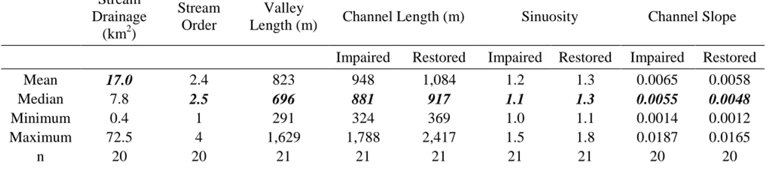
reach targeted for restoration is 17 km2, and the median length is 881 m with a slope of 0.55% (Table
2). After restoration, the median channel length is 917 m (4% increase) with a median slope of 0.48%
(12% reduction). Increasing stream sinuosity by introducing meanders results in increases to channel
length and decreases to channel bed slope. The bankfull width to mean depth ratio (W:D) increased from 10.7 to 12.9 and entrenchment ratio (ER, bankfull width to flood prone width) increased from
9
practice tends to target smaller streams (1st to 3rd Strahler order) and tends to increase channel length,
W:D, and ER while decreasing slope.
Median values of channel length, slope, and drainage area from EEP restoration projects, provided values for the hypothetical impaired and restored reach models (Table 3). The hypothetical
reaches were given trapezoidal channels set within floodplains with 1% lateral slopes leading up to
valley walls with 50% lateral slopes. Values for the cross sectional geometry of the impaired reach
was derived from regional hydraulic geometry curves developed for urban streams in the North
Carolina Piedmont (Doll et al. 2002) using the mean drainage area of restored stream sites as inputs
(17 km2). A 17 km2 drainage area yielded a bankfull discharge of 28 m3s-1 from these regional curves,
and resulted in channel geometry that would accommodate a discharge of 49 m3s-1 at top of bank
given the chosen slope. Urban streams are significantly enlarged in terms of channel cross section
area, width, and depth in comparison to rural streams. Bankfull discharge was estimated using
geomorphic features within the channel and is not necessarily the discharge that fills the banks,
especially in urban streams (Doll et al. 2002).
Cross section geometry values for the restored reach were chosen such that the channel would
be filled by the bankfull discharge (28 m3s-1) derived from the urban Piedmont hydraulic geometry
curves while maintaining a W:D greater than 12. Restored channels are generally designed to convey
a top of bank discharge equal to the channel forming discharge estimated by either bankfull
geomorphic channel features (Leopold 1995), an effective discharge calculation from hydrologic and
sediment transport data, or a specific flood frequency ranging from 1 to 2 yr (Doyle et al. 2007). A
W:D value of 12 along with an ER of 1.4 are guideline thresholds used in part to distinguish incised channels from non-incised channels according to the design guidance for restoration of incised
channels outlined by Rosgen (1997) utilized in North Carolina. Under this stream classification
framework, the impaired reach can be considered an incised “G” channel with W:D <12 and ER <1.4
and the restored reach a “C” channel with W:D >12 and ER>2.2, a common target morphology for
10
Manning's roughness coefficients for the impaired reach were chosen to represent a straight
lowland stream with some weeds and stones in the channel (n = 0.035) with a grassy floodplain (n =
0.05). Roughness values for the restored reach were chosen to represent a meandering stream of the same type (n = 0.045) with a forested floodplain containing undergrowth (n = 0.15) (Chow 1959).
Generally, stream restoration requires removing much of the pre-existing vegetation on the floodplain
for channel excavation. This serves to reduce floodplain roughness initially, so the roughness values
chosen for the restored hypothetical floodplain represent conditions that would exist several years
after restoration.
2.2.2 Stream Morphology Sensitivity Analysis
In addition to the difference in flood attenuation between hypothetical impaired and restored
reaches, the contribution of individual channel parameters to flood attenuation was of interest.
Stream slope (So), length, roughness (n), wetted perimeter, and floodplain width were all adjusted
±10% from the values used in the hypothetical restored reach (Table 4, Figures 1b & 1c, Appendix
A). By routing the same synthetic floods through these reach models and comparing changes in Qpk,
CAVG, and tOB, I quantified the relative importance of each stream property on flood wave attenuation.
Values of wetted perimeter were chosen such that the design discharge would fill the channel entirely
in all cases.
2.2.3 Synthetic Hydrograph Generation
I next needed a set of synthetic hydrographs to route through the hypothetical reach models.
Continuing with the approach of using parameters with values based on the scale and geometry of
restored urban channels in the North Carolina Piedmont, synthetic hydrographs were generated based
on a hypothetical catchment in an urban setting. Many synthetic hydrograph generation methods
exist. Some flood attenuation studies utilized the gamma distribution, in which the peak, time to peak, and skew can be defined (Wolff & Burgess, 1994; Anderson et al. 2006). However, the gamma
11
a more empirical synthetic hydrograph was desired. The TR-55 method was chosen due to its ease of
use and applicability to small urban catchments (NRCS 1986).
A 24 hr synthetic unit hydrograph with the mean drainage area of the sample restoration projects (17 km2) was generated using the TR-55 method. The unit hydrograph was converted to
flood hydrographs with return intervals of 2, 10, 50, and 100 yr (Q2, Q10, Q50, Q100) using equations
defining relationships between Qpk, drainage area, and impervious cover percentage developed by the
USGS (1996) for urban drainages in the North Carolina Piedmont and climatologic data from NOAA
(2006) providing precipitation depths for events with the same return intervals.
Input parameters for the TR-55 method include a defined catchment with measured drainage
area, land cover characteristics and percentages, and channel network lengths and slopes. Impervious
cover percentage for the hypothetical urban watershed was chosen such that the Q2 from the USGS
equation relating drainage area and impervious surface areas to Qpk matched the bankfull discharge
output of the urban Piedmont hydraulic geometry curve. Using this relationship, a 17 km2 drainage
area with an impervious surface coverage of 18% generates a Qpk of 28 m
3
s-1 at a return interval of
two years. An ovular-shaped catchment was assumed with one main channel and a mixture of
impervious cover (18%, CN=98) and grassed lawns in fair condition over hydrologic soil group B
(72%, CN=69).
Precipitation runoff depths with a 24 hr duration obtained from the NOAA Atlas 14 (2006) at
the defined return intervals were used to scale the unit hydrograph. Hydrographs generated with the
TR-55 method uniformly had greater Qpk at each return interval than the peaks generated by the
USGS equations. Each synthetic hydrograph was scaled by multiplying the hydrograph ordinates by the ratio of USGS to TR-55 generated Qpk at each return interval. This created hydrographs of the
12
2.3 Unsteady Flow Numerical Model
2.3.1 Model Description & Discussion
The numerical unsteady flow modeling component of HEC-RAS, UNET, developed by
Barkua (1992) was used to route the synthetic flood hydrographs through the hypothetical and field
site reaches models. This unsteady flow model provides a one-dimensional, implicit, finite-difference
approximation of the St. Venant equations of mass and momentum continuity for unsteady flow
[Equations (6) & (7); Brummer, 2008]. These equations model flood propagation through a reach at a
given time step as a relationship between stage and discharge, accounting for the forces of gravity,
drag, and differential pressure acting on flow momentum (Henderson, 1966). HEC-RAS is an
industry standard numerical hydraulic model and is widely used among the stream restoration design
community. This will allow translation of this work to practitioners interested in studying flood
attenuation within their projects.
2.3.2 Model Parameterization and Assumptions
The boundary conditions required for numerical unsteady flow routing in UNET include
reach geometry, channel and floodplain roughness values, and upstream and downstream hydraulic
conditions. Measurement of channel geometry, generation of flood hydrographs, and calculation of
channel and floodplain roughness are discussed in Section 2.4, below. A constant friction slope equal
to the channel bed slope was used as the downstream boundary condition. To minimize the effect of
this downstream hydraulic boundary condition on the routed flood waves, it was placed downstream
of station at the study reach outlets where output flood hydrographs were measured.
Dynamic flood wave routing in UNET is sensitive to the values of computational parameters,
which include the distance between cross sections (∆x), the computational time step (∆t), and the
finite-difference approximation weighting factor, theta (θ), used in the numerical solution of the St.
Venant equations. Each of these parameters influences attenuation to varying degrees, and varying
13
to non-physical attenuation of flood waves. Each parameter must be adjusted such that the trade off
between model stability and numerical damping is minimized. A sensitivity analysis to
computational parameter values in UNET was conducted in order to choose values most appropriate for the hypothetical and field-based flood routing models (Appendix C). In order to minimize
numerical damping while maintaining model stability a θ value of 0.6, a ∆x of 229 m, and a ∆t of 1
min were chosen for hypothetical model runs. The Courant condition, which relates model stability
with ∆x, ∆t, and C, does not apply to UNET as it utilizes an implicit numerical solution scheme
(Liggett & Cunge, 1975).
2.4 Field Data Collection and Reach Model Creation
Two reaches on restored streams in the North Carolina Piedmont were used to study flood
attenuation in the field and to quantify the effects of actual examples of channel and floodplain
change on flood wave attenuation (Figure 2a & b). HEC-RAS models of each reach in its current
(restored) and pre-existing (impaired) condition were created using data from topographic surveys of
study sites before and after restoration. Restored reach HEC-RAS models were calibrated to best
match measured stage-discharge relationships and hydrographs recorded at stations upstream and
downstream of the study reach. Recorded stage hydrographs were converted to discharge
hydrographs in UNET and routed through reaches models of impaired and restored morphologies.
Attenuation metrics were measured and compared among converted and routed hydrographs on the
restored reach models and between routed hydrographs on the impaired and restored reach models. A
unit hydrograph was generated for UT South Fork and routed through its impaired and restored reach
models to compare flood attenuation for events with greater return intervals than those measured. This was not conducted for Smith Creek.
2.4.1 Study Reach Characterization
The study reaches were chosen to contain minimal sources of lateral flow inputs other than
14
volume of water. The watersheds of each study reach were delineated and their Strahler order
determined using Terrain Analysis System (Lindsay, 2005) with bare earth digital elevation maps
with 6.09 m x 6.09 m horizontal resolution and 0.4 m vertical accuracy generated from LIDAR measurement provided by the North Carolina Floodplain Mapping Program (NCFMP, 2009;
Appendix D).
Table 5. Study Reach Properties
Study Reach Drainage Area (km2)
Strahler Order
Reach Length (km)
Reach Slope
(dz/dx) Sinuosity
Upstream Downstream Pre Post Pre Post Pre Post
Smith Creek 21.89 22.56 3 1.2 1.3 0.0039 0.0036 1.0 1.1
UT South Fork 2.25 2.81 2 0.76 0.81 0.0050 0.0053 1.2 1.3
The study reach on the Unnamed Tributary to South Fork Creek (UT South Fork), located in
Alamance County, North Carolina is 808 m along this first order stream that drains actively grazed
lands with minimal development and small amounts of forest cover (Figure 2a). The drainage area to
this reach is 2.25 km2 at the upstream station and 2.81 km2 at the downstream station; an increase of
25% in drainage area. While no distinct lateral channels were observed along the reach, overland
flow entering the reach between the up- and downstream stations may account for significant
additions to flood hydrographs at the downstream station. UT South Fork was historically subject to
“direct geomorphic action” by cattle resulting in disturbed banks and channel bed along with stretches
of incised banks, potentially caused by altered catchment hydrology and/or accumulation of sediment
from surrounding hillslopes eroded during historic farming. In 2004 a meandering channel with a
floodplain bench was excavated, increasing reach length by approximately 50 m (+6%) and reducing
the slope from 0.053% to 0.05% (-5.6%). The floodplain and terrace were planted with saplings and
15
The study reach at Smith Creek, located in Wake Forest, NC is along a third order stream that
drains 21.9 km2 of recently developed (<10 yr old) low density suburban land. The study reach
adjoins a town park, residential development, and a golf course. It is 1,279 m long and is bisected by a two-lane bridge with a triple box culvert joining an unnamed tributary downstream that shares the
valley with the lower portion of the study reach (Figure 2b). Historically the study reach ran
alongside pasture and forest along its upstream portion and row crops and forest downstream. In the
1990s a large flood event caused the lower portion of the reach to avulse, partially moving it into a
new channel, which was subsequently dredged and straightened by the land owner. This new channel
was ill-defined, unstable, and aggrading, as such it was susceptible to flooding (Personal
communication, Harmon, 2009; Arcadis, 2004). In 2002, the right banks of the upstream portion of
the study reach were re-graded and a 14 m wide floodplain bench was excavated at an elevation
determined to match the geomorphic bankfull flood stage at catchment buildout. Downstream of the
bridge a single-thread meandering channel was excavated, extending this portion of the reach by 88
m, increasing the total reach length by 7.5%, and reducing the overall slope from 0.212% to 0.205%
(-3.3%) (Buck Engineering, 2003).
The designers of both streams utilized channel dimension and pattern parameters derived
from reference reaches and regional curves. Channel dimensions were chosen to stabilize banks,
convey design discharge, and maintain sediment transport capacity at bankfull discharges. Ideally,
these smaller, restored channels allow floods greater than the design discharge to leave the channel
and interact with their floodplain where flood waters encounter trees and brush, where they are
slowed and temporarily stored.
Topographic surveys of channel cross sections and longitudinal profiles were conducted to
measure current channel morphology using a Trimble 3305-DR total station. Surveyed cross section
data from agency stream monitoring (NC EEP, 2006), and pre-restoration topographic surveys of the
16
supplemental information on impaired and restored channel morphologies. Topographic data were
used to create reach models in HEC-RAS representing morphologies before and after restoration.
2.4.2 Hydraulic Measurement at Field Sites
Study reaches were instrumented with pressure transducer data loggers (Onset HOBO™ water level loggers; Bourne, Massachusetts, USA) that recorded ambient pressure and temperature at
5 min intervals. At each site, one logger was installed at stations up and downstream of the restored
reach. An additional logger was installed at the site outside of the channel to monitor ambient air
pressure used to normalize pressure recorded by submerged loggers in the channel. Stream stage, h,
or height of water above the sensor was then computed by relating water depth to temperature
dependent water density and the measured pressure described by: /
). Water density is determined via a modified 4th order polynomial fitted to water density –
temperature data (Onset, 2008). Flood hydrographs were measured at each station from August 2008 until January 2009, capturing floods generated from hurricanes, convective summer storms, and
winter frontal systems.
Stage-discharge relationships were developed by measuring discharge at various stages during
flood events and at base flow at upstream and downstream station on both study reaches. Hydraulic
measurement data are presented in Appendix D. Stage was measured to the nearest 0.005 m.
Discharge was measured by summing the areas and average velocities of at least 10 channel
subsections measured with a Marsh McBirney one-dimensional electromagnetic velocimeter (Model
2000; Loveland, Colorado, USA) at 60% of the water depth from the bottom of the channel according
to standard methodology (Harrelson et al., 1994). Discharges ranging from 0.01 to 0.63 m3s-1 were
recorded at UT South Fork and 0.05 to 1.27 m3s-1 were recorded at Smith Creek, respectively. The
largest discharges measured represented bankfull to just above bankfull conditions.
Water surface elevation relative to surveyed datum at each station was recorded before and after
17
discharge measurement. The average of the two water surface elevations was assigned to each
measured discharge. Water surface slope was also measured during each stage-discharge
measurement by reading water surface elevation at surveyed staff gages placed at least one pool-riffle sequence up and downstream of the stage loggers.
Water surface slope (So) was used in lieu of friction slope (Sf) in stream roughness calculations at
each discharge using the one-dimensional Manning’s equation, which describes the relationship
between channel and floodplain roughness (n), stream discharge (Q), friction slope (Sf), cross
sectional area (A), and wetted perimeter (P):
1 !"/$%/" (4)
Average channel Manning’s n values for Smith Creek were 0.046 at the upstream station and 0.035 at
the downstream station and 0.061 and 0.065 at the up- and downstream stations at UT South Fork,
respectively.
2.4.3 Study Reach Model Calibration
HEC-RAS study reach models were calibrated by adjusting initially estimated Manning’s n
values to best match collected stage-discharge under steady flow conditions and to the peaks and
celerity between routed and measured hydrographs at the downstream station under unsteady flow
conditions. Channel and floodplain n values were adjusted in each of the study reach models such that
the average difference between observed stage and modeled stage among all stage-discharge pairs
was minimized. This resulted in channel and floodplain n values of 0.08 and 0.15 at UT South Fork
and 0.045 and 0.15 at Smith Creek. These values correspond well to other estimates of n for clean,
winding alluvial streams (Smith Creek) and sluggish weedy streams with deep pools (UT South Fork)
and floodplains with medium to dense brush and willow found at both sites, where dense vegetation
has grown since the restoration. Selected channel roughness values are larger than those measured in
the field. HEC-RAS models of each study reach approximate the actual physical and hydraulic
18
best fit observed and modeled stage and flow relationships. Manning’s n values were assumed to
remain constant with depth. This also is an approximation of actual conditions as Manning’s n has
been shown to reduce with depth due to the increase in the ratio of flow depth to roughness element height (Chow, 1959). Floodplain roughness values were varied horizontally along each cross section
and longitudinally along the reach to represent variation in vegetation conditions as documented in
aerial photographs of each site before and after restoration. An n value of 0.05 was used to represent
grassy conditions, 0.03 for row crops, and 0.18 to represent mature forest with dense undergrowth
(Chow, 1959).
The HEC-RAS study reach models were subsequently calibrated with unsteady flow
conditions by routing stage hydrographs through them and comparing the peak stage, Qpk, and timing
of the peak between the routed and the measured hydrographs at the downstream station. Cross
sections at study reaches were measured at roughly equal intervals of 112 m at Smith Creek and 85 m
at UT South Fork. The ∆t used for flood routing computations in HEC-RAS models of the study
reaches was 5 min, the interval stage was recorded by the water level loggers. To avoid numerical
diffusion, the lowest value of θ, 0.7, that produced stable results was selected. Channel and
floodplain roughness were adjusted to produce the best fit between the routed hydrograph and the
measured hydrograph for all three selected flood events; however, no one set of parameters produced
perfect matches for all floods. Parameters were adjusted to best match peak stage and discharge
while maintaining the timing of the flood peak to within ± one computational time step when possible
for all flood events.
2.4.4 Flood and Hydrograph Preparation
Once the HEC-RAS reach models had been initially calibrated, stage hydrographs measured
at up and downstream stations in each site were converted to flow hydrographs with UNET and then
analyzed for attenuation to instantaneous peak discharge and average celerity. These data were then
19
morphologies. Maximum instantaneous peak discharge of selected floods were estimated to have
recurrence intervals of ≤10 yr as determined with data from nearby USGS gages on streams with
similar land uses.
Three recorded flood events were selected for analysis in each study reach. Two hurricane
events caused overbanks floods selected for use in both reach models. The selected events that
approximated bankfull flow were caused by winter frontal precipitation (UT South Fork) and summer
convective precipitation (Smith Creek) (Figure 5a & b). Flood attenuation characteristics were
compared between up and downstream measured stage and converted flow hydrographs.
2.4.5 Unit Hydrograph Generation
In order to study how the differences in attenuation between impaired and restored channel
morphologies changes with flood magnitude, I generated a unit hydrograph for UT South Fork. I
used the largest recorded flood event, which resulted from an approximately 6 hr hurricane-generated
rainfall event. Nearby weather stations provided hourly rainfall depth and a precipitation time series
was generated for the flood event using averages from each station weighted by distance between
station and the centroid of each study reach’s watershed. Baseflow was separated from the
hydrograph by subtracting flow occurring under a line drawn between the pre-flood baseflow and a
point on the falling limb of the hydrograph where the tail becomes linear when the hydrograph is
plotted with logarithmic ordinate axis thus generating a direct runoff hydrograph (Dunne & Leopold,
1978). Runoff volume was calculated by multiplying each flow ordinate by the duration of the time
increment (5 min) and summing over the entire flood. This value was divided by the watershed area
to derive runoff depth. Excess rainfall was then calculated and precipitation abstraction estimated using the phi (φ) method (Chow et al., 1988). The unit hydrograph was generated by dividing the
ordinates of the direct runoff hydrograph by the runoff depth to produce a hydrograph whose
20
Flood hydrographs with a duration of 6 hr and recurrence intervals of 10, 25, 50, and 100 yr
were generated by multiplying by the excess rainfall depth (after abstraction using φ) as estimated for
6 hr storms at each study site at each respective frequency (NOAA, 2006). The peak discharge of the hydrographs generated for UT South Fork with this method matched well with the peak discharge of
storms of the same frequency predicted by rural drainage area-peak discharge relationship developed
by the USGS for rural streams in North Carolina (Pope & Tasker, 2001).
2.4.6 Flood Routing Comparison Between Restored and Impaired Reaches
With channel and floodplain Manning’s n values producing the best fit identified, the percent
changes to n from the originally selected values on the restored reach were applied to those on the
impaired reach model for consistency between the two. Each measured flood event was routed
through the respective study reach models in UNET. Unit hydrographs scaled to 10, 25, 50, and 100
yr return intervals were routed through each reach model to assess how attenuation characteristics
change with increasing flood magnitude. Routed hydrographs were assessed for changes to Qpk,
21
3.0 RESULTS
3.1 Attenuation for Hypothetical Channel Restoration
Synthetic flood hydrographs of various frequencies routed through hypothetical reaches
representing median values of impaired and restored channel morphologies in the North Carolina
urban Piedmont demonstrated slight augmentation in attenuation metrics for all flood frequencies
when comparing impaired to restored scenarios (Figure 7). Attenuation metrics measured were
instantaneous peak discharge (Qpk), duration of overbank flow (tOB), and average celerity (Cavg). The
greatest difference in attenuation metrics between the hypothetical impaired and restored reaches
occurred in the Q10 flood, which was able to leave the channel banks and just cover the entire
floodplain on the restored reach but was confined to the channel in the impaired reach. While
differences in Qpk were relatively small, greater differences in tOB and CAVG were observed. Instantaneous peak discharge was reduced for hydrographs routed through the restored
compared to the impaired reaches, although these differences to Qpk were small and did not exceed
3% (Figure 8a&b). For example, the Qpk of the Q100 decreased from 89.86 to 88.59 m 3
s-1 (1.5%) in
the impaired reach, while it decreased from 89.86 to 87.18 m3s-1 (3.0%) in the restored reach. As
flood magnitude decreased, the relative reduction to Qpk increased up to the smallest overbank event:
the Q50 flood in the impaired reach (80.73 to 79.30 m 3
s-1, 1.8%), and the Q10 event in the restored
reach (51.86 to 49.78 m3s-1, 4.0%). Floods that remained within channel banks exhibited
approximately 1% reduction to Qpk in both scenarios. Absolute reductions to Qpk increased with flood
magnitude and ranged from 2.99 m3s-1 for the Q100 on the restored reach and 0.33 m3s-1 for the Q2 on
22
and Q50 floods. Both inundate the floodplain entirely, and the Q100 gains little additional exposure to
drag in the form of wetted perimeter over the Q50.
Comparing the longitudinal change to Qpk between the two scenarios normalized for
discharge (Qpki/Qpk0) and distance downstream (Xi/XTOT) allows for comparison of relative rates of Qpk
attenuation (Figure 9). The steeper lines represent greater relative rates of attenuation to Qpk. The Q10
flood resulted in the greatest relative rate of reduction to Qpk at 4.4% and showed the greatest
difference between the impaired and the restored reaches (impaired length: 881 m, restored length:
917 m). The peak of the Q10 flood inundated the entire floodplain on the restored and only just left
the channel on the impaired reach due to the greater size of the channel, its steeper slope, and less
roughness (Figure 9). The Q50 and Q100 hydrographs both attenuated at approximately the same
relative rate on the restored reach at 3.3% per km. Little difference in relative rate of reductions to
Qpk was demonstrated among all flood frequencies routed through the impaired reach and the Q2
hydrograph in the restored ranging from 1.7% to 0.9% per km.
Overbank duration, tOB, increased with increasing flood magnitude ranging from 0 hr for the
floods that mostly did not leave the channels (Q10, Q2 impaired reach, and Q2 restored reach) to 2.1 hr
for the Q100 in on the restored reach (Figure 8c). The greatest difference in tOB between the impaired
and restored reaches was observed for the Q10 flood (1.1 hr increase). The Q50 and Q100 floods both
demonstrated an increase in tOB of 0.8 hr.
Average celerity, CAVG, which ranged from 14.7 kmhr
-1
for the Q2 flood in the impaired reach
to 3.7 km hr-1 for the Q10 flood in the restored reach, was lower in the restored reach for all flood
frequencies (Figure 8d). CAVG was also lower in overbank floods compared to floods confined to the channel. Comparing the difference in CAVG between the impaired and restored reaches for each flood
frequency revealed that changes to CAVG decreased with increasing flood magnitude, resulting in the
smallest reduction in CAVG (0.8 kmhr
-1
) occurring with the Q100 flood and the largest reduction (6.3
23
3.2 Flood Wave Attenuation and Channel Design Elements Sensitivity Analysis
Dynamic wave routing was sensitive to several elements of the channel and floodplain that
are altered by channel reconfiguration projects, and this sensitivity was dependent on the magnitude of the routed flood. In all scenarios the ratio of the Qpk at the downstream station to the upstream
station (Qpk/Qpk0) increased as flood magnitude decreased from the Q100 to Q10 floods, but
dramatically decreased for the Q2 flood, which was confined within the channel. The greatest
reduction occurred with the Q10 flood in the wide floodplain scenario and the smallest reduction
occurred with the Q2 flood in the steep channel scenario (Figure 11). Generally, the difference in
relative reduction to Qpk between the +10% and –10% scenarios increased with decreasing flood
magnitude from the Q100 to the Q10 flood, decreasing dramatically for the Q2 flood in most scenarios.
Relative sensitivity of peak flood attenuation among scenarios was assessed by comparing the
difference in relative Qpk reduction between the channels in each scenario (Qpk +10%/Qpk0 - Qpk
-10%/Qpk0). This allowed a comparison of how much a ±10% change in each channel and floodplain parameter affect relative instantaneous peak discharge attenuation. Differences in relative reduction
to Qpk were summed over all floods for each scenario to identify which stream property resulted in the
most change to Qpk (Figure 12). This comparison indicated that Qpk attenuation was most sensitive to
changes in slope, followed by roughness, length, floodplain width and wetted perimeter. Comparing
the relative differences among scenarios across floods of the same magnitude indicated that relative
reduction in Qpk for the Q2 flood was insensitive to channel and floodplain change with the exception
of channel roughness, and slope and length to a smaller extent. The Q10 flood was most sensitive to
changes in floodplain width, followed by slope, length, wetted perimeter, and roughness. The Q100
and Q50 were most sensitive to channel and floodplain slope, followed by length, roughness, channel
wetted perimeter, and floodplain width.
Overbank duration, tOB, was primarily sensitive to changes in channel and floodplain slope
and roughness. An average difference of 0.3 hr resulted between ±10% changes to roughness across
24
(Figure 13a). Changes to other channel and floodplain parameters did not have a significant impact
on tOB. As in the hypothetical restored study, overbank duration increased with flood magnitude in all
scenarios.
In general, there was a decreasing trend in average celerity as flood magnitude decreased
down to the Q10 flood. The Q2 flood always demonstrated the largest average celerity in each
scenario. The average values of CAVG for each flood frequency among all scenarios was 4.9 kmhr
-1
for the Q100, 4.7 kmhr -1
for the Q50, 3.7 kmhr -1
for the Q10, and 8.3 kmhr -1
for the Q2. The majority of
the routed floods were insensitive to ±10% changes in channel and floodplain properties at the reach
scale when comparing the difference in CAVG between each scenario at each flood frequency.
Absolute differences in average celerity ranged from 0.0 to 0.7 kmhr-1 in the majority of cases (Figure
13b). An exception to this was the Q2 flood in the roughness and length scenarios resulting in a 3.1
kmhr-1 difference between the ±10% conditions.
3.3 Study Site Field Data and Modeling
In this section, converted and routed hydrographs are compared between the upstream input
hydrograph and between impaired and restored morphologies. As discussed in the following section,
converted hydrographs at the downstream station did not compare well with upstream converted
hydrographs or hydrographs routed through the reach models in terms of magnitude of Qpk and flood
volume. Section 3.3.1 explores this outcome. The remainder of the study focuses on the differences
between upstream converted hydrographs and downstream routed hydrographs assessing differences
in modeled attenuation brought on by changes to channel and floodplain morphologies.
3.3.1 Converted and Routed Hydrograph Comparison
The dynamic flood routing model in HEC-RAS, UNET, was able to reproduce the general
shape and the timing of the flood peaks for all events on both reaches, but only provided good matches between peak stage and discharge between the routed and measured hydrographs of the
25
hydrographs converted to discharge hydrographs did not match well with downstream routed
hydrographs on the Smith Creek model either (Figure 15a-f). Specifically, UNET seemingly
over-predicted peak hydrograph stage and instantaneous peak discharge in the UT South Fork model and under-predicted both in the Smith Creek reach model. Increasing or reducing Manning’s n in the
channel and floodplain produced some reductions or increases to Qpk downstream, but also delayed or
advanced the timing of the peak.
Converted hydrographs were compared between upstream and downstream stations on both
study reaches. A reduction to Qpk was documented across all analyzed flood events between the two
stations at UT South Fork. Percent reductions in Qpk ranged from 13% for the largest flood
(September 6, 2008) to 76% for the mid range flood (August 8, 2008) at UT South Fork (Figure 16a).
Peak stage reduction between up and downstream stations is not directly compared because difference
in cross section geometry results in dissimilar stages for a particular discharge. Average measured
celerity demonstrated a negative trend with increasing flood magnitude ranging from 1.2 kmhr-1 for
the largest flood to 1.6 kmhr-1 and 1.9 kmhr-1 for the middle and small floods (Figure 16b). Overbank
duration ranged from 0.0 hr to 4.3 hr (Figure 16c).
On Smith Creek, the Qpk of the downstream converted hydrographs increased 53% (5.84 m
3
s
-1
) for the August 27, 2008 flood, 31% (2.15 m3s-1) for the September 5, 2008 flood, and 62% (2.15
m3s-1) for the September 26, 2008 flood (Figure 17a&b). These results are not considered accurate
depictions of actual downstream conditions due to inaccurate representation of hydraulic conditions
below the downstream station. Average celerity increased with decreasing flood magnitude as it did
in UT South Fork, ranging from 0.78 kmhr-1 for the largest flood (August 28, 2008) to 2.41 kmhr-1 for the bankfull flood (September 26, 2008) (Figure 17c).
The error resulting in dissimilar stage and flow peaks between routed and computed
hydrographs and dissimilar flood volumes between computed up and downstream hydrographs could
result from a number of measurement errors. This includes inaccurate measurement of stage sensor
26
station, channel geometry change during floods, and inaccurate incorporation of hydraulic conditions
such as local slope and roughness, at the gauged cross section. Also, no flow sinks such as ponds or
diversion channels exist along the study reaches. Local bed slope, roughness values, and sensor elevation were all altered to assess the sensitivity of the stage generated flow hydrograph to these
parameters. No realistic values of these parameters generate a flow hydrograph at the downstream
station that resembles the routed hydrograph in terms of peak discharge and total flood volume.
In the case of Smith Creek, the downstream stage logger was placed approximately 25 m
upstream of a confluence with an unnamed tributary. There is also a bridge and culvert
approximately 250 m downstream of the confluence. During large flow events such as the ones
studied, backwater conditions likely occur at this confluence and from the bridge culvert.
Additionally, the cross sectional area of the sandbed channel may change over the course of a passing
flood. The potential backwater effects caused by the culvert and confluence in addition to the
potentially changing cross sectional area were not explicitly included in the HEC-RAS model of
Smith Creek.
Changes to n with increases stage was not accounted for. As flow depths increase, relatively
less flow comes into contact with channel and floodplain roughness elements, causing a reduction to
n as stage increases (Henderson, 1966). Also, a certain amount of shear imposed on flowing water by
vegetation can be reduced if the vegetation bends or flattens at higher flows.
In the case of UT South Fork, reducing n as stage increases would increase the Qpk and
overall volume of the hydrographs converted at the downstream cross section. If these phenomena
are significant, then at a given stage, the instantaneous discharge from Smith Creek would be less than UNET produces in the stage to discharge hydrograph conversion. This would explain the
increase in Qpk documented in converted hydrographs at the downstream station over the upstream
station on Smith Creek.
Marked decreases in Qpk were computed from upstream to downstream converted
27
attenuation, but of error in modeling. Total flood volume of converted downstream hydrographs, was
smaller than upstream converted hydrographs at UT South Fork. For example, reduction in flood
volume ranged from 19% to 36% for the larger two floods at UT South Fork. If this loss occurred because of infiltration or permanent floodplain storage, then a depth of approximately 1.5 m of water
would have to infiltrate or be stored for the larger two floods on UT South Fork to account for the
loss of water. This did not likely occur. The downstream converted hydrograph of the largest
recorded flood, which best matched the routed hydrograph, still exhibited a 19% reduction total flow
volume from the hydrograph computed upstream. Additionally, drainage area along the study reach
at UT South Fork increases by 25% from the upstream to the downstream stations. Overland flow
could be expected to generate significant lateral inflow along the reach. If any discrepancy in total
flood volume existed, there should be greater flood volume documented at the downstream station.
I assumed that inaccurate characterization of channel morphologies at the downstream station
led to the discrepancy in converted hydrographs measured on this reach. Hydrographs routed
through each reach in UNET recorded at the downstream station demonstrated less than 1%
difference in total flood volume, which likely resulted from capturing less of the hydrographs’ falling
tails at the downstream station because the hydrograph arrived later in the time window modeled.
The flood routing model therefore demonstrates conservation of mass.
Creating accurate relationships between stage and discharge likely requires more
measurement and detailed depiction of channel and hydraulic conditions upstream and downstream of
the gauged cross section than were collected here. The relatively small channels and discharges
studied here likely play a partial role in the discrepancies documented between upstream and downstream hydrographs. HEC-RAS applications generally involve larger rivers and flows
(Brummer, 2008). Also, gauge locations should be chosen to minimize the effect of differences in
up- and downstream hydraulic conditions. As described in Section 2.4.3, the peaks of the measured
downstream stage hydrographs were utilized in the calibration process. The following analysis of
28
measured upstream at each site and routed through HEC-RAS models of impaired and restored
reaches.
3.3.2 UT South Fork Modeled Flood Routing
Converted upstream hydrographs were routed through HEC-RAS models of impaired and restored reaches and changes to routed hydrographs downstream were compared between the two
morphologies for each site. Differences in reduction of Qpk between impaired and restored reach
models at UT South Fork were relatively minor ranging from a 0.01% increase in peak discharge for
the largest flood occurring on September 6, 2008 to a -0.82% for the medium flood occurring on
August 27, 2008 over a distance of 808 m (Figure 16a). The slopes of lines following dimensionless
instantaneous peak discharge over dimensionless distance downstream demonstrate the rate at which
peak flow decreases among the impaired and restored reaches for selected floods (Figure 18). The
rate of relative Qpk reduction increases with increasing flood magnitude; however, no general trend in
rate of relative Qpk reduction is demonstrated between floods routed through impaired and restored
reaches.
Unit hydrographs generated floods for return intervals of 10, 25, 50, and 100 yr show a
negative trend in percent reduction to Qpk with increasing flood magnitude. The percent Qpk
reductions are greater in the restored reach than the impaired reach and the gap in Qpk reduction
between the two morphologies increases with flood magnitude (Figure 19a). Absolute decreases to
Qpk demonstrate a positive trend with flood magnitude in the restored reach and a negative trend in
the impaired reach ranging from a low of 0.3 m3s-1 in the impaired reach to a high of 0.62 m3s-1 in the
restored reach for the 100 yr flood (Figure 19b).
Flood wave celerity was greater for all floods in the impaired reach over the restored reach,
demonstrating an increasing trend with flood magnitude in both reaches. Average celerity values
ranged from 1.1 kmhr-1 to 1.5 kmh-1 in the impaired reach and 1.0 kmhr-1 to 1.2 kmhr-1 in the restored