6018.pdf

(1)

GRAPHICAL MODELS FOR HIGH DIMENSIONAL GENOMIC DATA

Min Jin Ha

A dissertation submitted to the faculty of the University of North Carolina at Chapel Hill in partial fulfillment of the requirements for the degree of Doctor of Philosophy in the Department of Biostatistics.

Chapel Hill 2013

Approved by: Dr. Wei Sun

(2)

c 2013 Min Jin Ha

(3)

Abstract

MIN JIN HA: Graphical Models for High Dimensional Genomic Data (Under the direction of Dr. Wei Sun)

Graphical models study the relations among a set of random variables. In a graph, vertices

represent variables and edges capture relations among the variables. We have developed three

statistical methods for graphical model construction using high dimensional genomic data.

We first focus on estimating a high-dimensional partial correlation matrix. It is estimated

by ridge penalty followed by hypothesis testing. The null distribution of the test statistics

derived from penalized partial correlation estimates has not been established. We address

this challenge by estimating the null distribution from the empirical distribution of the test

statistics of all the penalized partial correlation estimates. The performance of our method

is systematically evaluated in simulation and application studies.

Next, we consider estimating Directed Acyclic Graph (DAG) models for multivariate

Gaussian random variables. The skeleton of a DAG is an undirected graphical model, which is

constructed by removing the directions of all the edges in the DAG. Given observational data,

not all the directions of the edges of a DAG are identifiable; however the skeleton of the DAG

is identifiable. We propose a novel method named PenPC to estimate the skeleton of a high

dimensional DAG by a two-step approach. We first estimate an undirected graph by selecting

the non-zero entries of the partial correlation matrix, then remove false connections in this

undirected graph to obtain the skeleton. We systematically study the asymptotic property of

PenPC on high dimensional problems. Both simulations and real data analysis suggest that

our method have substantially higher sensitivity and specificity to estimate network skeleton

(4)

To orient the edges in the skeleton of a DAG, we exploit interventional data on an

addi-tional set of variables. The variables are direct causes of some vertices in the DAG and enable

estimating directions of the edges in the skeleton. More specifically, given the skeleton of a

DAG, we calculate the posterior probabilities of edge directions using the additional set of

variables. We evaluate our method by simulations and an application where variables modeled

by a DAG are gene expression and the additional set variables are DNA polymorphisms.

(5)

Acknowledgments

I would like to express the deepest appreciation to my committee chair and advisor, Dr. Wei Sun, for his support and guidance. His constant encouragements and valuable advises have helped me though the entire process during my Ph.D. studies. He has been a great role model as a researcher and a teacher. Without his guidance and persistent help, this dissertation would not have been possible.

I would like to show my gratitude to Dr. Fred Wright, for his generous financial support and guidance on my first topic. His wide perspective on statistical genet-ics/genomics motivated me to strive for being a great researcher in the field. I received generous financial support from Dr. Joseph Ibrahim. I appreciate him for giving me an opportunity to be involved in an interesting project and valuable comments on my dissertation. My intellectual debt is to Dr. Michael Hudgens. His knowledge and in-sights in the field of causal inference have enriched my research. I owe my thanks to Dr. William Valdar for providing helpful suggestions in improving my dissertation.

I would like to give sincere thanks to Dr. Michael Kosorok, Dr. Jianwen Cai and Dr. Amy Herring for guiding me onto the right direction. Special thanks to all my friends with whom I have shared everything of our Ph.D. years.

(6)

Table of Contents

List of Tables . . . ix

List of Figures . . . x

1 Introduction . . . 1

2 Preliminaries on Directed Acyclic Graphs (DAGs) . . . 3

2.1 Assumptions . . . 3

2.2 Partial correlation graph as a moral graph of DAG . . . 5

2.3 Identifiability of DAG . . . 6

3 Partial Correlation Matrix Estimation Using Ridge Penalty Followed by Hypothesis Testing. . . 8

3.1 Introduction . . . 8

3.2 Method . . . 12

3.2.1 Estimation of partial correlation matrix using ridge penalty . . . 12

3.2.2 Thresholding . . . 14

3.2.3 Re-estimation of partial correlation coefficients . . . 17

3.3 Results . . . 18

3.3.1 Simulation I . . . 18

3.3.2 Simulation II . . . 18

3.3.3 Application . . . 20

(7)

3.4 Discussion . . . 22

3.5 Tables and figures . . . 23

4 PenPC: A Two-step Approach to Estimate the Skeletons of High Dimensional Directed Acyclic Graphs . . . 35

4.2 Review of Gaussian Graphical Models and DAGs . . . 36

4.2.1 Gaussian Graphical Models (GGMs) . . . 36

4.2.2 Directed Acyclic Graph (DAGs) . . . 39

4.2.3 Constraint based approaches . . . 40

4.3 Methods . . . 42

4.4 Theoretical Properties . . . 45

4.4.1 Fixed Graphs . . . 45

4.4.2 Random Graphs . . . 49

4.5 Simulation Studies . . . 51

4.6 Application . . . 53

4.7 Order independent PenPC algorithm . . . 56

4.8 Conclusions . . . 58

4.9 Tables and figures . . . 60

5 Estimation of High Dimensional Directed Acyclic Graphs with Surrogate Experiments . . . 86

5.2 Use QTL or eQTL data to infer phenotype networks . . . 88

5.3 Method . . . 90

5.3.1 Estimation of Markov equivalence class . . . 91

5.3.2 Edge orientation given surrogate experiments . . . 93

(8)

5.5 Application . . . 99

5.6 Conclusion . . . 102

5.7 Figures . . . 103

Appendix I: Supplementary materials for Chapter 3 . . . 111

Appendix II: Supplementary materials for Chapter 4 . . . 113

Bibliography . . . 126

(9)

List of Tables

3.1 Summary of the protein-protein interaction database . . . 23

(10)

List of Figures

3.1 The degree of polynomials q versus the average Kolmogorov-Smirnov distance Dq with one standard deviation from 100 replications for (p = 500, n= 30, η= 0) and (p= 500, n= 30, η= 0.0003) using ridge inverse with λ = 1e−08_{. . . .} ₂₄

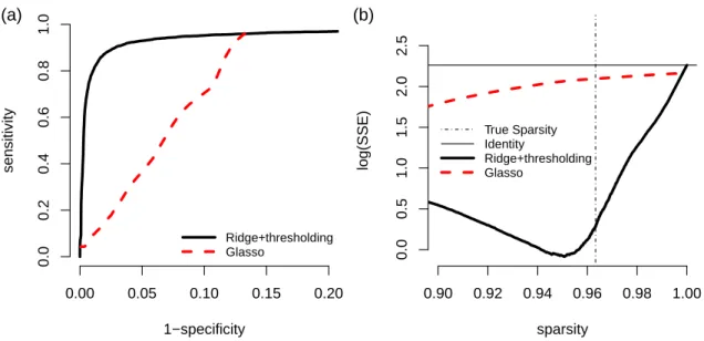
3.2 QQ-plots for p-values calculated using theoretical null distribution (black) or null distribution estimated by central matching method (green) against the expected uniform distribution on [0,1]. (a) p = 100 and n = 1000, (b) p= 100 andn = 110. The dotted lines are the 90% confidence limits of the expected values. . . 25 3.3 The ROC curve and SSE curve for n = 100, p = 50, and |E| = 45.

(a) ROC curve: 1-specificity versus sensitivity. (b) SSE curve: sparsity versus log(SSE). The horizontal black line is log(SSE) values when ap×p

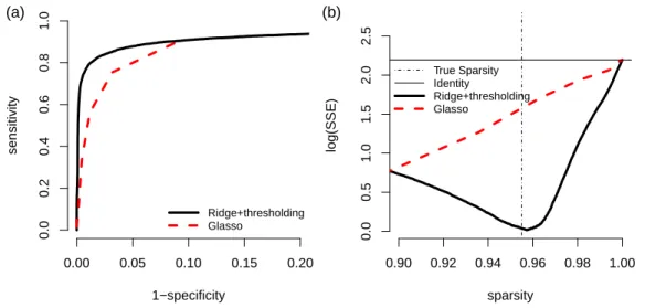
identity matrix is used and the vertical black line indicates the sparsity of the true network. . . 26 3.4 ROC curve and SSE curve for n = 100, p= 50, and |E|= 55. (a) ROC

curve: 1-specificity versus sensitivity. (b) SSE curve: sparsity versus log(SSE). The horizontal black line is log(SSE) values when a p × p

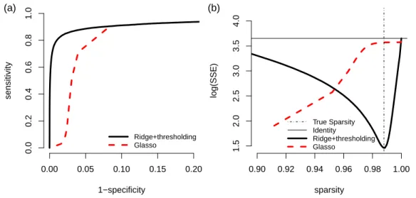
identity matrix is used and the vertical black line indicates the sparsity of the true network. . . 29 3.7 The ROC curve and SSE curve for n = 100, p = 200, and |E| = 160.

(a) ROC curve: 1-specificity versus sensitivity. (b) SSE curve: sparsity versus log(SSE). The horizontal black line is log(SSE) values when ap×p

identity matrix is used and the vertical black line indicates the sparsity of the true network. . . 30

(11)

3.8 ROC curve and SSE curve for n = 100, p = 200, and |E| = 200. (a) ROC curve: 1-specificity versus sensitivity. (b) SSE curve: sparsity versus log(SSE). The horizontal black line is log(SSE) values when a

p× p identity matrix is used and the vertical black line indicates the sparsity of the true network. . . 31 3.9 ROC curve and SSE curve for n = 100, p = 200, and |E| = 220. (a)

ROC curve: 1-specificity versus sensitivity. (b) SSE curve: sparsity versus log(SSE). The horizontal black line is log(SSE) values when a

p× p identity matrix is used and the vertical black line indicates the sparsity of the true network. . . 32 3.10 ROC curve and SSE curve for n = 100, p = 200, and |E| = 240. (a)

ROC curve: 1-specificity versus sensitivity. (b) SSE curve: sparsity versus log(SSE). The horizontal black line is log(SSE) values when a

p× p identity matrix is used and the vertical black line indicates the sparsity of the true network. . . 33 3.11 Comparing our method (Ridge+thresholding) with Glasso in terms

par-tial correlation graph estimation by ROC curves, while the underlying true connections are defined as gene pairs belonging the the same cluster and their proteins having protein-protein interaction. . . 34 4.1 Four DAGs where X and Z are not connected in the skeleton, but are

connected in the corresponding GGMs. . . 61 4.2 Histograms of the degree ν. (a) ER model with p= 1000 andpE = 2/p.

(b) BA model with p = 1000 and e = 1 and the log₁₀ scale density of log₁₀ν in its subplot. . . 62 4.3 Histograms of the degree ν under BA model with p = 1000 and e = 2

and the log₁₀ scale density of log₁₀ν in its subplot. . . 63 4.4 Performance of ER model (p= 11, n= 100, pE = 0.2). The upper panels

(12)

4.5 Performance of ER model (p = 100, n = 30, pE = 0.02). The upper panels are box plots (in log₁₀ scale) of true positive rate (TPR) (a), false positive rate (FPR) (b) and hamming distance (HD) (c) from 100 replications at α = 0.01. The lower panels are average true positive rate (d), false positive rate (e), and Hamming distance (f) from 100 replications when the tuning parameter α is changed from 0 to 0.1 (the grey vertical line are at α = 0.01). ROC curves are shown in panel (g). 65 4.6 Performance of ER model (p = 100, n = 30, pE = 0.03). The upper

panels are box plots (in log₁₀ scale) of true positive rate (TPR) (a), false positive rate (FPR) (b) and hamming distance (HD) (c) from 100 replications at α = 0.01. The lower panels are average true positive rate (d), false positive rate (e), and Hamming distance (f) from 100 replications when the tuning parameter α is changed from 0 to 0.1 (the grey vertical line are at α = 0.01). ROC curves are shown in panel (g). 66 4.7 Performance of ER model (p = 100, n = 30, pE = 0.04). The upper

panels are box plots (in log₁₀ scale) of true positive rate (TPR) (a), false positive rate (FPR) (b) and hamming distance (HD) (c) from 100 replications at α = 0.01. The lower panels are average true positive rate (d), false positive rate (e), and Hamming distance (f) from 100 replications when the tuning parameter α is changed from 0 to 0.1 (the grey vertical line are at α = 0.01). ROC curves are shown in panel (g). 69

(13)

4.10 Performance of ER model (p = 1000, n = 300, pE = 0.005). The upper panels are box plots (in log₁₀ scale) of true positive rate (TPR) (a), false positive rate (FPR) (b) and hamming distance (HD) (c) from 100 replications at α = 0.01. The lower panels are average true positive rate (d), false positive rate (e), and Hamming distance (f) from 100 replications when the tuning parameter α is changed from 0 to 0.1 (the grey vertical line are at α = 0.01). ROC curves are shown in panel (g). 70 4.11 Performance of ER model (p = 1000, n = 300, pE = 0.01). The upper

panels are box plots (in log₁₀ scale) of true positive rate (TPR) (a), false positive rate (FPR) (b) and hamming distance (HD) (c) from 100 replications at α = 0.01. The lower panels are average true positive rate (d), false positive rate (e), and Hamming distance (f) from 100 replications when the tuning parameter α is changed from 0 to 0.1 (the grey vertical line are at α = 0.01). ROC curves are shown in panel (g). 71 4.12 Performance of BA model (p=11,n=100,e=1). The upper panels are

box plots (in log₁₀ scale) of true positive rate (TPR) (a), false positive rate (FPR) (b) and hamming distance (HD) (c) from 100 replications at α = 0.01. The lower panels are average true positive rate (d), false positive rate (e), and Hamming distance (f) from 100 replications when the tuning parameter α is changed from 0 to 0.1 (the grey vertical line are at α= 0.01). ROC curves are shown in panel (g). . . 72 4.13 Performance of BA model (p=11,n=100,e=2). The upper panels are

(14)

4.15 Performance of BA model (p=100,n=30,e=2). The upper panels are box plots (in log₁₀ scale) of true positive rate (TPR) (a), false positive rate (FPR) (b) and hamming distance (HD) (c) from 100 replications at α = 0.01. The lower panels are average true positive rate (d), false positive rate (e), and Hamming distance (f) from 100 replications when the tuning parameter α is changed from 0 to 0.1 (the grey vertical line are at α= 0.01). ROC curves are shown in panel (g). . . 75 4.16 Performance of BA model (p=1000,n=300,e=1). The upper panels are

box plots (in log₁₀ scale) of true positive rate (TPR) (a), false positive rate (FPR) (b) and hamming distance (HD) (c) from 100 replications at α = 0.01. The lower panels are average true positive rate (d), false positive rate (e), and Hamming distance (f) from 100 replications when the tuning parameter α is changed from 0 to 0.1 (the grey vertical line are at α= 0.01). ROC curves are shown in panel (g). . . 77 4.18 (a) The distribution of standardized gene expression of all the genes

on all conditions (grey filled boxes) and standardized gene expression when a gene is knock down/knock out (black line boxes). (b) The den-sity of log₁₀ interventional effects. (c) The estimated causal effects from PC and PenPC algorithms, where regions R1-R4 are separated by hori-zontal/vertical lines at 0.8. (d) The distribution of log₁₀ interventional effects according to regions in (c). . . 78 4.19 Performance of causal effects prediction. (a) The ROC (receiver

operat-ing characteristic) curves of the PC and PenPCalgorithms, assuming the top m=10% of interventional effects are true positives. (b) The proce-dure (a) is repeated for m from 1 to 50 and the partial area under the ROC curve (pAUC) is plotted versus m values. . . 79 4.20 The distribution of ”expression change upon perturbation” for all knock

down/knock out genes (light grey) and those producing top 1% of the interventional effects . . . 80

(15)

4.21 (a) Edge occurrence (indicated by dark blue) in the estimated GGMs for 50 random permutations of variable orders, as well as the original order (shown as the first permutation). The variable pairs along the x-axis are ordered by their frequencies of being connected (by length 1 chain) across 51 permutations (from 51 to 1) and the variable pairs that are not connected in any permutation are excluded. (b) The density curve of the total number of edges in the estimated GGMs from 51 different variable orders (black line) and the number of edges in the GGM with the original order (red point). (c) The density curve of instability values for unstable variable pairs . . . 81 4.22 (a) Edge occurrence (indicated by dark blue) in the estimated skeletons

with α = 0.01 for 50 random permutations of variable orders, as well as the original order (shown as the first permutation). Here the step 2 of the PenPC algorithm is performed from the same GGM, which is estimated using the original ordering. The variable pairs along the x -axis are ordered by the frequencies of being connected (by length 1 chain) across 51 permutations (from 51 to 1) and the variable pairs that are not connected in any permutation are excluded. (b) The density curve of total number of edges in the estimated skeletons from 51 different variable orders (black line) and the number of edges in the skeletons with the original order (red point). (c) The density curve of instability values for unstable variable pairs. . . 82 4.23 Order-independent PenPC algorithm . . . 83 4.24 Estimation performance of order independent PenPC versus PC-stable

algorithm for different values of α and sample size n in the ER model with p = 1000 and pE = 0.002. The results are average from 100 ran-domly generated graphs. (a) Number of edges of skeleton estimates. (b) Hamming distance. (c) True discovery rate. (d) Structural Hamming distance. . . 84 4.25 Estimation performance of order independent PenPC versus PC-stable

(16)

5.2 Performances of the estimated skeleton from PC-stable algorithm (p=1000, n=300, pm = 0.3). Among 100 replications, 37 PDAGs (v-structures) were not extendable to a DAG. (a) Number of edges. (b) Number of true positives. (c) Number of false negatives. (d) Number of true negatives. (e) Number of false positives. (f) Hamming Distance. . . 104 5.3 Performances of CPDAG, directions when only eQTLs are used to

calcu-late likelihoods, QDG,siDAGfor q=100, 500, 800 and 1000 when p=1000, n=300, pm = 0.3 andpE = 0.002. Among true positive undirected edges in the skeleton estimates (a) number of undirected edges. (b) number of correct direction (c) number of incorrect directions. (d) Distance. . . 105 5.4 (a) Distribution of neighborhood sizes after the pre-screening procedure.

(b) Distribution of degree during PC-algorithm . . . 106 5.5 A scatter plot of the number of vertices versus the number of edges in

each module . . . 107 5.6 DAG estimation around gene ERBB2, where light blue edges are

un-directed edges. . . 108 5.7 DAG estimation around gene ESR1, where light blue edges are

un-directed edges. . . 109 5.8 DAG estimation around gene FGFR2, where light blue edges are

un-directed edges. . . 110

(17)

Chapter 1

Introduction

The relation of a set of random variables can be studied by graphical models, where the vertices represent the variables and edges capture the relations among the variables [Lauritzen, 1996]. A particular class of graphs, the directed acyclic graphs (DAGs) (also known as Bayesian Network) have been well studied for its importance in causal inference [Pearl, 2009]. In a DAG, all the edges are directed, and the direction of an edge implies a direct causal relation. There is no loop in a DAG, which is necessary to study causal relation [Spirtes et al., 2000]. Many methods have been developed to estimate DAGs from observational or interventional data, however, it remains a challenging problem in high dimensional setting where the number of variables can be larger or much larger than the sample size. The problem of DAG estimation in high-dimensional setting is the main focus of this dissertation.

(18)

to estimating the skeleton of a DAG. Given a CPDAG, we can use the intervention calculus method developed by Maathuis et al. [2009] to infer causal effects.

We first focus on estimating partial correlation matrix which describes correlations between variables given all the remaining variables. Under multivariate Gaussian as-sumption, zero partial correlation implies independence of two variables given all the other variables. A partial correlation graph can be constructed by connecting variables with non-zero partial correlations. Suppose a DAG can model the relation of a set of variables which follow a multivariate Gaussian distribution. Then the partial corre-lation graph of these variables is closely related to the underlying DAG because the former can be considered as a moral graph, which is obtained by connecting two par-ents sharing a common child in the DAG and replacing all directed edges by undirected edges. Under the multivariate Gaussian assumption, we propose a method to estimate the skeleton of a DAG by estimating the corresponding sparse partial correlation matrix in the first step and applying a series of partial correlation testings in the second step. Finally, we consider to use external data of “surrogate experiments” to orient the DAG skeleton Bareinboim and Pearl [2012]. In such surrogate experiments, interventions are applied on an additional set of variables that are directed causes of the variables of interest.

The remaining part of the dissertation is organized as follows. Chapter 2 includes some definitions and notations for DAGs. In Chapter 3, we propose an estimation method of sparse partial correlation matrix using ridge regression followed by thresh-olding by hypothesis testing. In Chapter 4, we estimate the skeletons of high dimen-sional DAGs by a two-step algorithm called PenPC. Finally in Chapter 5, we develop a method to orient the edges in a DAG skeleton using interventional data in surrogate experiments.

(19)

Chapter 2

Preliminaries on Directed Acyclic Graphs (DAGs)

2.1 Assumptions

A directed graph denoted by G is a pair (V, E), where V ={1, . . . p} is a finite set of vertices andE, the set of edges, is a subset of (V ×V)\ {(a, a)|a ∈V}. The edge set

E includes ordered pairs of distinct vertices and thus E includes no loops. A path of length n from i toj is a sequence i=i0 → i1 → · · · →in =j of distinct vertices such that (il−1, il)∈ E for l = 1, ..., n. Given this path, il−1 is a parent of il, il is achild of

il−1,i0, i1, ..., il−1 are ancestors of il, and il+1, ..., in are descendants of il. The graph G is called directed acyclic graph (DAG) if it contains no directed cyclic paths. Thus in a DAG, there is no path initiated from vertex i reaches i itself. The adjacency set of vertices ofj, denoted by adj(j,G), are the vertices that are connected toj by an edge of any directionality. Achain of lengthn fromitoj is a sequence i=i0, i1,· · · , in=j of distinct vertices such thatil−1 →il oril →il−1 forl = 1, ..., n.

Consider a DAG G whose vertices correspond to random variables X1, . . . , Xp and assume that

X = (X1, . . . , Xp)T ∈Rp ∼PX with density fX. (2.1)

(20)

recursive factorization

f(x1, . . . , xp) = p

Y

i=1

f(xi|xpa_i), (2.2)

where pa_i is defined by the set of parents of a vertex i ∈ V in G. The factorization naturally implies acyclic restriction of the graph structure. EquivalentlyPX is Markov to G if every variable is conditionally independent of its non-descendants given its parents.

The faithfulness assumption requires stronger relationship between distributionPX and DAGG than the Markov property.

Definition 1. LetPX be Markov toG. <G, PX >satisfies the faithfulness condtiontion

if and only if every conditional independence relation true in PX is entailed by the

Markov property applied to G [Spirtes et al., 2000].

This means that if a distribution PX is faithful to DAGG, all conditional indepen-dences can be read off from the DAG G using d-separation in the following definition 2.

Definition 2. (d-separation). A vertex set S block a chain p if either (i) p contains at least one arrow-emitting vertex that is in S, or (ii) p contains at least one collision vertex that is outside S and no descendant of the collision vertex belongs to S. If S

blocks all the chains from X to Y, it is said to “d-separate X and Y” [Pearl, 2009].

The faithfulness assumption allows no extra conditional independence relations in the distribution PX other than those which can be read from the DAG G using the d-separation. The more detailed description can be found in the literature [Robins et al., 2003]. DenotePX(G) as all distributions that are Markov toG. IfG represents the data generating machanism for PX, then PX is Markov to G, in other words PX ∈ PX(G). Given PX ∈PX(G), let T(PX) represent all independence relationships for variable X under PX. We say that PX is faithful toG if T(PX) = ∩Q∈PX(G)T(Q).

(21)

Not all the distributions can be faithfully represented by a DAG. If we assume that

X = (X1, ..., Xp)T ∈ _Rp _{follow multivariate normal distribution, the non-faithful ones} form a Lebesgue null set [Meek, 1995b] among all the multivariate normal distributions associated withG.

2.2 Partial correlation graph as a moral graph of DAG

Consider an undirected graph C = (V, F), where V = {1, . . . p} is a finite set of vertices corresponding to random variables X = (X1, . . . Xp)T with an unknown covariance matrixΣandF is a subset of (V ×V)\ {(a, a)|a∈V} including unordered pairs of distinct vertices. The distributionPX ofX is said tofactorize according to the undirected graphC if the joint density fX satisfies

fX(x1, . . . , xp) =

Y

C∈C

fC(xC), (2.3)

whereC is the set of cliques inC and fC is the joint density of variables XC ={Xi|i∈

C ⊆ V} [Lauritzen, 1996]. The undirected graph which satisfies the factorization property has Markov property: for any pair of vertices (i, j), (i, j) ∈ F if and only if Xi and Xj are conditionally independent given all the remaining variables {Xk|k ∈

V \ {i, j}}. The graph satisfying this Markov property is called independence graph. The partial correlation graph under the Gaussian assumption is independence graph and is often called Gaussian graphical model (GGM). The covariance selection problem Dempster [1972] is equivalent to the estimation ofC because conditional independence relations implied by the factorization on C can be identified by the zero structure of the inverse covariance matrix denoted by Ωunder the normality assumption.

For a DAG G = (V, E) we can define its moral graph for the same set of vertices

(22)

and subsequently deleting directions on all edges [Lauritzen, 1996]. Assuming the factorizations both on G and C, it is easily seen that the moral graph of G is C by lemma 3.21 of [Lauritzen, 1996].

2.3 Identifiability of DAG

A DAGGis not identifiable from the distributionPX which is assumed to be Markov to G because several different DAG’s may determine the same PX. In other words, because several different DAGs may determine the same set of conditional independence restrictions among a given set of random variables, the collection of all possible DAGs for these variables naturally coalesces into one or more classes of Markov equivalent

DAGs, where all DAGs within a Markov class determine the same statistical model (the same factorization) [Andersson et al., 1997]. The following theorem well characterizes the Markov equivalence class.

Theorem 1. Two DAG’s are Markov equivalent if and only if they have the same skeleton and the same v-structure [Andersson et al., 1997].

The skeleton of a DAG G is obtained by replacing all directed edges to undirected edges: the skeleton is denoted byGu _{= (}_{V, E}u_{) where (}_{i, j}₎_∈_Eu _⇔₍_{i, j}₎_∈_E _{or (}_{j, i}₎_∈

E. The v-structure is an ordered triple of vertices (i, j, k) such that G contains the directed edges (i, k) ∈ E and (j, k) ∈ E and i and j are not adjacent in G: in this v-structure, the co-parents i and j share a common child k which is called a collision

vertex. The distribution PX is faithful to G if and only if (i) for any vertex pair (i, j) in V, (i, j) ∈ Eu _{if and only if} _i _and _j _{are dependent conditional on every subset in}

V \ {i, j} and (ii) in a v-structure i → k ← j, i and j are marginally independent or conditionally independent given the parents of iand j, butiand j are dependent with each other given every set that containk (a collision vertex) or its descendants but not

i orj.

(23)

(24)

Chapter 3

Partial Correlation Matrix Estimation Using Ridge Penalty Followed by Hypothesis Testing

3.1 Introduction

The expression of multiple genes can be studied through a network perspective, where the set of genes of interest are vertices and the relations among the genes are undirected/directed edges. The gene coexpression network analysis is a popular ap-proach to dissect gene expression regulation patterns and to detect functionally related genes [Stuart et al., 2003; de Jong et al., 2012]. In this chapter we study the (undi-rected) co-expression network of a group of genes constructed through their partial correlation matrix, where the partial correlation of two genes is a measure of the linear relationship of these two genes’ expression conditioning on the expression of all the other genes.

We consider a p-dimensional random vector (i.e., the expression of p genes) X = (X1, ..., Xp)T ∈ Rp with an unknown covariance matrix Σ. Assuming that the co-variance matrix Σ is positive definite, let Ω = [Ωab]p×p = Σ−1 be the inverse of the covariance matrix. Ωis also called concentration matrix or precision matrix. The par-tial correlations can be obtained by the off diagonal elements of the negative definite matrix

(25)

where thescaleis an operator defined for a square matrix. Letdiag(A) be a diagonal matrix constructed by the diagonal elements ofA, then

scale(A) =diag(A)−1/2Adiag(A)−1/2.

The derivation of equation (3.1) is presented in the Appendix I. The zero structure of the partial correlation matrix ofprandom variables can be represented by an undirected graph

G= (Γ,E),

where Γ = {1,· · · , p} is the set of vertices and E is a set of edges in Γ ×Γ such that any edge between vertices a and b belongs to E if and only if ρab 6= 0, i.e, the two random variables Xa and Xb are conditionally correlated given all the remaining variablesXΓ\{a,b} ={Xk:k ∈Γ\ {a, b}}. We refer to such an undirected graphGas a

partial correlation graph. Under multivariate Gaussian distribution assumption forX, the zero off-diagonal entries of ΩorR occur if and only if the corresponding variables are conditionally independent given the remaining variables.

(26)

ridge estimates is desirable because it leads to parsimonious and more interpretable partial correlation matrix estimate. Such thresholding often further reduces estimation error, and provides a logical connection between estimation and testing.

Next we briefly review the existing works for estimating concentration matrix or partial correlation matrix and related statistical inference. Assume X = (X1, ..., Xp)T follows multivariate Gaussian distribution, denoted by N(µ,Σ). Suppose there are n

independent samples ofX. LetX be thep×n centered data matrix. Assumingµ=0, the log-likelihood of concentration matrix Ω is proportional to

l(Ω) = log|Ω| −tr(SΩ), (3.2)

where tr(·) is trace of a square matrix and S = XXT/n is the sample covariance matrix. Whenn ≥p, Sis positive definite with probability 1 and S−1 is the maximum likelihood estimate (MLE) of Ω [Lauritzen, 1996]. However, this approach fails when

p > n, and may perform poorly unless n is much larger than p. Therefore MLE with certain constraints or penalized MLE are often used for high dimensional problems when p is lager or much larger than n. Examples include covariance selection from positive definite matrices [Dempster, 1972] or iterative partial maximization based on deviance tests [Speed and Kiiveri, 1986]. More general linear restrictions on edges are enabled by colored graph models [Højsgaard and Lauritzen, 2008]. Recently, many penalized MLE ofΩhave been proposed for high dimensional problems [Yuan and Lin, 2007; Rothman et al., 2008; Banerjee et al., 2008; Friedman et al., 2008; Fan et al., 2009]. One of the most widely used methods is the graphic Lasso [Friedman et al., 2008], which maximizes the following penalized log likelihood:

l(Ω) = log|Ω| −tr(SΩ)−κX

a,b

|Ωab|, (3.3)

(27)

whereκ is a tuning parameter.

With a focus on determining the partial correlation graph, rather than precise es-timation of the partial correlation coefficients, Meinshausen and B¨uhlmann [2006] pro-posed a regression-based approach calledneighborhood selection. The neighborhood for each vertex was estimated by penalized regression of the corresponding variable versus the remaining variables. Banerjee et al. [2008]; Friedman et al. [2008] showed that estimating the penalized MLE (with L1 penalty) of Ω could be viewed as p-coupled

iterative versions of the pseparate neighborhood selections. More recent methodology developments related with neighborhood selection include Yuan [2010] and Zhou et al. [2011].

Statistical inference of partial correlation estimates is another topic related with our method development. Given a partial correlation estimate, denoted by ˆρ, one may test H0 : ρ = 0 against HA : ρ 6= 0 using a test statistic constructed by Fisher’s Z-transformation: ψ( ˆρ) = 0.5 log{(1 + ˆρ)/(1−ρˆ)}. Specifically, one may reject the null hypothesis at level α if (n−p−1)1/2|ψ( ˆρ)| >Φ−1(1−α/2) for standard normal c.d.f. Φ [Anderson, 2003]. However, this testing procedure assumes the sample size n

(28)

the 0-1 partial correlation graph to an arbitrary q ≤ p−2 order partial correlation graph.

The remaining parts of the chapter are organized as follows. We present our method in Section 3.2, demonstrate the effectiveness of our method by simulations and real data analysis in Section 3.3, and conclude this chapter by some discussions in Section 3.4.

3.2 Method

3.2.1 Estimation of partial correlation matrix using ridge penalty

We assume the p×n data matrix X has been centered so that S = XXT_/n _is

the sample covariance matrix. Then a straightforward estimate of (the off-diagonal elements of) a partial correlation matrix can be obtained from

ˆ

R=−scale(S−1₎_.

However, whenn < p, Sis not invertible. To solve the singularity problem of inverting a sample covariance matrix, we add a positive constant to the diagonal elements of the sample covariance matrix:

ˆ

R(λ) = −scale (S+λIp)−1

, (3.4)

whereλ≥0 andIp is ap×pidentity matrix. We callS+(λ) = (S+λIp)−1 as theridge inverse in the analogy to ridge regression [Hoerl and Kennard, 1970]. The modified sample covariance matrix S+λIp guarantees full rank for any λ > 0, and has been used as an initial covariance matrix estimate in the coordinate descent algorithms in Banerjee et al. [2008]; Friedman et al. [2008].

Next we show that as λ varies from 0 to ∞, ˆR(λ) varies from a scaled generalized

(29)

inverse to an identity matrix. Let X/√n =UDVT be a singular value decomposition with rank(X) = k ≤ min(n, p), where U and V are, respectively p×p and n× n

orthogonal matrices, D is p × n diagonal matrix with its first k nonzero diagonal elementsd1, . . . , dk and all other elements being zero. Since S+(λ) =U(D+λIp)−1UT, it is obvious that

scale S+(λ)→scale(S−) as λ→0, (3.5)

whereS− is Moore-Penrose generalized (MPG) inverse of Sif k < p [Schott, 2005]. By the invariance of thescale operator under scalar product,

scale S+(λ)

=scale λS+(λ)

→Ip asλ→ ∞. (3.6)

Since the estimates of regression coefficients using MPG inverse is minimumL2 solution

(proposition 1 of Lv and Fan [2009]),S+(λ) goes tok rank ridge inverse whenλgoes to 0 by (3.5). From (3.6) the partial correlation matrix shrinks toward the identity matrix asλ goes to infinity.

S+₍_λ_{) can also be understood as the inverse of a shrinkage estimate of the covariance}

matrix [Sch¨afer et al., 2005] since we can rewriteS+₍_λ_{) as}

cS+(λ) = ((1−λ0)S+λ0Ip)

−1

, (3.7)

whereλ0 =λ/(1 +λ) and c= (1 +λ).

We choose the tuning parameterλin the ridge inverse by its equivalence relationship with pseparate ridge regressions. Given λ, for anya ∈Γ, the ridge coefficients are

ˆ

βa(λ) = arg min β∈Rp−1

1

n(Xa−X−aβ) T

(Xa−X−aβ) +λβTβ,

(30)

matrix for n measurements of the remainingp−1 variables X−a. Given the following decomposition of the sample covariance matrixS with respect to variables (Xa, X−a),

S=



 

Sa,a Sa,−a S−a,a S−a,−a





,

ˆ

βa₍_λ_{) has a closed-form solution}

ˆ

βa(λ) = (S−a,−a+λIp−1)−1S−a,a.

Now we show that estimating the off-diagonal elements of ˆR(λ) is the same as estimat-ing regression coefficients usestimat-ing p separate ridge regressions. Let

W=S+(λ) =



 

Sa,a+λ Sa,−a S−a,a S−a,−a+λIp−1



 

−1

=



 

Wa,a Wa,−a W−a,a W−a,−a





.

From the inverse formula for block matrices,

W−a,a =−Wa,a(S−a,−a+λIp−1)−1S−a,a =−Wa,aβˆa(λ).

Therefore the estimation of partial correlation matrix is equivalent to estimating the regression coefficients p separate ridge regressions. To choose the tuning parameter λ, we minimize 10-fold cross validation estimates of the total prediction errors of the p

ridge regressions.

3.2.2 Thresholding

We propose a hypothesis testing approach to threshold the off-diagonal elements of the ridge estimates ˆR(λ) = [ ˆρλ

ab]p×p. We use Fisher’s Z-transformation of partial

(31)

correlations as our test statistics, denoted by {ψ( ˆρλ_ab) : a ∈ Γ, b ∈ Γ, and a 6= b}. By taking advantage of the sparsity of the high dimensional partial correlation matrix, we estimate the null distribution of our test statistics from data using Efron’s central matching method. Although our testing approach can apply to a variety of partial correlation estimates, we develop it here for the ridge inverse estimate.

Following Efron [2004], we assume the observed test statistics follow a mixture

distribution

f(ψ) = (1−η)f0(ψ) +ηfa(ψ), (3.8)

where the null distribution f0(ψ) is a normal distribution N(µ0, σ2₀), the alternative distributionfa(ψ) is left un-specified, andηis the proportion of the observations arising from the non-null distribution. We also assume that a large proportion of the observed

ψ values are from the null distribution, i.e. η≈ 0. This assumption reflects the belief that the partial correlation matrix is sparse. Then the central part of the marginal distribution of ψ is mostly occupied by the observations from the null distribution and only the tail areas of the marginal distribution are affected by the small proportion of non-null observations. Therefore using Efron’s central matching method, we can estimate the null distribution (i.e., estimate µ0 and σ0) by matching the marginal distribution and the null distribution at the center part of the distributions. Specifically, assuming f(ψ) = f0(ψ) around ψ = 0 gives

logf(ψ) = −1 2

ψ−µ₀

σ0

2

+C (3.9)

for a constant C.

We estimate the density f(ψ) using polynomial poisson regression. The range of the p(p−1)/2 observed ψ values is partitioned into K equal intervals with interval

(32)

independently distributed following Poisson distributions with mean νk’s. We fit a q degree polynomial Poisson regression on νk,

log(νk) = log f(xk)/c

= q

X

j=1

θj(xk)j, (3.10)

for k = 1, ..., K and a normalizing constant c making the marginal density f(ψ) inte-grated to 1. The estimates of {θj : j = 1, . . . , q} are used to estimate log ˆf(ψ)/c

=

Pq

j=1θˆjψ

j_{. Then using equation (3.9), we can obtain the estimates of} _µ

0 and σ0:

ˆ

µ0 = arg max n

ˆ

f(ψ)o, σˆ0 =

− d

2

dψ2 log ˆf(ψ)

−1₂

ψ=ˆµ0

. (3.11)

The degree of polynomial regression,q, is a nuisance parameter. Based on the sparsity assumption that most p-values arise from the null, we choose theq so that the p-values are most uniformly distributed. The empirical distribution function of the p-values, {π(_abq)|a6=b∈Γ} given q, is

Fq(π) = 2

p(p−1)

X

a,b∈Γ,a6=b

I(π(_abq) ≤π). (3.12)

We suggest to estimateq by

ˆ

q= arg min q

h

sup

0<π<1

|Fq(π)−F0(π)| i

, (3.13)

whereF0(π) is uniform distribution between 0 and 1, andDq = sup0<π<1|Fq(π)−F0(π)|

is a distance measure used in Kolmogorov-Smirnov statistic. Figure 3.1 displays the average and one standard deviation of Dq values over 100 simulation data sets for

p = 500, n = 30 and η = 0 or η = 0.0003, which corresponds to 38 non-zero partial correlations. Adding 38 nonzero partial correlations to the null needs 3 or 4 higher

(33)

polynomial order on average to estimate the null distribution.

3.2.3 Re-estimation of partial correlation coefficients

Given the zero structure estimated in the previous step, we re-estimate the partial correlation coefficients at the non-zero entries of the partial correlation matrix. Suppose that the covariance matrixΣand the concentration matrixΩare partitioned according to random variables (Xa, X−a) and the blocks are denoted byΣa,a,Σ−a,a,Σa,−a,Σ−a,−a and Ωa,a, Ω−a,a,Ωa,−a,Ω−a,−a. Consider the best linear predictor of Xa byX−Taβa for any a ∈ Γ. Let a = Xa−X−Taβa. It is easy to show that βa = Σ

−1

−a,−aΣ−a,a and Var(Xa −X−Taβa) = Var(a) = Σa,a − Σa,−aΣ−−1a,−aΣ−a,a. From inverse formula for block matrix andΩ=Σ−1_,

Ωa,a= (Var(a))−1, Ω−a,a =−(Var(a))−1βa. (3.14)

From ˆE(λ, α) estimated in the thresholding step, we know all the variables adjacent to

a ∈Γ, denoted by ˆnea. Based on the sparsity assumption, we assume |neaˆ |< n, then we can have the following refined estimates of the concentration matrix:

˜

Ωaa = (n− |neaˆ |)/kXa−Xneaˆ βâ,neaˆ k22, Ω˜−aa =−Ωãaβâ,neaˆ , (3.15)

where ˆβa,neaˆ ₌ _X ˆ neaXTneaˆ

−

Xneaˆ Xa, Xneaˆ is |neˆa| ×n submatrix of X corresponding to ˆnea, and (·)− is the k = min(n,|neˆa|) rank ridge inverse using MPG inverse. Since this solution is not symmetric in general, we set the final estimates of the off-diagonal elements of Ωas

ˆ

Ωa,b= ˆΩb,a =sign( ˆβba,neaˆ )

q

˜

(34)

and the partial correlation coefficients estimates from −scale( ˆΩ).

3.3 Results

3.3.1 Simulation I

We first use a simple simulation to demonstrate that the p-values calculated using central matching method follow the expected uniform distribution under null, while the p-values calculated using asymptotic distribution can lead to inflated type I error. We simulated data from multivariate Gaussian distribution N(0,Ip×p) with p = 100 and n = 1000 or 110. All pairwise partial correlations were calculated by inverting the sample correlation matrix, and then the test statistics were calculated by Fisher’s Z transformation of the partial correlations. The p-values of the test statistics were calculated using theoretical null distribution N(0,1/n−p−1), and the empirical null distribution estimated by central matching method. As shown in the qq-plots of Fig-ure 3.2, whenp= 100 andn= 1000, p-values calculated using either the theoretical null distribution or the empirical null distribution followed the expected uniform distribu-tion. However when the sample size was decreased ton = 110, the p-values calculated from the empirical null distribution were still uniformly distributed but the p-values calculated from the theoretical null distribution were severely inflated.

3.3.2 Simulation II

We consider random networks where both the network structure and the partial correlation coefficients are random. The only restriction is that the partial correlation matrix is diagonally dominant, so that R is a strictly negative definite matrix. The simulation datasets were generated following similar approach of Sch¨afer and Strimmer [2005]. We simulated ap×ndata matrixXcomposed ofnindependent random samples frompdimensional multivariate Gaussian distributionNp(0,Σ), whereΣis determined

(35)

by a simulated concentration matrix Ω. We initialized Ω by a p×p matrix with all elements being 0’s. Givenη, the proportion of non-null edges among all thep(p−1)/2 edges, we randomly selected 100η% of the off-diagonal elements ofΩand filled in values from uniform distribution on [-1,1]. To ensure that Ωis a positive definite matrix, the diagonal elements of Ωwere filled by column-wise sums of absolute values plus a small constant. FinallyΣ was calculated by scale(Ω−1_).

Let |E| be the number of edges in setE. Our simulation settings are 1. p= 50, n = 100, and |E|= 45,55,65,75

2. p= 200, n = 100, and|E|= 160,200,220,240.

We evaluated the accuracy of partial correlation graph using ROC curve, and the accuracy of partial correlation coefficient estimates using sum squared error (SSE). Given the set of vertices Γ={1,2, ..., p}, The SSE was calculated as

L(R,R) =ˆ X a6=b∈Γ

( ˆρab−ρab)2, (3.17)

where ˆR = [ ˆρab]p×p was the estimates of R. For either the ROC curve of the SSE value, the mean values calculated from 100 replicates of each simulation setting were reported.

We compared our method with one of the most widely used method for partial correlation matrix estimation, the Graphical Lasso (Glasso) [Friedman et al., 2008]. For our method, we used 10-fold cross-validation to choose the value of ridge parameter

(36)

method and across different values of the tuning parameter κ of the Glasso. In the ROC curves for both high and low dimension cases, our method has uniformly better sensitivity and and specificity than the Glasso in estimating the network structure. The SSE curves show that our method attains lower SSE value than the Glasso around the true sparsity level.

3.3.3 Application

We applied our method to estimate the partial correlation graph of the expres-sion of 6178 genes from yeast cell cycle data [Spellman et al., 1998]. The gene ex-pression data were downloaded fromhttp://genome-www.stanford.edu/cellcycle/ data/rawdata/. After removing the samples with more than 20% missing values, 75

samples remained for further analysis. We imputed the remaining missing values of the expression data using nearest neighbor averaging. Then the expression data of each sample were normalized by quantile normalization. In this analysis we did not account for the time-dependent nature of the data and treated the expression of each gene across 75 samples as independent observations.

Denote the observed gene expression data as a matrix X of dimension 6178×75. Each gene is a variable, and thusΓis{1, ...,6178}. We first grouped the 6178 genes into

h clusters. Let Ci be the genes belonging to the i-th cluster, then

Ph

i=1|Ci| = 6178. We separately constructed the partial correlation graph within each cluster. The graph of ith cluster is denoted by GCi = (Ci, ECi) for i = 1, . . . , h. We assumed the genes

from different clusters were independent, so that the edge setE of the whole graph was estimated by ˆE=Sh

i=1EˆCi. Specifically, we clustered the 6178 genes using hierarchical

clustering with Ward’s minimum variance method and the distance between two genes

aand b was defined as 1− |ˆρab|∅| where ˆρab|∅ denoted marginal Pearson correlation. We

chose the number of clusters to be 25 based on thegap statistic [Tibshirani et al., 2001].

(37)

Cluster sizes varied from 32 to 1370, with 25 percentile, median, and 75 percentile being 139, 194, and 254, respectively. Among all the 19,080,753 gene pairs of the 6178 genes, 1,556,154 belonged to the same cluster, and hence could be connected based on the partial correlation graph estimates.

We compared the performance of our method with the Glasso [Friedman et al., 2008]. We chose the tuning parameter κ of Glasso based on the extended Bayesian information criterion (BIC) [Foygel and Drton, 2010]:

BICγ(κ) =−log|Ω(ˆ κ)|+tr( ˆΩ(κ)S) + 1

n|

ˆ

E(κ)|logn+ 4

n|

ˆ

E(κ)|γlogp, (3.18)

where ˆΩ(κ) was the estimate of the inverse covariance matrix using Glasso with tuning parameter κ, ˆE(κ) was the edge set obtained from ˆΩ(κ), and γ ∈ [0,1] is a tuning parameter of the extended BIC. If γ = 0, the classical BIC used in Yuan and Lin [2007] was recovered. Given a fixedγ value, we applied Glasso with tuning parameter selected by the extended BIC (3.18) to construct the partial correlation graphs for all 25 clusters. An exception is that for two clusters with low dimension such thatp < n/2, we always used the classical BIC by setting γ = 0. Different choices of γ led to the different model selection results.

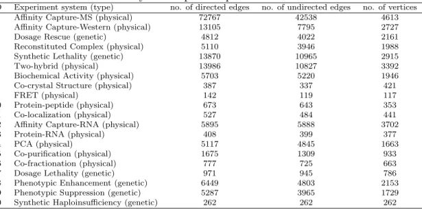
The estimates of partial correlation graphs were evaluated by comparing the edge set ˆE with yeast protein-protein interaction database at http://thebiogrid.org/ download.php. Table 3.1 displays the number of directed edges, the number of

(38)

our method and Glasso by ROC curves. The ROC curve of our method was generated across different p-value cutoffsαand the ROC curve of the Glasso was generated across different γ values in the extended BIC. Our method had uniformly higher sensitivity and specificity than the Glasso (Figure 3.11) to predict protein-protein interactions in the database.

3.4 Discussion

We have described a new framework for estimation and statistical inference of par-tial correlation matrix. Both simulation and real data analysis have demonstrated the effectiveness of our method. For real data analysis where p is much larger than n, we cluster the genes and then estimate partial correlation matrix within each cluster. This is based on an reasonable assumption that the partial correlation matrix of gene expression has a block diagonal structure. We used the hierarchical clustering to group genes. There are many other clustering method available Monti et al. [2003]; Zhang et al. [2005], though a careful study of which clustering method can better identify the block diagonal structure is beyond the scope of this chapter. Our method does not require multivariate Gaussian distribution assumption. However, without this assump-tion, partial correlation being zero may not imply the two variables are independent with each other.

(39)

3.5 Tables and figures

Table 3.1: Summary of the protein-protein interaction database

ID Experiment system (type) no. of directed edges no. of undirected edges no. of vertices 1 Affinity Capture-MS (physical) 72767 42538 4613 2 Affinity Capture-Western (physical) 13105 7795 2727

3 Dosage Rescue (genetic) 4812 4022 2161

4 Reconstituted Complex (physical) 5110 3946 1988 5 Synthetic Lethality (genetic) 13870 10965 2915

6 Two-hybrid (physical) 13986 10827 3392

7 Biochemical Activity (physical) 5703 5220 1946 8 Co-crystal Structure (physical) 387 337 421

9 FRET (physical) 142 119 117

10 Protein-peptide (physical) 673 643 353

11 Co-localization (physical) 527 484 441

12 Affinity Capture-RNA (physical) 5895 5888 3702

13 Protein-RNA (physical) 408 399 377

14 PCA (physical) 5117 4845 1663

15 Co-purification (physical) 1675 1309 933

16 Co-fractionation (physical) 777 725 663

17 Dosage Lethality (genetic) 971 945 786

(40)

● ●

● ● ● ●

2 4 6 8 10 12 14

0.01

0.03

0.05

0.07

q

Dq

● η=0

η=0.0003

Figure 3.1: The degree of polynomials q versus the average Kolmogorov-Smirnov dis-tanceDq with one standard deviation from 100 replications for (p= 500, n = 30, η= 0) and (p= 500, n = 30, η= 0.0003) using ridge inverse with λ= 1e−08.

(41)

(42)

0.00 0.05 0.10 0.15 0.20

0.0

0.2

0.4

0.6

0.8

1.0

1−specificity

sensitivity

Ridge+thresholding Glasso

(a)

0.90 0.92 0.94 0.96 0.98 1.00

0.0

0.5

1.0

1.5

2.0

2.5

sparsity

lo

g

(SSE)

True Sparsity Identity

(b)

Figure 3.3: The ROC curve and SSE curve for n = 100, p = 50, and |E| = 45. (a) ROC curve: 1-specificity versus sensitivity. (b) SSE curve: sparsity versus log(SSE). The horizontal black line is log(SSE) values when a p×p identity matrix is used and the vertical black line indicates the sparsity of the true network.

(43)

0.00 0.05 0.10 0.15 0.20

0.0

0.2

0.4

0.6

0.8

1.0

1−specificity

sensitivity

(a)

0.90 0.92 0.94 0.96 0.98 1.00

0.0

0.5

1.0

1.5

2.0

2.5

sparsity

lo

g

(SSE)

(b)

(44)

0.00 0.05 0.10 0.15 0.20

0.0

0.2

0.4

0.6

0.8

1.0

1−specificity

sensitivity

(a)

0.90 0.92 0.94 0.96 0.98 1.00

0.5

1.0

1.5

2.0

2.5

sparsity

lo

g

(SSE)

(b)

Figure 3.5: ROC curve and SSE curve for n = 100, p = 50, and |E| = 65. (a) ROC curve: 1-specificity versus sensitivity. (b) SSE curve: sparsity versus log(SSE). The horizontal black line is log(SSE) values when a p×p identity matrix is used and the vertical black line indicates the sparsity of the true network.

(45)

0.00 0.05 0.10 0.15 0.20

0.0

0.2

0.4

0.6

0.8

1.0

1−specificity

sensitivity

(a)

0.90 0.92 0.94 0.96 0.98 1.00

0.5

1.0

1.5

2.0

2.5

sparsity

lo

g

(SSE)

(b)

(46)

0.00 0.05 0.10 0.15 0.20

0.0

0.2

0.4

0.6

0.8

1.0

1−specificity

sensitivity

(a)

0.90 0.92 0.94 0.96 0.98 1.00

2.5

3.0

3.5

4.0

sparsity

lo

g

(SSE)

(b)

Figure 3.7: The ROC curve and SSE curve for n = 100, p = 200, and |E| = 160. (a) ROC curve: 1-specificity versus sensitivity. (b) SSE curve: sparsity versus log(SSE). The horizontal black line is log(SSE) values when a p×p identity matrix is used and the vertical black line indicates the sparsity of the true network.

(47)

0.00 0.05 0.10 0.15 0.20

0.0

0.2

0.4

0.6

0.8

1.0

1−specificity

sensitivity

(a)

0.90 0.92 0.94 0.96 0.98 1.00

1.5

2.0

2.5

3.0

3.5

4.0

sparsity

lo

g

(SSE)

(b)

(48)

0.00 0.05 0.10 0.15 0.20

0.0

0.2

0.4

0.6

0.8

1.0

1−specificity

sensitivity

(a)

0.90 0.92 0.94 0.96 0.98 1.00

1.5

2.0

2.5

3.0

3.5

4.0

sparsity

lo

g

(SSE)

(b)

Figure 3.9: ROC curve and SSE curve for n = 100, p= 200, and |E|= 220. (a) ROC curve: 1-specificity versus sensitivity. (b) SSE curve: sparsity versus log(SSE). The horizontal black line is log(SSE) values when a p×p identity matrix is used and the vertical black line indicates the sparsity of the true network.

(49)

0.00 0.05 0.10 0.15 0.20

0.0

0.2

0.4

0.6

0.8

1.0

1−specificity

sensitivity

(a)

0.90 0.92 0.94 0.96 0.98 1.00

1.5

2.0

2.5

3.0

3.5

4.0

sparsity

lo

g

(SSE)

(b)

(50)

0 20 40 60 80 100

0.0

0.5

1.0

1.5

# of edges not in the database (thousand)

# of edges in the database (thousand)

Ridge+thresholding glasso

Figure 3.11: Comparing our method (Ridge+thresholding) with Glasso in terms partial correlation graph estimation by ROC curves, while the underlying true connections are defined as gene pairs belonging the the same cluster and their proteins having protein-protein interaction.

(51)

Chapter 4

PenPC: A Two-step Approach to Estimate the Skeletons of High Dimensional Directed Acyclic Graphs

4.1 Introduction

The relation of a set of random variables can be studied by graphical models, where vertices represent the variables and edges capture the relations among the variables [Lauritzen, 1996]. A particular class of graphs, the directed acyclic graphs (DAGs) (also known as Bayesian Network) have been well studied for its importance in causal inference [Pearl, 2009]. For example, in genomic studies, DAGs have been employed to study gene expression regulation [Friedman, 2004; Sachs et al., 2005; Zhang et al., 2010; Bonn et al., 2012]. In a DAG, all the edges are directed, and the direction of an edge implies a direct causal relation. There is no loop in a DAG, which is necessary to study causal relation [Spirtes et al., 2000]. When we remove the directions of all the edges in a DAG, the resulting undirected graph is the skeleton of the DAG.

(52)

2010]. Several methods have been developed to estimate DAGs or their skeletons [Heck-erman et al., 1995; Spirtes et al., 2000; Chickering, 2003; Kalisch and B¨uhlmann, 2007], however most of them are only computationally feasible when the number of variables

p is smaller or comparable to sample size n, with the exception of the PC-algorithm (named after its authors, Peter and Clark). Kalisch and B¨uhlmann [2007] proved that under some regularity conditions, the PC-algorithm consistently estimates the skeleton of sparse DAG for high-dimensional problems where p = O(nr) for r > 0. In this chapter, we proposed a new method named PenPC to address this challenging skele-ton estimation problem. We proved the estimation consistency of PenPCunder weaker regularity conditions for high dimensional settings of p = O(nr_{) or} _p ₌ _O_(exp{_na_}). As verified by both simulation and real data analysis, PenPC provides more accurate estimates of the skeletons than the PC-algorithm.

The remaining parts of this chapter is organized as follows. In section 4.2, we give a brief review of Gaussian Graphical Models (GGMs), DAGs, and the conceptual advantage of our PenPC algorithm. Details of the PenPC algorithm is introduced in section 4.3 and its theoretical properties are presented in section 4.4. In section 4.5, we compare the performances of the PenPC and the PC algorithms by simulations. In section 4.6, we further evaluate thePenPC and the PC algorithms in real data analysis where causal effects estimated from observational data can be assessed by interventional data. In section 4.7, we observe order-dependency of PenPC algorithm and introduce order-independentPenPC. Finally, we conclude in section 4.8.

4.2 Review of Gaussian Graphical Models and DAGs

4.2.1 Gaussian Graphical Models (GGMs)

We consider a p-dimensional random vector X = (X1, ..., Xp)T ∈ Rp following a multivariate normal distribution Np(µ,Σ) with unknown mean values µ and a p×p

(53)

non-singular covariance matrixΣ. LetΩ= [ωij]p×p =Σ−1be the concentration matrix or precision matrix. Under multivariate normal assumption, ωij = 0 if and only if Xi is independent with Xj given all other p−2 variables. Therefore Ω is also known as partial covariance matrix. Letn be the sample size and denote then×pobserved data matrix byX= (x1, ...,xp). Recently, a significant amount of works have been devoted to the estimation of Σ [Bickel and Levina, 2008; Levina et al., 2008; Rothman et al., 2008, 2009; Lam and Fan, 2009; Cai and Liu, 2011] orΩ[Yuan and Lin, 2007; Rothman et al., 2008; Banerjee et al., 2008; Friedman et al., 2008; Fan et al., 2009; Yuan, 2010] from the observed data matrixXin high dimensional problems wherep is much larger than n, see [Pourahmadi, 2011] for a recent review.

In this chapter, we are particularly interested in the identification of the non-zero entries of Ω, known as the covariance selection problem [Dempster, 1972]. It has been recognized that covariance selection and the estimation of concentration matrix are different problems [Meinshausen and B¨uhlmann, 2006; Yuan, 2010]. For example, the neighborhood selection method [Meinshausen and B¨uhlmann, 2006], which separately selects the neighbors of each vertex by a penalized regression with p−1 covariates, consistently estimates the nonzero elements of Ω, but only provides an approximate, instead of exact Penalized Maximum Likelihood Estimate (PMLE) of Ω [Friedman et al., 2008].

Assuming that the variables of interestX = (X1, ..., Xp)Tfollow multivariate normal distribution, this covariance selection problem is equivalent to constructing a Gaussian Graphic Model (GGM). A GGM of X is an undirected graph C = (V, F) where V

contains p vertices correspond to X1, ..., Xp, and F contains all the undirected edges

(54)

the skeleton of a DAG because of v-structures. In a v-structure X →W ← Z, X and

Z are marginally independent or conditionally independent given the parents of X and

Z, but given every set that contain W (a collision vertex) but not X or Z, X and Z

are dependent with each other. For example, consider a sprinkler which is scheduled to spray at certain time every day. Either rain or the sprinkler may lead to the wet grass. Given the event that the grass is wet, there is a negative correlation between the event “sprinkler being on” and the event of rain [Pearl, 2009]. Other examples include the DAGs shown in Figure 4.1(a-d), whereX and Z are not connected in skeleton, but they are connected in the corresponding Gaussian Graphic Models. Instances of the covariance and concentration matrices of the GGM in Figure 4.1(a) are shown in the Appendix II. The true network skeleton that there is no edge betweenX and Z can be identified by examining marginal correlations or conditional correlations. For example,

X ⊥Z in Figure 4.1(a),X ⊥Z|Y in Figure 4.1(b),X ⊥Z|(Y, U) in Figure 4.1(c), and

X ⊥Z|Y in Figure 4.1(d).

When the p variables are ordered by the underlying DAG’s topology, such as

Xi ⊥ {Xi+1, ..., Xp} | {X1, ..., Xi−1} for i = 2, ..., p−1, the problem of skeleton

es-timation is greatly simplified because a regression of Xi versus X1, ..., Xi−1 can be

used to identify the true skeleton. Such a multiple regression won’t be confused by v-structures because a common child of vertexes Xi and Xj will never appear as a co-variate of the regression models usingXi orXj as the response variable. In fact, Shojaie and Michailidis [2010] have shown that when the p variables are ordered by network topology, a neighborhood selection using the predecessors of each variable yields the exact PMLE of the concentration matrix rather than an approximation. However, in high-dimensional real data analysis problems, the topology order is rarely available. Throughout this chapter, we assume such an topology order is unknown.

(55)

4.2.2 Directed Acyclic Graph (DAGs)

A DAG of random variables X1, ..., Xp is a directed graph with no cycle (or loop). Specifically, a DAG can be denoted byG= (V, E), whereV containspvertices 1,2, ...., p

that correspond to X1, ..., Xp, andE contains all the directed edges. In a DAG, apath of length n from i to j is a sequence i = i0 → i1 → · · · → in = j of distinct vertices such that (il−1, il)∈E forl = 1, ..., n. Given this path,il−1 is aparent ofil,il is achild ofil−1, i0, i1, ..., il−1 are ancestors of il, andil+1, ..., in are descendants of il. In a DAG, there is no path initiated from vertex i reaches i itself. This restriction of no cycle is necessary for causal inference. The adjacency set of vertices ofj, denoted byadj(j,G), are the vertices that are connected toj by an edge of any directionality.

Achain of lengthnfromitoj is a sequencei=i0, i1,· · · , in =j of distinct vertices such that il−1 →il or il → il−1 for l = 1, ..., n. A DAG can graphically represent the

conditional independence relationships amongpvariables by the followingd-separation

concept. A vertex set S block a chain p if either (i) p contains at least one arrow-emitting vertex that is in S, or (ii) p contains at least one collision vertex that is outsideS and has no descendant of the collision vertex in S. If S blocks all the chains fromX to Y, it is said to “d-separate X and Y” [Pearl, 2009].

Not all the distributions can be faithfully represented by a DAG. A probability dis-tributionP isfaithful with respect to a DAGG if the conditional independence ofP is equivalent to d-separation inG. In this chapter, we assume thatX = (X1, ..., Xp)T ∈_Rp follow multivariate normal distribution. Among all the multivariate normal distribu-tions associated with G, the non-faithful ones form a Lebesgue null set [Meek, 1995b]. In the following discussions, we assume the faithfulness of the distributions.

(56)

distribution and they form an equivalence class, which can be described by a com-pleted partially directed acyclic graph (CPDAG) [Chickering, 2002]. Identification of v-structures (hence a CPDAG), after skeleton estimation, only requires application of a set of deterministic rules, which is described in the Appendix II. Given a CPDAG, we can use the intervention calculus method developed by [Maathuis et al., 2009] to infer causal effects.

4.2.3 Constraint based approaches

In this section we will review constraint based methods to estimate the Markov equivalence class of a DAG. Under faithfulness assumption, the Inductive Causation (IC) algorithm aims at estimating the CPDAG of a DAG and the algorithm consists of three steps: (1) estimation of the skeleton by a set of conditional independence tests, (2) v-structure identification, and (3) completion of the PDAG obtained from (1) and (2) [Pearl, 2009]. The resulting graph is CPDAG which represents the Markov equivalence class of a DAGG. After estimating skeletons using conditional independence tests, the steps (2) and (3) proceed by applying several deterministic rules described in [Pearl, 2009; Spirtes et al., 2000; Meek, 1995a; Chickering, 2002; Dor and Tarsi, 1992]. The estimation accuracy mostly depends on the first step, the sekeleton estimation.

Spirtes et al. [2000] describes various algorithms to estimate the skeleton. SGS algo-rithm starts from a complete undirected graph where any pair of vertices are connected then thins the graph by removing the edgesi−j such that Yi and Yj are conditionally independent given any subset in V \ {i, j}. PC algorithm thins the correlation graph by removing edges with first order conditional independence relations, thins again with second order conditional independence relations, and so on. The SGS algorithm relies on higher order conditional independence testings even for sparse graphs while for the PC algorithm, the set of variables conditioned on requires only be a subset of the set of

(57)

variables adjacent to one or the other variables tested. Subsequently, IG algorithm first estimate the undirected independence graph which is GGM under Gaussian assump-tion, then SGS algorithm is applied in each clique to exclude the false connections. As a variation of the IG algorithm, Spirtes et al. [2000] also suggested to apply PC algorithm in the second step.

In a high dimensional and sparse setting, Kalisch and B¨uhlmann [2007] proved uniform consistency of PC-algorithm when p = O(na) for a > 0. Specifically, each test of conditional independence has certain probability of making a mistake, and they showed that under some regularity and sparsity conditions, the summation of these mistaken probabilities goes to 0. Using stability selection, Stekhoven et al. [2012] shows the improvement of IDA method in Maathuis et al. [2009] which provides estimated lower bounds of total causal effects based on the estimated CPDAG from PC-algotirhm. Colombo and Maathuis [2012] improved PC-algorithm by solving the order dependency from which the resulting skeleton depends on the variable ordering of the input data. It is calledPC-stable algorithm.