Tree Edit Distance Cannot be Computed in Strongly Subcubic
Time (unless APSP can)
Karl Bringmann∗ Paweł Gawrychowski† Shay Mozes‡ Oren Weimann†
Abstract
The edit distance between two rooted ordered trees withnnodes labeled from an alphabetΣ is the minimum cost of transforming one tree into the other by a sequence of elementary oper-ations consisting of deleting and relabeling existing nodes, as well as inserting new nodes. Tree edit distance is a well known generalization of string edit distance. The fastest known algorithm for tree edit distance runs in cubicO(n3)time and is based on a similar dynamic programming
solution as string edit distance. In this paper we show that a truly subcubic O(n3−ε) time
algorithm for tree edit distance is unlikely: For|Σ|= Ω(n), a truly subcubic algorithm for tree edit distance implies a truly subcubic algorithm for the all pairs shortest paths problem. For |Σ|=O(1), a truly subcubic algorithm for tree edit distance implies anO(nk−ε)algorithm for
finding a maximum weightk-clique.
Thus, while in terms of upper bounds string edit distance and tree edit distance are highly related, in terms of lower bounds string edit distance exhibits the hardness of the strong ex-ponential time hypothesis [Backurs, Indyk STOC’15] whereas tree edit distance exhibits the hardness of all pairs shortest paths. Our result provides a matching conditional lower bound for one of the last remaining classic dynamic programming problems.
1
Introduction
Tree edit distance is the most common similarity measure between labelled trees. Algorithms for computing the tree edit distance are being used in a multitude of applications in various do-mains including computational biology [24,37,52,58], structured text and data processing (e.g., XML) [30,31,36], programming languages and compilation [38], computer vision [22,43], character recognition [49], automatic grading [14], answer extraction [65], and the list goes on and on.
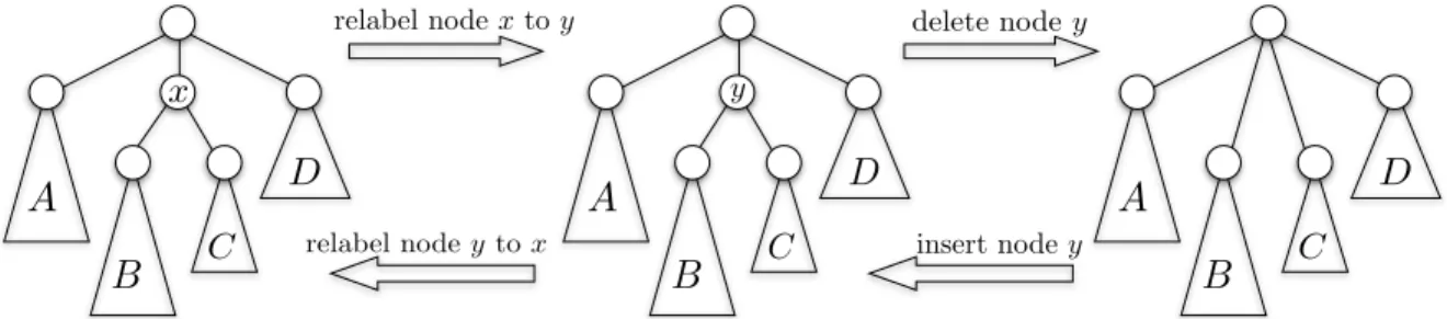
LetF andGbe two rooted trees with a left-to-right order among siblings and where each vertex is assigned a label from an alphabetΣ. The edit distance betweenF andGis the minimum cost of transforming F into Gby a sequence of elementary operations (at most one operation per node): changing the label of a node v, deleting a node v and setting the children of v as the children of
v’s parent (in the place of v in the left-to-right order), and inserting a node v (the complement of delete1). See Figure 1. The cost of these elementary operations is given by two functions: c
del(a)
is the cost of deleting or inserting a vertex with label a, and cmatch(a, b) is the cost of changing the
label of a vertex fromato b. ∗
Max Planck Institute for Informatics, Saarland Informatics Campus
†
University of Haifa. Partially supported by the Israel Science Foundation grant 794/13.
‡
IDC Herzliya. Partially supported by the Israel Science Foundation grant 794/13.
1Since a deletion inF is equivalent to an insertion inGand vice versa, we can focus on finding the minimum cost
of a sequence of just deletions and relabelings in both trees that transformF andGinto isomorphic trees.
x
A
B
C DA
B
C DA
B
C D relabel nodextoy y delete nodey insert nodey relabel nodey toxFigure 1: The three editing operations on a tree with vertex labels.
The Tree Edit Distance (TED) problem was introduced by Tai in the late 70’s [55] as a gener-alization of the well known string edit distance problem [57]. Since then it was extensively studied. Tai gave anO(n6)-time algorithm for TED which was subsequently improved toO(n4) in the late 80’s [53], then to O(n3logn) in the late 90’s [41], and finally to O(n3) in 2007 [34]. Many other algorithms have been developed for TED, see the popular survey of Bille [24] (this survey alone has more than 600 citations) and the books of Apostolico and Galil [16] and Valiente [56]. For example, Pawlik and Augsten [48] recently defined a class of dynamic programming algorithms that includes all the above algorithms for TED, and developed an algorithm whose performance on any input is not worse (and possibly better) than that of any of the existing algorithms. Other attempts achieved better running time by restricting the edit operations or the scoring schemes [31,51,54,66], or by resorting to approximation [12,17]. However, in the worst case no algorithm currently beats
Ω(n3) (not even by a logarithmic factor).
Due to their importance in practice, many of the algorithms described above, as well as additional heuristics and optimizations were studied experimentally [39,48]. Solving tree edit distance in truly subcubic O(n3−ε) time is arguably one of the main open problems in pattern matching, and the
most important one in tree pattern matching.
The fact that, despite the significant body of work on this problem, no truly subcubic time algorithm has been found, leads to the following natural conjecture that no such algorithm exists.
Conjecture 1. For any >0Tree Edit Distance on two n-node trees cannot be solved inO(n3−) time.
In the same paper proving theO(n3)upper bound for TED [34], Demaine et al. prove that their algorithm is optimal within a certain class of dynamic programming algorithms for TED. However, proving Conjecture1 seems to be beyond our current lower bound techniques.
A recent development in theoretical computer science suggests a more fine-grained classification of problems in P. This is done by showing lower bounds conditioned on the conjectured hardness of certain archetypal problems such as All Pairs Shortest Paths (APSP), 3-SUM, k-Clique, and Satisfiability, i.e., the Strong Exponential Time Hypothesis (SETH).
The APSP Conjecture. Given a directed or undirected graph withnvertices and integer edge weights, many classical algorithms for APSP (such as Dijkstra or Floyd-Warshall) run inO(n3)time. The fastest to date is the recent algorithm of Williams [60] that runs faster thanO(n3/logCn)time
for all constants C. Nevertheless, no truly subcubic O(n3−ε) time algorithm for APSP is known.
Conjecture 2 (APSP). For any ε >0 there exists c >0, such that All Pairs Shortest Paths on n
node graphs with edge weights in {1, . . . , nc} cannot be solved inO(n3−ε) time.
The (Weighted) k-Clique Conjecture. The fundamental k-Clique problem asks whether a given undirected unweighted graph on n nodes and O(n2) edges contains a clique on k nodes. This is the parameterized version of the famously NP-hard Max-Clique [40]. k-Clique is amongst the most well-studied problems in theoretical computer science, and it is the canonical intractable (W[1]-complete) problem in parameterized complexity. A naive algorithm solvesk-Clique inO(nk)
time. A fasterO(nωk/3)-time algorithm (whereω <2.373is the exponent of matrix multiplication) can be achieved via a reduction to Boolean matrix multiplication on matrices of size nk/3 ×nk/3 if k is divisible by 3 [47]2. Any improvement to this bound immediately implies a faster algorithm for MAX-CUT [59,64]. It is a longstanding open question whether improvements to this bound are possible [46,63]. The k-Clique conjecture asserts that for no k≥3 and ε >0 the problem has an
O(nωk/3−ε) time algorithm, or an O(nk−ε) algorithm avoiding fast matrix multiplication, and has
been used e.g. in [3,28].
We work with a conjecture on a weighted version of k-Clique. In the Max-Weight k-Clique
problem, the edges have integral weights and we seek thek-clique of maximum total weight. When the edge weights are small, one can obtain an O˜(nk−ε) time algorithm [13,47]. However, when the
weights are larger thannk, the trivialO(nk) algorithm is the best known (ignoring no(k) improve-ments). This gives rise to the following conjecture, which has been used e.g. in [10,18,21].
Conjecture 3 (Max-Weightk-Clique). For any ε >0 there exists a constant c >0, such that for anyk≥3 Max-Weightk-Clique onn-node graphs with edge weights in{1, . . . , nck}cannot be solved in O(nk(1−ε)) time.
In 2014, with the burst of the conditional lower bound paradigm, Abboud [1] highlighted seven main open problems in the field: The first two were to prove quadraticn2−o(1)lower bounds forString
Edit Distance and Longest Common Subsequence, which were soon resolved in STOC’15 [19] and FOCS’15 [4,29] conditional on SETH. The third problem was to show a cubicn3−o(1)lower bound for
RNA-Folding. Surprisingly, in FOCS’16 [27] it was shown that RNA-Folding can actually be solved in truly subcubic time, thus ruling out the possibility of such a lower bound. The remaining four problems remain open. In fact, two of them, showing a cubic lower bound forGraph Diameter and anndk/2e−o(1) lower bound fork-SUM, have actually been used as hardness conjectures themselves, e.g., in SODA’15 [6] and ICALP’13 [8]. Until the present work, no progress has been made on the last problem posed by Abboud: A cubic lower bound for Tree Edit Distance. In the absence of progress on either upper bounds or conditional lower bounds for TED, one might think that Conjecture 1 is yet another fragment in the current landscape of fine grained complexity, and is unrelated to other common conjectures.
1.1 Our Results
In this paper we resolve the complexity of tree edit distance by showing a tight connection between edit distance of trees and all pairs shortest paths of graphs. We prove that Conjecture 2 implies Conjecture 1, and that Conjecture3 implies Conjecture1, even for constant alphabet.
2
Theorem 1. A truly subcubic algorithm for tree edit distance on alphabet size|Σ|= Ω(n) implies a truly subcubic algorithm for APSP. A truly subcubic algorithm for tree edit distance on sufficiently large alphabet size|Σ|=O(1) implies an O(nk(1−ε)) algorithm for Max-Weight k-Clique.
Note that the known upper bounds for string edit distance and tree edit distance are highly related. The O(n2) algorithm for strings and theO(n3) algorithm for trees (and forests) are both based on a similar recursive solution: The recursive subproblems in strings (forests) are obtained by either deleting, inserting, or matching the rightmost or leftmost character (root). In strings, it is best to always consider the rightmost character. The recursive subproblems are then prefixes and the overall running time isO(n2). In trees however, sticking with the rightmost (or leftmost) root may result in an O(n4) running time. The specific way in which the recursion switches between leftmost and rightmost roots is exactly what enables theO(n3)solution. It is interesting that while the upper bounds for both problems are so similar, the lower bounds string edit distance exhibits the hardness of the SETH while tree edit distance exhibits the hardness of APSP.
While a considerable share of the recent conditional lower bounds is on string pattern matching problems [3,4,7,10,15,19,20,28,29,32,45], the only conditional lower bound for a tree pattern matching problem is the recent SODA’16 quadratic lower bound for exact pattern matching [2] (the problem of deciding whether one tree is a subtree of another). We solve the main remaining open problem in tree pattern matching, and one of the last remaining classic dynamic program-ming problems. Indeed, apart from the problems discussed above, for most of the classic dynamic programming problems a conditional lower bound or an improved algorithm have been found re-cently. This includes the Fréchet distance [25], bitonic TSP [33], context-free grammar parsing [3], maximum weight rectangle [18], and pseudopolynomial time algorithms for subset sum [26]. Tree edit distance was one of the few classic dynamic programming problems that so far resisted this approach. Two notable remaining dynamic programming problems without matching bounds are the optimal binary search tree problem (O(n2)) [44] and knapsack (pseudopolynomialO(nW)) [23].
1.2 Our Reductions
APSP to TED. In order to prove APSP-hardness, by [61] it suffices to show a reduction from the negative triangle detection problem, where we are given ann-node graphG with edge weights
w(., .) and want to decide whether there are i, j, k with w(i, j) +w(j, k) +w(i, k) < 0. Our first result is a reduction from negative triangle detection to tree edit distance, which produces trees of size O(n) over an alphabet of size O(n). This yields the matching conditional lower bound of
O(n3−ε).
Our reduction constructs trees that are of a very special form: Both trees consist of a single path (called spine) of lengthO(n) with a single leaf pending from every node (see Figure 2). Such instances already have been identified as difficult for a restricted class of algorithms based on a specific dynamic programming approach [34]. In our setting we cannot assume anything about the algorithm, and hence need a deeper insight on the structure of any valid sequence of edit operations (see Figure 2and Lemma 1). Using this structural understanding, we then show that it is possible to carefully construct a cost function so that any optimal solution must obey a certain structure (Figure 3). Namely, for some i, j, k we match the two leaves in depth k, we match the right spine node in depthk to the left leaf in depth i(which encodesw(i, k)), we match the left spine node in depth k to the right leaf in depth j (which encodes w(j, k)), and we match as many spine nodes above depthiand j as possible (which together encodew(i, j) by a telescoping sum).
Constant alphabet size. The drawback of the above reduction is the large alphabet size |Σ|, as essentially each node needs its own alphabet symbol. There are two major difficulties to improving this to constant alphabet size.
First, the instances identified as hard by the above reduction (and by Demaine et al. [34] for a restricted class of algorithms) are no longer hard for small alphabet! Indeed, in Section 4 we give anO(n2|Σ|2logn)algorithm for these instances, which is truly subcubic for constant alphabet size. This algorithm is the first to break the barrier by Demaine et al. for such trees, and we believe it is of independent interest. Regarding lower bounds, this algorithm shows that for a reduction with constant alphabet size our trees necessarily need to be more complicated, making it much harder to reason about the structure of a valid edit sequence. We will construct new hard instances by taking the previous ones and attaching small subtrees to all nodes.
The second difficulty is that, since the input size of TED is O˜(n+|Σ|2), a reduction from negative triangle detection to TED with constant alphabet size would need to considerably compress theΩ(n2) input size of negative triangle detection. It is a well-known open problem whether such compressing reductions exist. To circumvent this barrier, we assume the stronger Max-Weight
k-Clique Conjecture, where the input sizeO˜(n2)is very small compared to the running timeO(nk).
Max-Weightk-Clique to TED. Given an instance of Max-Weightk-Clique on ann-node graph
G and weights bounded by nO(k) we construct a TED instance on trees of size O(nk/3+2) over an alphabet of size O(k). One can verify that an O(n3−ε) algorithm for TED now implies an
O(nk(1−ε/6)) algorithm for Max-Weight k-Clique, for any sufficiently large k=k(ε).
We roughly follow the reduction from negative triangle detection; now each spine node corre-sponds to ak/3-clique inG. To cope with the small alphabet, we simulate the previous matching costs with small gadgets. In particular, to each spine node, corresponding to somek/3-cliqueU, we add a small subtreeT(U)of sizeO(n2)such that the edit distance betweenT(U)andT(U0)encodes the total weight of edges between U and U0. This raises two issues. First, we need to represent a weight w∈ {0, . . . , nO(k)} by trees over an alphabet of sizeO(k) (that is, constant). This is solved by writing w in base n as PO(k)
i=0 αini and constructing αi nodes of type i, such that the cost of
matching two type inodes is ni. A second issue is that we need the small subtreeT(U) to interact
with every other small subtree T(U0). So, in a sense,T(U) needs to “prepare” for any possibleU0, and yet its size needs to be small. We achieve this by creating in T(U0), for every node u inG, a separate component responsible for counting the total weight of all edges between u and all nodes inU0. Then, in T(U) we have a separate component for every node u∈ U, and make sure that it is necessarily matched to the appropriate component in T(U0).
The final and most intricate component of our reduction is to enforce that in any optimal solution we have some control on which small subtrees can be matched to which. A similar issue was present in the negative triangle reduction, when we require control over which spine nodes above depth i
are matched to which spine nodes above depthj. This is handled in the negative triangle reduction by assigning a different matching cost depending on the node’s depth. Now however, we cannot afford so many different costs. We overcome this with yet another gadget, called anI-gadget, that achieves roughly the same goal, but in a more “distributed” manner.
Both of our reductions are highly non-trivial and introduce a number of new tricks that could be useful for other problems on trees.
2
Reducing APSP to TED
We re-define the cost of matching two nodes to be the original cost minus the cost of deleting both nodes. Then, the goal of TED amounts to choosing a subset of red nodes in both trees, so that the subtrees defined by the red nodes are isomorphic (i.e., their left-right and ancestor-descendant relation is the same in both trees) and the total cost of matching the corresponding red nodes is minimized. See Figure2. We work with this formulation from now on.
fip+1 fi1 fip fip+2 fip+q+1 fip+q+2 gjp+q+2 gjp+q+1 gjp+2 gjp+1 gjp gj1
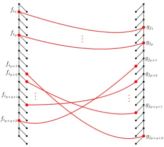
Figure 2: Macro structure of the hard instance for TED: A tree F composed of a single spine with leaves hanging to the right and a tree Gcomposed of a single spine with leaves hanging to the left.
It turns out that a hard instance for TED is given by two seemingly simple caterpillar trees. These two trees F and G, also called left and right, are shown in Figure2. Each tree consists of
spine nodes andleaf nodes. Ifuis a spine node then we denote byu0 the (unique) leaf node attached to u. For any such hard instance of TED, the red nodes in any matching have the structure given by Lemma1below. Informally, it states that starting from the top of the left tree and ordering the nodes by depth, the matching consists of (1) a prefix of a matching subsequence of spine nodes in both trees, (2) a suffix of a matching subsequence of leaf nodes that are in reverse order in the other tree, and (3) at most one final spine node in each of the trees matching a leaf node in the other tree that is located between the prefix part (1) and the suffix part (2).
Lemma 1. Let f1, f2, . . .and g1, g2, . . . denote the spine nodes ofF andG, respectively, ordered by
the depth. Then, for some p, q ≥0 and some i1 < i2· · · < ip < ip+1 <· · ·< ip+q+1 < ip+q+2 and
j1< j2· · ·< jp < jp+1<· · ·< jp+q+1< jp+q+2 the set of red nodes consists of:
(1) Spine nodesfi1, fi2, . . . , fip matched respectively to spine nodes gj1, gj2, . . . , gjp,
(2) Leaf nodesfi0p+2, fi0p+3, . . . , fi0p+q+1 matched respectively to leaf nodesg0jp+q+1, gj0p+q, . . . , gj0p+2 (note the reversed order),
(3) Optionally, a spine nodefip+q+2 matched to leaf node g
0
jp+1. Also optionally, a spine nodegjp+q+2 matched to a leaf node fi0p+1.
Proof. Consider the subtree defined by the red nodes. It has two isomorphic copies, one inF and one in G. Its nodes are all the red nodes. The children of node u are all red nodes v1, v2, . . . , vk
whose lowest red ancestor is u. The order is such that vi precedes vi+1 in a left-to-right preorder traversal ofF (or equivalently ofG). Letu be a red node with two or more childrenv1, v2, . . . , vk,
k ≥ 2. Observe that u must correspond to spine nodes in both F and G. Further observe that at most one vi can correspond to a spine node (otherwise, for two spine nodes one must be an
ancestor of the other). Consider any`∈ {1,2, . . . , k−1}. It is not hard to see that nodev`+1 must correspond to a leaf node inF and nodev` must correspond to a leaf node inG. This implies that
bothv` andv`+1 are leaves in the red subtree. Moreover,v1is the only node that may correspond to a spine node inF andvkis the only node that may correspond to a spine node inG. Consequently,
the red subtree has a particularly simple structure: it consists of nodes u1, u2, . . . , up such that for
every`= 1,2, . . . , p−1the only child of u` isu`+1, and nodes v1, v2, . . . , vk (for some k≥1) that
are all children ofup.
For every ` = 1,2, . . . , p, the node u` must correspond to a spine node fi` ∈ F and gj` ∈ G.
We immediately obtain (1) that i1 < i2 < . . . < ip and that j1 < j2 < . . . < jp. The nodes
v1, v2, . . . , vkare all children ofup in the subtree. It is possible that allvi are mapped to leaf nodes
f0 ip+2, f 0 ip+3, . . . , f 0 ip+q+1 and g 0 jp+2, g 0 jp+3, . . . , g 0
jp+q+1. In this case, they must be mapped in reverse
order since a left-to-right preorder traversal visits the leaves of G in order of their depth and in reverse-depth order in F. This implies (2) that ip ≤ ip+2 < . . . < ip+q+1 and jp ≤ jp+2 < . . . <
jp+q+1. Recall however that v1 may be mapped to a spine node fip+q+2 inF and a leaf node g
0
jp+1
inG. The requirement that ip+q+2 > ip+q+1 and thatjp+2 > jp+1 ≥jp follows from the fact that
these nodes correspond to a leftmost leaf in the subtree. For symmetric reasons,vkmay be matched
to a spine node gjp+q+2 ∈G for somejp+q+2 > jp+q+1 and ip+2 > ip+1 ≥ip. This implies(3) and
concludes the proof.
The above lemma characterizes the structure of a solution to what we call the hard instance of TED. We next show how to reduce the negative triangle detection problem to TED on the hard instance. Negative triangle detection is known to be subcubic equivalent to APSP [61]. Given a complete weightedn-node undirected graph, where w(i, j)denotes the weight of the edge(i, j), the problem asks whether there are i, j, k such that w(i, j) +w(j, k) +w(i, k) < 0. To solve negative triangle detection, we clearly only need to find i, j, k that minimizew(i, j) +w(j, k) +w(i, k). We will show how to construct, given such a graph, a hard instance of TED of size O(n), such that
mini,j,kw(i, j) +w(j, k) +w(i, k) can be extracted from the edit distance.
Lemma 2. Given a complete undirected n-node graph G with weights w(., .) in {1, . . . , nc}, we construct, in linear time in the output size, an instance of TED of size O(n) with alphabet size
|Σ|=O(n)such that the minimum weight of a triangle inGcan be extracted from the edit distance.
Consequently, an O(n3−) time algorithm for TED implies an O(n3−) algorithm for negative
triangle detection, and thus an O(n3−/3)algorithm for APSP by a reduction in [61].
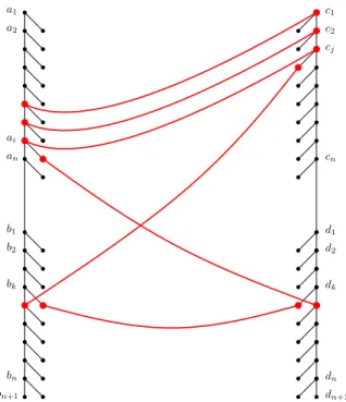
We create a hard instance of TED consisting of two trees F andGas in Figure 3. Every tree is divided into atop and abottom part. The spine nodes of these parts are denoted bya1, a2, . . . , an
for the top left part,b1, b2, . . . , bn+1 for the bottom left part,c1, c2, . . . , cnfor the top right part, and
d1, d2, . . . , dn+1 for the bottom right part. The labels of all nodes are distinct (hence the alphabet size |Σ| is Θ(n)). We set the cost cmatch(u, v) of matching two nodes u and v as described below, where M denotes a sufficiently large number to be specified later. Intuitively, our assignment of costs ensures that any valid solution to TED must match b0k to d0k, bk+1 to c0j, and dk+1 to a0i for
a1 a2 an b1 b2 bn c1 c2 cn d1 d2 dn ai cj bk dk bn+1 dn+1
Figure 3: A hard instance of TED constructed for a given instance of negative triangle detection. Appropriately chosen costs ensure that any optimal solution has a specific structure.
some i, j, k (as shown in Figure3). Furthermore, the optimal solution (i.e., of minimum cost) must choose i, j, k that minimize w(i, k) +w(k, j) +w(i, j). The costs are assigned as follows:
(1) cmatch(b 0 k, d 0 k) =−M2−2M ·kfor every k= 1,2, . . . , n. (2) cmatch(bk+1, c 0
j) =−M2+M·k+M·j+w(k, j) for everyk= 1,2, . . . , n andj= 1,2, . . . , n.
(3) cmatch(a0i, dk+1) =−M2+M·k+M·i+w(i, k) for everyi= 1,2, . . . , nand k= 1,2, . . . , n.
(4) cmatch(ai, cj) =−2M+w(i, j)−w(i−1, j−1)for every i= 2,3, . . . , n and j= 2,3, . . . , n.
(5) cmatch(ai, c1) =−M(i+ 1) +w(i,1)for every i= 1,2, . . . , n.
(6) cmatch(a1, cj) =−M(j+ 1) +w(1, j) for everyj = 1,2, . . . , n.
All the remaining costscmatch(u, v)are set to∞. The following theorem proves that these costs
imply the required structure on the optimal solution as described above. Intuitively, by choosing sufficiently largeM, because of the−M2 addend in(1),(2)and(3)we can ensure that any optimal solution matchesb0ktod0k,bk0+1to c0
j, anddk00+1 toa0
i, for somei, j, kandk0, k00≤k. Then, because
of the M·k in (2)and (3), in any optimal solution actually k= k0 = k00 and the total cost of all these matchings is w(k, j) +w(i, k). Finally, because of the−2M in(4), the −M(i+ 1) in(5), and the−M(j+ 1)in(6), in any optimal solutionai is matched tocj,ai−1 to cj−1,ai−2 tocj−2 and so on. The total cost of these matching is w(i, j) since thew(i, j)−w(i−1, j−1)terms in (4)form a telescoping sum.
Theorem 2. For sufficiently largeM, the total cost of an optimal matching in a hard instance with costs(1)-(6)is −3M2+ min
i,j,kw(i, k) +w(k, j) +w(i, j).
Proof. Consider i, j, k minimizing w(i, k) +w(k, j) +w(i, j). We assume without loss of generality thati≥j. It is easy to see that it is possible to choose the following matching (see Figure3):
1. b0 k to d0k with cost−M2−2M·k. 2. bk+1 to c0j with cost −M2+M ·k+M·j+w(k, j). 3. dk+1 to a0i with cost−M2+M·k+M ·i+w(i, k). 4. ai to cj,ai−1 to cj−1,ai−2 tocj−2, . . . , ai−j+2 to c2 with costs−2M+w(i, j)−w(i−1, j− 1),−2M+w(i−1, j−1)−w(i−2, j−2), . . . ,−2M +w(i−j+ 2,2)−w(i−j+ 1,1). 5. ai−j+1 to c1 with cost −M·(i−j+ 2) +w(i−j+ 1,1).
Summing up and telescoping, the total cost is−M2−2M·k−M2+M·k+M·j+w(k, j)−M2+M·k+
M·i+w(i, k)−2M·(j−1)+w(i, j)−M·(i−j+2)which is equal to−3M2+w(i, k)+w(k, j)+w(i, j). For the other direction, we need to prove that every solution has cost at least −3M2 +
mini,j,kw(i, k) +w(k, j) +w(i, j). We first observe that, by Lemma 1, a solution can match b0k
to d0k at most once for somek. Similarly, it can match bk0+1 to c0j at most once for somej and k0, and dk00+1 to a0
i at most once for some iand k00. Furthermore, for M large enough, either the cost
is larger than −3M2 or all three such pairs of nodes are matched for some k, i, j, and k0, k00 ≥k. Furthermore, if k0 > k and M is large enough then we can decrease k0 by one thus decreasing the total cost, and similarly ifk00 > k. It is enough to consider an optimal solution and hence we can assume thatk=k0 =k00.
Again by Lemma 1, the only possible additional matched pairs of nodes are a subsequence of spine nodesa1, . . . , aiandc1, . . . , cj. We show that an optimal solution matchesaiwithcj,ai−1with
cj−1, ..., ai−j+1 withc1. To this end, suppose thataxz is matched tocyz, for everyz= 1,2, . . . , L,
where1≤x1 < . . . < xL≤iand 1≤y1 < . . . < yL≤j. For every z this contributes, up to lower
order terms less thanM,−2M if xz, yz >1, or−M(yz+ 1)ifxz = 1, or −M(xz+ 1)if yz = 1. In
an optimal solution we have x1 = 1 or y1 = 1, as otherwise we can match a1 to c1 to decrease the total cost. First, assume that y1 = 1. Then, ifxz0+ 1< xz0+1 for some z0 ∈ {1, . . . , L} (where we definexL+1=i+ 1), we can increase allx1, x2, . . . , xz0 by 1 to decrease the total cost byM, up to lower order terms. SoxL=i, xL−1=i−1, . . . , x1=i−L+ 1. Now ifL < jthenx1>1(recall that we assumedi≥j) and alsoyz0+ 1< yz0+1 for somez0 ∈ {1, . . . , L}(again, we defineyL+1=j+ 1). This means that we can increase all y1, y2, . . . , yz0 by 1 and then additionally match ax1−1 withc1 to decrease the total cost byM, up to lower order terms. Second, if x1 = 1a symmetric argument applies. We obtain that indeed L= min(i, j) =j, andai−j+1 is matched toc1,ai−j+2 is matched toc2, ...,ai is matched tocj. Now, by the same calculations as in the previous paragraph, the total
cost is −3M2+w(i, k) +w(k, j) +w(i, j).
3
Reducing Max-Weight
k
-Clique to TED
The drawback of the reduction described in Section2is the large size of the alphabet. That is, given a complete weightedn-node undirected graph it creates two trees of sizeO(n) where labels of nodes are distinct, and therefore |Σ|= Θ(n). We would like to refine the reduction so that |Σ|= O(1).
However, as the input size of TED onn-node trees and alphabetΣwithO(logn)-bit integer weights is O˜(n+|Σ|2), such a reduction would need to compress the O˜(n2) input size of negative triangle detection considerably. To circumvent this barrier, we assume the stronger Max-Weight k-Clique Conjecture, where the input sizeO˜(n2) is very small compared to the running time boundO(nk). Lemma 3. Given a complete undirectedn-node graphGwith weights in{1, . . . , nck}, we construct, in linear time in the output size, an instance of TED of sizeO(nk/3+2)with alphabet size|Σ|=O(ck)
such that the maximum weight of an k-clique in Gcan be extracted from the edit distance.
Thus, an O(n3−0) time algorithm for TED for sufficiently large |Σ| = O(1) implies an
O(n(k/3+2)(3−0)) time algorithm for max-weight k-Clique. Setting = 0/6, we obtain that, for everyc >0, there existsk=d6/esuch that max-weight k-Clique can be solved in time
O(n(k/3+2)(3−0)) =O(nk−0k/3+6−20) =O(nk(1−)−k+6) =O(nk(1−)), so Conjecture 3is violated.
The reduction starts with enumerating all k3-cliques in the graph and identifying them with numbers 1,2, . . . , N, where N ≤nk/3. Let Q(i) denote the set of nodes in the i-th clique. Then, for i, j such that Q(i)∩Q(j) =∅, W(i, j) is the total weight of all edges connecting two nodes in thei-th clique or a node in the i-th clique with a node in the j-th clique. Our goal is to calculate the maximum value of W(i, z) +W(z, j) +W(j, i) over i, j, z such that Q(i), Q(j) and Q(z) are pairwise disjoint. If we definew(u, u) = 0 and increase every other weight w(u, v) by Λ :=k2nck,
this is equivalent to maximising over all i, j, z. Indeed, ifQ(i), Q(j), Q(z) are pairwise disjoint, the total weight is at least k2Λ, and otherwise it is at most k2−1
(Λ +nck)< k
2
Λ. Note that the new weights are still bounded bynO(ck).
Our construction of a hard instance of size O(N ·poly(n))is similar to Section2, however, the costs are set up differently and we attach small additional gadgets to some of the nodes (which is necessary, cf. Section 4). The original two trees (with some extra spine nodes without any leaves) are called the macro structure and all small gadgets are called themicro structures. With notation as in Section 2, the following micro structures are created for every i= 1,2, . . . , N (see Figure4):
1. A0i attached to the leafa0i,
2. a copy of I attached as the left child of the leafc0i, 3. C0
i attached as the right child of the leafc0i,
4. Ai attached to the spine nodeai−1 between the previously existing children ai and a0i−1, 5. Bi attached to the spine nodebi between the previously existing children bi+1 and b0i,
6. Ci attached to the spine nodeci−1 as the rightmost child,
7. Di attached to the spine nodedi between the previously existing children d0i and di+1. Notice thatAi is attached aboveai (and similarlyCj is attached abovecj). Therefore, we need to
create dummy spine nodes a0 and c0. We also insert an additional spine node b00i between bi and
bi+1 and similarlyd00i betweendi and di+1, for every i= 1,2, . . . , N−1. See Figure4.
The costs in the macro structure are chosen as follows, where again M is a sufficiently large value (pickingM =nO(ck) will suffice):
a0 A1 a1 A01 aN A0N b1 c0 C1 c1 cN d1 C0 N bz dz0 cj ai A0 i C0 j Bz Dz0 Ai Cj D1 B1 I n − 1 z }| { n − 1 z }| { n − 1 z }| {
I
b00 1 b00 z−1 b00 N−1 d00N−1 d00z0−1 d00 1 I AN CN BN bN dN DNFigure 4: A hard instance of TED constructed for a given instance of max-weightk-clique.
1. cmatch(bz, c0j) =−M8 for every z= 1,2, . . . , N andi= 1,2, . . . , N,
2. cmatch(a0
i, dz0) =−M8 for every i= 1,2, . . . , N andz0= 1,2, . . . , N, 3. cmatch(b
0
z, d0z0) =−M7·2 for everyz= 1,2, . . . , N andz0 = 1,2, . . . , N,
4. cmatch(ai, cj) =−M3·2 +M2 for every i= 1,2, . . . , N and j= 1,2, . . . , N.
Additionally, the extra spine nodes b00i and d00i can be matched to some of the nodes of I. Each copy of I is a path consisting of k/3 segments I0, I1, . . . , Ik/3−1 of length n−1, where the root of the whole I belongs to I0. The label of every u ∈ Ii is the same and the costs are set so that
cmatch(u, u) =−M
7·ni. The label of everyb00
z (and also d00z0) is chosen as the label of everyu∈Im,
wherenm is the largest power ofndividing N−z. The cost of matching any other two labels used
in the macro structure is set to infinity. For the nodes belonging to the other micro structures, the cost of matching is at least−M6 and will be specified precisely later. This is enough to enforce the following structural property.
Lemma 4. For sufficiently large M, any optimal matching has the following structure: there exist
i, j, z such that a0
i is matched to dz, c0j is matched to bz, b01 is matched to d0z−1, b02 is matched to
d0z−2, . . . , b0z−1 is matched to d01. Furthermore, if z < N then b00z is matched to a descendant of c0j
andd00
z is matched to a descendant of a0i. Ignoring the spine nodesa1, . . . , ai, c1, . . . , ci and all micro structures that are not copies of I the cost of any such solution is −M8·2−M7·2(N −1).
Proof. For sufficiently large M, any optimal solution must match a0
i to dz and c0j to bz0, for some
i, j, z, z0, as otherwise its cost is larger than−M8·2. By the reasoning described in Lemma1, these
i, j, z, z0 are uniquely defined for any optimal solution.
Nodes from the copy of I attached as the left child of the leafc0j can be matched to some spine nodes belowbz, nodes from the copy ofI attached as the right child of the leafa0i can be matched to
some spine nodes belowdz0, and no other nodes from the copies ofI can be matched. We claim that the total contribution of these nodes is−M7(N−z)and−M7(N−z0), respectively. By symmetry, it is enough to justify the former. Observe that the cost of matching a single u ∈ Ii is smaller
than the total cost of matching all nodes from I0 ∪. . . Ii−1, therefore an optimal solution must match as many nodes to nodes fromIk/3−1 as possible. Looking at the expansions of all numbers
N −z, N−(z+ 1), . . . , N−(N−1)in basen, whereN −z=Pk/3−1
i=0 αini, we see that there are
αk/3−1 such nodes, namely the nodesb0N−z0 withz≤z0 < N andN−z0 divisible bynk/3−1. Then, an optimal solution must match as many nodes to nodes fromIk/3−2as possible to nodes above the topmost node matched to a node from Ik/3−1. Looking again at the same expression, we see that there are αk/3−2 such nodes, namely the nodesb0N−z0 withz ≤z0 < N−αk/3−1nk/3−1 and N −z0 divisible bynk/3−2. Continuing in the same fashion, we obtain that there areα
i nodes matched to
nodes fromIi, making the total cost −M7(N −z) as claimed.
We assume without loss of generality thatz≥z0. Then, an optimal solution must match d0
z0−1 to b0x z0−1, d 0 z0−2 to b0x z0−2, . . . , and d 0
1 to b0x1, for some z ≥ x1 > . . . > xz0−1 ≥1, as otherwise its cost is larger than −M8 ·2−M7(2N −z−z0)−M7 ·2(z0 −1). Rewriting the cost we obtain
−M8 ·2−M7(2N −2−z+z0), so recalling our assumption z ≥ z0 we see that in fact z = z0 as otherwise its cost is larger than−M8·2−M7·2(N−1).
We are now ready to state properties of the remaining micro structures. Letcmatch(T1, T2)denote the cost of matching two trees T1 andT2. Then, we require that:
1. cmatch(A0i, Dz0) =−M6−M3(N −i)−W(i, z0) for everyi= 1,2, . . . , N and z0 = 1,2, . . . , N,
2. cmatch(Bz, C
0
j) =−M6−M3(N −j)−W(z, j)for every z= 1,2, . . . , N andj= 1,2, . . . , N.
3. cmatch(Ai, Cj) =−M2−W(j, i) +W(j−1, i−1)for everyi= 2,3, . . . , N andj= 2,3, . . . , N.
4. cmatch(Ai, C1) =−M5−M3(i−1)−W(1, i) for everyi= 1,2, . . . , N,
5. cmatch(A1, Cj) =−M
5−M3(j−1)−W(j,1)for every j= 1,2, . . . , N.
The labels of the nodes in the micro structures should be partitioned into disjoint subsets corre-sponding to the following micro structures:
1. {A01, A02, . . . , A0N, D1, D2, . . . , DN},
3. {A1, A2, . . . , AN, C1, C2, . . . , CN},
so that two nodes can be matched only if their labels belong to the same subset. The cost of matching any node of A0
i, Dz0, Bz, C0
j should be at least −M6. The cost of matching any node of
Ai, Cj should be at least −M2, except that the root of Ai (Cj) can be matched to the root ofC1 (A1) with cost larger than−M5−M but at most −M5, and, for any non-root node of Ai (Cj) and
for any non-root node of C1 (A1), the cost of matching is larger than −M4. Finally, every Ai and
Cj should consist of O(n2) nodes. Now we can show that, assuming these properties, any optimal
solution has a specific structure.
Lemma 5. For sufficiently large M, the total cost of an optimal matching is
−M8·2−M7·2(N −1)−M6·2−M5−M3·2N+M2−max
i,j,z{W(i, z) +W(z, j) +W(j, i)}. Proof. Consider i, j, z maximizing W(i, z) +W(z, j) +W(j, i). We may assume thati≥j. Then, it is possible to choose the following matching:
1. bk to c0j with cost −M8,
2. some nodes from the copy of I being the left child of c0j to some spine nodes below bz with
total cost−M7(N −z), 3. a0i to dk with cost−M8,
4. some nodes from the copy ofI being the right child of a0
i to some spine nodes below dz with
total cost−M7(N −z), 5. b0
1 to d0z−1,b02 to d0z−2, . . . ,b0z−1 to d01 with cost −M7·2each,
6. ai to cj,ai−1 to cj−1, . . . ,ai−j+1 to c1 with cost−M3·2 +M2 each, 7. A0i to Dz with cost−M6−M3(N−i)−W(i, z),
8. Bz to Cj0 with cost −M6−M3(N−j)−W(z, j),
9. Ai to Cj, Ai−1 to Cj−1, . . . , Ai−j+2 to C2 with costs −M2 −W(j, i) +W(j −1, i−1),
−M2−W(j−1, i−1) +W(j−2, i−2), . . . , −M2−W(2, i−j+ 2) +W(1, i−j+ 1). 10. Ai−j+1 to C1 with cost−M5−M3(i−j)−W(1, i−j+ 1).
Summing up and telescoping, the total cost is −M8 −M7(N−z) −M8 −M7(N−z) −M7·2(z−1) −M3·2j+M2·j −M6−M3(N−i)−W(i−z) −M6−M3(N−j)−W(z, j) −M2(j−1)−W(j, i)−M5−M3(i−j) =−M8·2−M7·2(N−1)−M6·2−M5−M3·2N +M2−W(i, z)−W(z, j)−W(j, i).
For the other direction, we need to argue that every solution has cost at least −M8·2−M7·
2(N−1)−M6·2−M5−M3·2N+M2−max
i,j,z{W(i, z)+W(z, j)+W(j, i)}. We start with invoking
Lemma4and analyse the remaining small micro structures. Due to leavesb0
1, . . . , b0z−1, d01, . . . , d0z−1 being already matched, no node from B1, . . . , Bz−1, D1, . . . , Dz−1 can be matched (as they can in general only be matched to A0∗’s and C∗0’s). Then, due to b00z and d00z being already matched (or
z = N) no node from Bz+1, . . . , BN, Dz+1, . . . , DN can be matched, and nodes from Bz or Dz
can be only matched to nodes from C0
j or A0i, respectively. The cost incurred by all such nodes is
cmatch(A0
i, Dz) +cmatch(Bz, C
0
j), making the total cost−M8·2−M7·2(N−1)−M6·2−M3(2N−i−
j)−W(i, z)−W(z, j). It remains to analyse the contribution of all spine nodesa1, . . . , aN, b1, . . . , bN
and nodes from micro structuresA1, . . . , AN, C1, . . . , CN.
Consider the micro structures C1 and A1. Matching their roots to roots of some Ai0 and Cj0, respectively, decreases the total cost by at least −M5, which is much smaller than the cost of matching the remaining nodes. Furthermore, it is not possible to match both the root of C1 to the root of some Ai0 and the root of A1 to the root of some Cj0 at the same time, unless the root of
A1 is matched to the root of C1. Therefore, an optimal solution matches exactly one of them or both to each other, say we match the root ofC1 to the root of some Ai0, thus addingc
match(Ai0, C1)
to the total cost. Due to a0
i being matched to dz, i0 ≤i holds. Now, unless i0 = 1, no node from
A1 can be matched to a node from Cj0, so the cost of matching any ai0 to cj0 is now much smaller than the cost of matching nodes in the remaining micro structures (for each such node, the cost is at least −M2, and there are at most O(n2) of them in a single micro structure, so the total cost contributed by a single micro structure is larger than −M3 for M large enough) and, by Lemma1, only nodesa1, . . . , ai, c1, . . . , cj can be matched, so an optimal solution matches as many such pairs
as possible. Due to the root ofC1 being matched to the root ofAi0, only nodesai0, ai0+1, . . . , ai and
c1, . . . , cj can be matched, so there are min(i−i0+ 1, j) such matched pairs. If i−i0+ 1< j and
i0 > 1 then C1 can be matched with Ai0−1 instead of Ai0 which allows for an additional pair and decreases the total cost (because matching a pair(a∗, c∗) adds−M3·2to the cost while decreasing
i0 by one adds M3 to the cost c
match(Ai0, C1), up to lower order terms). If i−i
0 + 1 < j and
i0 = 1 then A1 can be matched with C2 instead ofC1 while keeping the number of matched pairs intact to decrease the total cost. So i−i0 + 1 ≥ j (implying i ≥ j, which is due to our initial assumption that the root ofC1 is matched to the root of some Ai0). Then, ifi0< i−j+ 1,C1 can
be matched with Ai0+1 instead of Ai0 without changing the number of matched pairs to decrease the total cost. Thus, i0 = i−j+ 1 and a
i is matched to cj, ai−1 to cj−1, . . . , and ai−j+1 to c1, Then nodes from Ai can be only matched to nodes fromCj, nodes from Ai−1 only to nodes from
Cj−1, and so on. By the same calculations as in the previous paragraph, the total cost is therefore
−M8·2−M7·2(N−1)−M6·2−M5−M3·2N+M2−max
i,j,z{W(i, z) +W(z, j) +W(j, i)}.
To complete the proof we need to design the remaining micro structures. We start with describing some preliminary gadgets that will be later appropriately composed to obtain the micro structures
Ai, A0i, Bz, Cj, Cj0, Dz0 with the required properties. Each such gadget consists of two trees, called left and right, and we are able to exactly calculate the cost of matching them. The main difficulty here is that we need to keep the size of the alphabet small, so for instance we are not able to create a distinct label for every node of the original graph. At this point it is also important to note that we can assume M = nO(ck), i.e., there is a constant d =O(ck) such that all weights constructed above have absolute value less than nd.
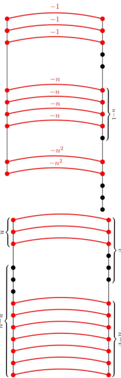
Decrease gadget D(x). For anyx∈ {0, . . . , nd−1}, the edit distance of the left and right tree
of D(x) is−x, and furthermore the right tree does not depend on the value of x. This is obtained by representingxin basenasx=Pd−1
i=0 αini. The left tree is a path composed
of d segments, the i-th segment consisting of αi nodes. The right tree is a path composed of d
segments, each consisting of n−1 nodes. Nodes from the i-th segment of the left tree can be matched with nodes from thei-th segment of the right tree with cost−ni, so the total cost is−x,
see Figure 5 (left). We reuse the same set of distinct labels in every decrease gadget of the same type, hence we need onlyO(d)distinct labels in total. Furthermore, note that the cost of matching the left tree ofD(x) with any tree is at least−x and the cost of matching any node ofD(x)is−ni
for some i∈ {0,1, . . . , d−1}.
Equality gadgetE(u, v, c=). For anyu, v∈ {1, . . . , n}andc=∈ {0, . . . , nd−1}, the edit distance of the left and right tree ofE(u, v, c=) is−c=·nifu=v and at least−c=·n+c= otherwise. Also, the left tree does not depend on v and the right tree does not depend onu.
The left tree is a path composed of a segment of length u and a segment of length n−u. The right tree is a path composed of a segment of length v and a segment of length n−v. Nodes from the first segment of the left tree can be matched with nodes from the first segment of the right tree with cost −c=, and similarly for the second segments. Then, if u = v we can match all nodes in both trees, so the total cost is −c=·n. Otherwise, we can match at most n−1 nodes, making the total cost at least −c=·n+c=, see Figure 5 (right). Furthermore, note that the total cost of matching the left tree ofE(u, v, c=)with any tree is at least −c=·nand the cost of matching any node of E(u, v, c=) is −c=.
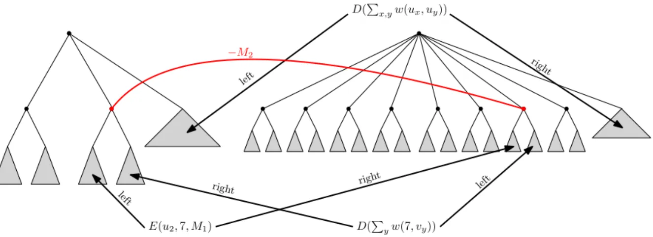
Connection gadget C(i, j, M). For anyi, j∈ {1, . . . , N}and sufficiently largeM ∈ {0, . . . , nd− 1}, the edit distance of the left and right tree of C(i, j, M)is−M−W(i, j). The left tree does not depend onj and the right tree does not depend oni.
Let {u1, . . . , uk/3} and {v1, . . . , vk/3} be the k/3-cliques corresponding to iand j, respectively, whereu1 < u2 < . . . , uk/3 and v1 < v2 < . . . < vk/3. Recall that W(i, j) denotes the total weight of all edges connecting two nodes in thei-th clique or a node in thei-th clique with a node in the j-th clique, where we assume that w(u, u) = 0. We construct the gadgetC(i, j, M) as follows. The root
−1 −1 −1 −n −n −n −n −n2 −n2 n − 1 z }| { v z }| { n − v z }| { u z }| { n− u z }| {
Figure 5: Left: Decrease gadget built for d= 3,n= 6and x=n2·2 +n·4 + 3. Right: Equality gadget foru= 3,v= 6.
of the left tree has degree1 +k/3 and the root of the right tree has degree1 +n. Their rightmost children correspond to the root of the left and the right trees of D(P
x<yw(ux, uy)), respectively.
Every other child of the left root can be matched with every other child of the right root with cost
−M2 (we fix M1 and M2 later). Intuitively, we would like the x-th child of the the left root to be matched with the ux-th child of the right root, and then contribute −Pyw(ux, vy) to the total
cost, so that summing up overx= 1,2, . . . , k/3 we obtain the desired sum. To this end, we attach the left tree ofE(ux,·, M1)and the right tree ofD(·) to thex-th child of the left root. Similarly, we attach the right tree ofE(·, t, M1)and the left tree of D(Pyw(t, vy))to the t-th child of the right
root. Here we use ·to emphasise that a particular tree does not depend on the particular value of the parameter. All decrease gadgets are of the same type. See Figure 6.
D(P x,yw(ux, uy)) E(u2,7, M1) D(Pyw(7, vy)) right right left left left righ t −M2
Figure 6: Schematic illustration of a connection gadget for k/3 = 2 andn= 8.
we have enumerated the clique corresponding to i so that u1 < u2 < . . . < uk/3). We claim that, for appropriately chosen M1 and M2, no better solution is possible. Let W = Pu,vw(u, v). We fix M1 =W ·(k/3 + 1). This is enough to guarantee that the total cost contributed by nodes in all decrease gadgets is at least−M1. The total cost contributed by nodes in all equality gadgets is at least−M1·n·k/3. Consequently, setting M2 =M1·n·k/3 +M1 guarantees that any optimal solution must match all children of the left root, so in fact, for every x = 1,2, . . . , k/3 we must match thex-th child of the left root to some child of the right root. Because matching the left tree of any decrease gadget contributes at least −W to the total cost, by the choice of M1 an optimal solution in fact must match thex-th child of the left root with the ux-th child of the right root, as
otherwise we lose at leastM1due to the corresponding equality gadget that cannot be compensated by matching its accompanying decrease gadget. Finally, the corresponding decrease gadget adds
−P
yw(ux, vy) to the total cost. Therefore, as long asM ≥M2·k/3 +M1·n·k/3 the total cost is indeed−M−W(i, j)after choosing the cost of matching the roots to be−M+M2·k/3+M1·n·k/3. For any node in a decrease gadget, the cost of matching is at least−W, for any node in an equality gadget, the cost of matching is −M1, and finally the cost of matching the children of the roots is
−M2, so the cost of matching any node of C(i, j, W) is at least −M. For the correctness of the construction it is enough thatM is at least
M2·k/3 +M1·n·k/3 =M1((nk/3 + 1)k/3 +nk/3)
=W(k/3 + 1)k/3(nk/3 + 1 +n) =W(k/3 + 1)k/3(n(k/3 + 1) + 1)
≤W ·n(k/3 + 1)3 =nO(ck).
Micro structures A0i, Dz0, Bz, C0
j. We only explain how to construct A0i and Dz0, for any i =
1,2, . . . , N and z0 = 1,2, . . . , N, as the construction of Bz and Cj0 is symmetric. Recall that we
requirecmatch(A0i, Dz0) =−M6−M4(N−i)−W(i, z0) and for every node inA0i andDz0 the cost of matching should be at least −M6.
A0i consists of a root to which we attach the left tree of D(M6+M4(N −i)−M) and the left tree ofC(i,·, M), whileDz0 consists of a root to which we attach the right tree ofD(·)and the right
tree ofC(·, z0, M). All decrease gadgets attached as the left children ofA0
i andDz0 are of the same type, and all decrease gadgets used inside the connection gadgets attached as the right children are also of the same but other type. This guarantees that the total cost of matching A0i to Dz0 is simply−M6−M4(N−i) +M−M−W(i, j) =−M6−M4(N−i)−W(i, j). For sufficiently large
M ≥W ·n(k/3 + 1)3, the cost of matching any node inD(M6+M4(N−i)−M) is at least−M6 and the cost of matching any node in C(i, j, M)is at least M.
Micro structures Ai, Cj. Here the situation is a bit more complex, as we simultaneously require
thatcmatch(Ai, Cj) =−M2−W(j, i) +W(j−1, i−1)for every i= 2,3, . . . , N and j= 2,3, . . . , N
andcmatch(Ai, C1) =−M5−M3(i−1)−W(1, i), andcmatch(A1, Cj) =−M
5−M3(j−1)−W(j,1) for everyi= 1,2, . . . , N and j = 1,2, . . . , N. We must also make sure that the cost of matching a node ofAi to a node ofCj should be at least−M2, except that the root ofAi (Cj) can be matched
to the root of C1 (A1) with cost larger than −M5 −M but at most −M5 and, for any non-root node of Ai (Cj) and for any non-root node of C1 (A1), the cost of matching is larger than −M4.
For every i > 1 (j > 1), Ai (Cj) consists of two subtrees, called left and right, attached to
the common root, while A1 (C1) consists of a single subtree connected to a root. For everyi > 1 (j >1), the left subtree ofAi (the right subtree of Cj) consists of a root with two subtrees, called
left-right and left-right (right-left and right-right). For every i > 1, nodes of the right subtree of
Ai can only be matched to nodes ofC1 and nodes of the left subtree of Ai can only be matched to
nodes of the right subtree of Cj for any j >1. For everyj >1, nodes of the left subtree of Cj can
only be matched to nodes ofA1 and nodes of the right subtree ofCj can only be matched to nodes
of the left subtree of Ai for any i >1. Nodes ofA1 can be matched to nodes of the left subtree of
Cj, for any j >1. Nodes ofC1 can be matched to nodes of the right subtree of Ai, for any i >1.
Additionally, the root ofA1can be matched to the root ofC1with cost−M5−W(1,1)>−M5−M, and for any i > 1 (j > 1), the root of Ai (Cj) can be matched to the root of C1 (A1) with cost
−M5. The subtrees are constructed as follows:
1. the right subtree of Ai is the left tree ofD(M3(i−1) +W(1, i)),
2. the only subtree ofA1 is the right tree of D(·),
3. the left subtree ofCj is the left tree ofD(M3(j−1) +W(j,1)),
4. the only subtree ofC1 is the right tree of D(·).
It remains to fully define the left subtree of everyAi and the right subtree of everyCj, for i, j >1.
Recall that the goal is to ensure cmatch(Ai, Cj) = −M
2−W(j, i) +W(j−1, i−1). We define a newn-node graph with weight function w0(u, v) =M−w(u, v) for anyu6=v (for sufficiently large
M, the new weights are positive). Then, let C0(i, j, M) denote the connection gadget C(i, j, M) constructed for the new graph. Nodes of the left-left (left-right) subtree ofAi can be only matched
to nodes of the right-left (right-right) subtree of Cj. The subtrees are constructed as follows:
1. the left-left subtree ofAi is the left tree ofC(i,·, M·(k/3)2),
2. the right-left subtree ofCj is the right tree of C(·, j, M·(k/3)2),
3. the left-right subtree ofAi is the left tree ofC0(i−1,·, M2),
See Figure 7. For the construction of C(i, j, M ·(k/3)2) and C(i−1, j−1, M2) to be correct we need that M ·(k/3)2 ≥W ·n(k/3 + 1)3 and M2 ≥M ·n2·n(k/3 + 1)3, respectively, which holds for sufficiently largeM.
Now we calculatecmatch(Ai, Cj). C(i−1, j−1, M2)contributes−M2minus the total cost of edges
connecting two subsets ofk/3nodes in the new graph. As the weights in the new graph are defined asw0(u, v) =M−w(u, v), this is exactly−M2−(M·(k/3)2−W(i−1, j−1)). C(i, j, M·(k/3)2) contributes−M·(k/3)2−W(i, j), so c
match(Ai, Cj) =−M·(k/3)
2−W(i, j)−M2−(M·(k/3)2−
W(i−1, j−1)) =−M2−W(i, j) +W(i−1, j−1)as required.
It remains to bound the cost of matching nodes. Nodes in the left subtree of Ai (Cj) can be
matched only to nodes of C1 (A1) with cost at least −M3 ·n >−M4, except that the roots can be matched with cost −M5. The cost of matching a node of A
i to a node of Cj, for i, j > 1, is
either at least −M ·(k/3)2 (for the nodes ofC(i, j, M·(k/3)2) or at least −M2 (for the nodes of
C(i, j, M2)), so for sufficiently largeM at least−M2.
C(i, j, M3·(k/3)2) C1 A1 Ai Cj D(M3(i−1) +W(1, i)) righ t left D(M3(j−1) +W(j,1)) righ t left C0(i−1, j−1, M4) left
right left righ
t −M 5 −M 5 −M5−W(1,1)
Figure 7: Micro structuresA1, C1 and Ai, Cj for i, j >1.
Wrapping up. We have shown how to construct, given a complete undirected n-node graph G, two trees such that the weight of the max-weight k-clique in G can be extracted from the cost of an optimal matching (and, as mentioned in the beginning of Section 2, by a simple transformation this is equal to the edit distance). To complete the proof of Lemma3, we need to bound the size of both trees and also the size of the alphabet used to label their nodes.
Initially, each tree consists of 2N original spine nodes, where N ≤nk/3,2N leaf nodes, and N additional spine nodes. Then, we attach appropriate microstructures to the original spine nodes and leaf nodes. The microstructures areA0i, I, Cj0, Ai, Bz, Cj, Dz0. Every copy ofI consists ofk/3·n nodes. To analyse the size of the remaining microstructures, first note that if x∈ {0, . . . , nd}then
the decrease gadget D(x) consists ofO(d·n) nodes. The equality gadget always consists of O(n)
nodes. Finally, the connection gadgetE(·,·, M)withM ∈ {0, . . . , nd}consists ofO(n(n+d·n) +d·
n) =O(d·n2)nodes. LetM =ndwithdto be specified later. Now, the size of the microstructures
can be bounded as follows: A0i andDz0 (and alsoBz andCj0) consist ofO(6d·n+d·n2) =O(d·n2) nodes. The right subtree of Ai (and the left subtree of Cj) consists of O(3d·n) nodes, while the
left subtree of Ai (and the right subtree of Cj) consist ofO(k2d·n2+ 2d·n2) =O(k2d·n2) nodes.
Thus, the total size of all microstructures is O(N ·k2d·n2). It remains to bound M. Recall that we require M ≥ W ·n(k/3 + 1)3, M ·(k/3)2 ≥ W ·n(k/3 + 1)3 and M ≥ n3(k/3 + 1)3, where
W ≤n2·nO(ck)=nO(ck). Hence, it is sufficient thatM ≥8W·n3k3. Settingd= Θ(ck)is therefore enough. The size of the whole instance thus is O(nk/3+2·ck) =O(nk/3+2).
We also have to bound the size of the alphabet. We needk/3distinct labels for the nodes ofI. We need O(d) distinct labels for the nodes of all decrease gadgets of the same type. There is a constant number of types, and all other nodes require only a constant number of distinct labels (irrespectively onc and k), so the total size of the alphabet isO(ck) =O(1).
4
Algorithm for Caterpillars on Small Alphabet
In this section, we show that the hard instances of TED from Section 2 can be solved in time
O(n2|Σ|2logn), where n is the size of the trees and Σ is the alphabet. Recall that in such an instance we are given two trees F and G both consisting of a single path (called spine) of length
O(n) with a single leaf pending from every node, and all these leafs are to the right of the path in
F and to the left of the path inG (see Figure 2). In the following we use the same notation as in Lemma1. At a high level, we want to guess the rootmost non-spine node in the left tree fi0p+1 and the rootmost non-spine node in the right tree gj0p+1. The optimal matching of spine nodes above these non-spine nodes can be precomputed inO(n2)total time with a simple dynamic programming algorithm. It might be tempting to say the same about the situation below, but this is much more complicated due to the fact that leaf nodes in this part are matched in reversed order. To overcome this difficulty, we need the following tool.
Lemma 6. For strings s[1..n] and t[1..m] over alphabet Σ and matching cost cmatch(c, d) for any two lettersc, d∈Σ, we define the optimal matching ofsand the reverse oft as
minn k X `=1 cmatch(s[i`], t[j`]) k≥0, 1≤i1 < . . . < ik ≤n, 1≤jk< . . . < j1 ≤m o .
Given two strings s[1..n], t[1..n], in O(n2logn) total time we can calculate, for every i and j, the
optimal matching of s[1..i]and the reverse of t[1..j].
Proof. We construct an(n+ 1)×(n+ 1)grid graph on nodesvi,j, wherei, j= 0,1, . . . , nas follows.
For every i, j= 0,1, . . . , n, we create a directed edge fromvi,j to vi+1,j andvi,j+1 with length zero. Also, we create a directed edge fromvi,j tovi+1,j+1 with lengthcmatch(s[i], t[n+ 1−j]). Then, paths