Position Control of an Unmanned Aerial Vehicle From a Mobile Ground Vehicle

(1)

Michigan Technological University Michigan Technological University

Digital Commons @ Michigan Tech

Dissertations, Master's Theses and Master's Reports

2017

Position Control of an Unmanned Aerial Vehicle From a Mobile

Ground Vehicle

Astha Tiwari

Michigan Technological University, asthat@mtu.edu

Recommended Citation Recommended Citation

Tiwari, Astha, "Position Control of an Unmanned Aerial Vehicle From a Mobile Ground Vehicle", Open Access Master's Thesis, Michigan Technological University, 2017.

https://digitalcommons.mtu.edu/etdr/470

Follow this and additional works at: https://digitalcommons.mtu.edu/etdr

Part of the Controls and Control Theory Commons, and the Other Electrical and Computer Engineering Commons

(2)

POSITION CONTROL OF AN UNMANNED AERIAL VEHICLE FROM A MOBILE GROUND VEHICLE

By Astha Tiwari

A THESIS

Submitted in partial fulfillment of the requirements for the degree of MASTER OF SCIENCE

In Electrical Engineering

MICHIGAN TECHNOLOGICAL UNIVERSITY 2017

(3)

(4)

This thesis has been approved in partial fulfillment of the requirements for the Degree of MASTER OF SCIENCE in Electrical Engineering.

Department of Electrical and Computer Engineering

Thesis Advisor: Dr. Timothy C. Havens

Committee Member: Dr. Jeremy Bos

Committee Member: Dr. Zhaohui Wang

(5)

(6)

Dedication

To my family, teachers and friends

for their unconditional love and unwavering faith in me without which I would neither be who I am nor would this work be what it is today.

(7)

(8)

List of Figures

2.1 Configuration of a Quadcopter [16] . . . 18

2.2 Motion Principle for the Quadcopter [16] . . . 19

3.1 Control Structure for the Quadcopter . . . 28

4.1 Block diagram of quadcopter . . . 34

4.2 Postion Control Subsystem of the Quadcopter . . . 35

4.3 Attitude Control Subsystem of the Quadcopter . . . 36

4.4 Quadcopter Control Mixing Subsystem . . . 37

4.5 Quadcopter Dynamics Subsystem . . . 39

4.6 Quadcopter Motor Dynamics Subsystem . . . 39

4.7 Plot of Position Controller Action inx direction . . . 40

4.8 Plot of Position Controller Action iny direction . . . 41

4.9 Plot of Position Controller Action inz direction . . . 41

5.1 Marker constellation of 5 elements arranged on a 3D axis with length of 25 cm for each leg. . . 44

(13)

5.3 Detected and tracked position of a quadcopter in x-direction . . . . 51

5.4 Detected and tracked position of a quadcopter in y-direction . . . . 51

5.5 Detected and tracked position of a quadcopter in z-direction . . . . 52

6.1 Two Wheel Differential Drive . . . 55

6.2 Vehicle in an Initial Frame of Reference . . . 56

6.3 Closed Loop Feedback Control Architecture . . . 60

7.1 Case 1:Results for Closed Loop for Varyingy . . . 63

7.2 Case 1: Mean Squared Error for Varying y . . . 63

7.3 Case 1: Results for Closed Loop whenx= 4 . . . 64

7.4 Case 1: Mean Squared Error forx-axis . . . 64

7.5 Case 1: Results for Closed Loop whenz = 20 . . . 65

7.6 Case 1: Mean Squared Error forz-axis . . . 65

7.7 Case 2: Results for Closed Loop wheny= 4 . . . 67

7.8 Case 2: Mean Squared Error fory-axis . . . 68

7.9 Case 2: Results for Closed Loop whenx Varies . . . 68

7.10 Case 2: Mean Squared Error for x-axis . . . 69

7.11 Case 2: Results for Closed Loop when z = 20 . . . 69

7.12 Case 2: Mean Squared Error for z-axis . . . 70

7.13 Case 3: Results for Closed Loop when y varies . . . 71

7.14 Case 3: Mean Squared Error for y-axis . . . 72

7.15 Case 3: Results for Closed Loop when x varies . . . 72 xii

(14)

7.19 Conventional PID with Feed Forward Control . . . 75

7.22 Case 4: Results for Closed Loop when x varies . . . 77

7.30 Case 5: Results for Closed Loop when z varies . . . 82

(15)

7.38 Case 6.1: Results for Closed Loop when y varies . . . 88

7.39 Case 6.1: Mean Squared Error for y-axis . . . 88

7.40 Case 6.1: Results for Closed Loop when x varies . . . 89

7.41 Case 6.1: Mean Squared Error for x-axis . . . 89

7.42 Case 6.1: Results for Closed Loop when z varies . . . 90

7.43 Case 6.1: Mean Squared Error for z-axis . . . 91

7.57 Case 7.2: Mean Squared Error for y-axis . . . 100 xiv

(16)

(17)

(18)

List of Tables

7.1 Error Matrix for Changing Focal Length . . . 95 7.2 Error Matrix with Changing Resolution . . . 103 7.3 Overall Simulation Error Matrix . . . 106

(19)

(20)

Acknowledgments

I would like to gratefully thank various people who have helped me out throughout this excursion. First and foremost, I would like to thank my parents and family for their immense support and encouragement. I owe my most profound appreciation to my advisor Dr. Timothy Havens, who has been exceptionally patient and guided me at each progression of the process. Without his support, positivity and enthusiasm my work would not have been completed. I am deeply grateful to my committee members, Dr. Jeremy Bos and Dr. Zhaohui Wang for being so warm and co-operative.

I owe a great debt of gratitude to my lab-mates Joshua Manela and Joseph Rice for helping me out on whatever point I was stuck with any problem. I am indebted to Donald Williams for his unwavering support and motivation which helped me to be on focussed toward my work. Last but not the least, I am eternally thankful to all my friends for bearing with me through the last couple of years and helping me make this possible.

(21)

(22)

Abstract

The core objective of this research is to develop a closed loop feedback system between an unmanned aerial vehicle (UAV) and a mobile ground vehicle. With this closed loop system, the moving ground vehicle aims to navigate the aerial vehicle remotely. The ground vehicle uses a pure pursuit algorithm to traverse through a pre-defined path. A Proportional-Integral-Derivative (PID) controller is implemented for position control and attitude stabilization of the unmanned aerial vehicle.

The problem of tracking and pose estimation of the UAV based on vision sensing is investigated. An estimator to track the states of the UAV using the images obtained from a single camera mounted on the ground vehicle is developed. This estimator coupled with a Kalman filter determines the UAV’s three dimensional position. The relative position of the UAV from the moving ground vehicle and control output from a joint centralized PID controller is used to further navigate the UAV and follow the motion of the ground vehicle in closed loop to avoid time delays. This closed loop system is simulated in MATLAB and Simulink to validate the proposed control and estimation approach. The results obtained validate the control architecture proposed to attain a closed loop feedback between the UAV and the mobile ground vehicle. UAV closely follows the ground vehicle and various simulation support the parameter settings.

(23)

(24)

Chapter 1 Introduction

Over the past decade interest in UAV has grown significantly primarily because of its increased availability. Vision based control for quadcopter is an extremely interesting problem with a wide range of practical applications. Quadcopters, in particular are much more promising where human access is limited. Quadcopters are now being deployed for tasks such as remote inspection and monitoring, surveillance, mapping and target tracking.

Quadrotors have been developed with controls aiding good maneuverability, simple mechanics, and the ability to hover, take-off and land vertically with precision. Due to their small size, they can get close to targets of interest and also remains undetected at low heights. The main drawbacks for a quadcopter are its high-power consumption

(25)

and payload restriction. Due to limited payload capability, the number of sensors on-board are restricted. To overcome this limitation vision-based techniques and remote control for the quadcopter are primary areas of research these days.

Vision-based sensors are low in cost and weight and can be easily deployed with quadcopters for diverse applications, especially in GPS-denied areas, like indoor en-vironments. A common application for quadcopters currently is for target detection and tracking. Vision-based remote navigation for a quadcopter is well suited for such tasks. UAV’s can be used for sensing from above; hence, we propose an application whera a UAV flies in front of a moving ground vehicle in order to sense hazards or objects. The portion of this problem solved in this thesis is the tracking and control of the UAV.

Work presented in this thesis deals primarily with the development of a tracking (or localization) and control method for a UAV in collaboration with a moving ground vehicle. To approach this problem a closed loop feedback control system for a quad-copter to follow a moving ground vehicle is developed. A novel algorithm is de-veloped for vision-based estimation for detecting and tracking of the quadcopter by using image processing. Six degree-of-freedom(6DOF) tracking of the quadcopter is accomplished with a monocular camera mounted on the ground vehicle, which tracks coloured markers on the UAV. This tracking result is then passed to a Kalman filter, which is used to estimate the pose of the UAV.This approach gives very precise pose

(26)

estimation of position, altitude, and orientation of the quadcopter with respect to its counterpart on ground.Finally, a control input for PID controller is communicated to the UAV in order to maintain a predetermined path; e.g. maintaining a position of 25 meters in front of the vehicle, or weave back and forth in front of the vehicle.

1.1 Literature Review

1.1.1 Quadcopter Control

Quadcopter control and its implementation in various applications have made sig-nificant progress over time. Nowadays autonomous navigation for a quadcopter is extremely easy to attain with multiple algorithms and methods from which to choose. A quadrotor has four equally spaced rotors placed at the corners of a square struc-ture. It generally uses two pairs of identical propellers. Two of these propellers spin clockwise and the another two in a counter-clockwise direction. By varying the speed of each rotor, any desired thrust can be generated to lift and maneuver the craft. To navigate the quadcopter, we need to control these four independent rotors.

In general, fundamental quadcopter control in itself is a difficult problem. With six de-grees of freedom, three rotational and three translational, and only four independent inputs make this system severely underactuated. The rotational and translational

(27)

degrees of freedom are coupled making the system dynamics non-linear in nature. Except for air friction, which is negligible, quadcopters do not have friction to sup-press or aid their motion; so, they must provide their own damping for stability and movement.

In [3], authors presented the modelling and simulation of an autonomous quadrotor micro-copter in a virtual outdoor scenario. They also developed flight simulator to include controller design and model validation. In [13] and [26], a study of the kinematics and dynamics of a quadrotor are discussed for better understanding of the underlying physics and mathematics involved in the modelling of a quadrotor. These work deal with the implementation of flight dynamics but bot the control for the navigation.

Several researchers have presented their approach to achieve control for the quad-copter. Research presented in [31] and [6] applies a PID controller for attitude sta-bilization of a quadcopter. In both these work position control to fly the quadcopter is not talked about. Their control model is limited for hovering applications only. A simple PID control is also sufficient for hovering and attitude control. Using more sophisticated controllers improves the performance, but increases the computation power needed. These controllers are tougher to design and deliver very little im-provement in minimal close to hover flight conditions. There will always be a tradeoff between computational capacity and performance requirements. Emphasis was also

(28)

on adaptive control schemes for quadcopter control. It is believed that such control can improve the quadcopter performance in terms of model uncertainties, varying pay-loads, and disturbance rejections. Research shown in [25] shows that both PID and adaptive control give similar results. Very little improvement was observed when using the adaptive control. Also, the controller developed is not robust and depends on varying the parameters for different navigation tasks. Experiments in [36] and [41] confirm that quadcopter stability can be achieved with PID controller for tar-get tracking tasks but the results of these work lack the optimal tuning of the PID controller parameters.

Work in [42] defines the feedback linearization base control method for landing a UAV on a base vehicle moving with a constant speed. This method reduces the problem to a fixed pre-defined trajectory for the quadrotor. This method is difficult to implement correctly because we can not identify the actual parameters in the decoupling matrix for the UAV.The authors in [43] successfully demonstrates autonomous landing of UAVs on moving ground vehicles. Takeoff to a fixed attitude and then tracking and landing are achieved solely using PID controller for the attitude and position control. A PID controller is shown to be sufficient to achieve linear flight regime in hover condition as demonstrated in [22].

To overcome these issues of robustness and computational load for the control, in this thesis we implement PID control for both position control and attitude stabilization.

(29)

The daunting task with the PID controller is to tune the parameters in such a way; so, as to achieve a robust position control for a quadcopter. To optimally tune the parameters, Ziegler-Nicols rule was used for both attitude and position control of the quadcopter. This tuning gave the PID loop best disturbance rejection and made the system extremely robust. In all the previous cited studies, quadcopter control is the focus onto but vision based integration using image processing techniques are not discussed.

1.1.2 Tracking and Vision-Based Estimation

Our objective is to develop a vision-based algorithm for localization of the quadcopter with respect to the ground vehicle. Using multiple frames makes the entire problem difficult to implement and computationally very expensive. So, we implement image processing for one frame at a time. Heavy computational-load algorithms can not be used on low power computers onboard a typically small quadcopter. The main challenge addressed here is tracking and estimating the relative altitude between the quadcopter and ground vehicle based on monocular camera measurements. For this purpose, sensor fusion of a monocular camera with GPS or other laser-based sensors can be used for estimation to increase accuracy in measurements obtained.

(30)

Firstly we had to be certain that vision-based sensors would be best for our applica-tion. For this purpose we scrutinized other sensors such as radar. A modified aircraft tracking algorithm to include radar measurements taken from a stationary target po-sition are used in both [17] and [35]. For this algorithm, it is important that the target is in close vicinity of the measuring device, which is not always possible. To overcome this, the authors of [39] develop an alternative to fixed sensor location by assuming moving target indicators or position measurements to be directly available from aircraft sensor. Drawback of using radar as inferred from the above cited work was its limited area of operation. Also, using the radar increased the payload for the craft.

It is to be noted that in general for target tracking problems, cameras have an ad-vantage over active range sensors, as they are passive and thus targets are unaware of observation. Currently, Simultaneous Localization and Mapping(SLAM) techniques are widely used and implemented for monocular vision systems, as discussed in [29] and [5]. In [5], authors assume that an air vehicle maintains hover position and all features are in one plane. This reduces the problem to two dimensions but makes the controller application very limited. Similarly, in [29], the authors use artificially placed features of known dimension to reconstruct three-dimensional pose for the air-craft from a two-dimensional image obtained from a monocular camera. Both these approaches propose an algorithm to simplify the pose estimation problem for a quad-copter. In [33], an algorithm is presented which relies on visual markers and wireless

(31)

transmission of camera images to a ground computer, which then remotely controls the UAV. In [21], [44] and [11], monocular visual stabilization techniques that measure relative motion are discussed and developed. These systems utilize an on-board cam-era setup for simultaneous localization and mapping (SLAM) with the UAV. Similar research has been conducted with stereo camera systems, which are computationally more expensive. Work presented in [24] and [32] use ground mounted fixed stereo cameras to remotely control the quadcopter from a ground computer, whereas in [10] a forward-facing stereo camera is mounted on the quadcopter to achieve closed-loop control for quadcopter motion with final processing on the ground station. In all these above mentioned work the camera is mounted on-board the UAV facing downwards. This arrangement also increases the payload and thereby effecting the size and power consumption for the UAV. The algorithms developed are computational expensive due to SLAM implementation.

In [23] and [20], the researchers propose a vision based autopilot relying only on optic flow. The main limitation of this method is that for accurate altitude stabilization, the quadrotor should have significant motion in the field of view, which fails for a hover condition. The work presented in [8] and [7] is very interesting as it aims at tracking a moving ground vehicle with markers from a UAV using solely vision sensing. The control takes action by gathering images from a camera mounted on the UAV and then, by appropriate image processing techniques estimates the position and velocity of the ground vehicle. The algorithm developed here is very efficient

(32)

but overlooks to include backup in cases of insufficient data when images could not be obtained.Quadcopters are finding applications in various fields while implementing SLAM. To overcome the payload restrictions, mounting the camera on the quadcopter will be troublesome to implement in an experimental setup. Hence, in this case, a camera on a ground vehicle is beneficial.

1.1.3 Closed Loop Feedback Control for UAV and ground

vehicle

With the vision-based estimation and tracking the next section of this thesis was to develop a closed loop feedback control for UAV and a moving ground vehicle for navigating a UAV remotely.Numerous controller designs for autonomous landing of a UAV on a moving target have been developed.In [9] and [27], a UAV and Unmanned Ground Vehicle(UGV) work in collaboration and should know about mutual positions and estimate relative pose of the UGV to the UAV, and in [34] mutual localization is achieved to determine the relative position of the UAV with respect to the UGV. When estimating the position of the UGV from the camera on-board the UAV for closed loop control system, many researchers have worked with color detection for image processing. It consists in placing colored markers on a the UGV surface. These techniques are discussed in [30] and [12], where they go through the acquired videos from the UAV until a match is found with tracked color. Once the location of the

(33)

tracked object is found, the relative pose of the UGV is extracted. Color tracking methods are mostly reliable due to easy implementation but have some drawbacks. This method is sensitive to lighting conditions and depends on the environment. In [40], the author discusses a feature-based (black and white pattern) detection for multiple robot localization. The presented method allows the tracking of several features at a time with good precision and accuracy. The above mentioned works deal with tracking of the ground vehicle and hence deals only for two dimensions.

In [37], the authors propose a nonlinear control technique for landing a UAV on a moving boat. Here the attitude dynamics are controlled using fast time scale with guaranteed Lyapunov stability. The authors present the simulation results for the same with guaranteed robustness for bounded tracking errors in the attitude con-trol. The method relies on time scale separation of attitude and position control which makes the controller algorithm computationally expensive and dependent on the communication protocol used. A tether is used for communication between the boat and UAV. Similarly, authors in [28] work to derive a control technique for coor-dinated autonomous landing on a skid-steered UGV. First a linearized model of the UAV and the UGV are developed and then control strategies are incorporated in the closed loop to study the coordinated controller action. In this work, the non-linearities of the quadcopter are overlooked.

The effects of airflow disturbances are investigated and shown in [19] with non-linear

(34)

controller design and simulation for landing the quadcopter on a moving target. [15] focuses on developing an estimation technique to track the position and velocity of a moving ground target as viewed from a single monocular camera on-board the UAV. Here an inertial measurement unit (IMU) with three axes accelerometer and rate gyro sensors along with a GPS unit give the states for the UAV which, when combined with the camera estimates, give the target states. Similarly, in both [4] and [1], the author develops an object tracking controller using an on-board vision system for the quadcopter. It also demonstrates stable closed loop tracking for all three control axes, individually and collaboratively. These work don’t aim at reducing the size of the quadcopter and minimizing the power needed for its operation as in all these work the camera is mounted on the UAV and also the pose estimation is done by the camera on-board the quadcopter.

Work in [18] takes the coordinated control for a UAV and UGV a step further by presenting an algorithm for tracking a ground vehicle from a camera mounted on the UAV with a constant stream of video of the motion. The conventional vision based tracking algorithm also uses a fuzzy logic controller for a more precise result. This makes the control action computationally expensive and slows down the process. Work presented in thesis intends to attain target tracking based only on vision sensing from a single camera mounted on the ground vehicle. Accurate altitude and yaw estimation of the UAV is achieved using image processing algorithms discussed in chapter 5.

(35)

1.2 Motivation and Research Objective

Navigation and position control of an unmanned aerial vehicle has been a subject of intense study in the past decades. Typically sensors on board of the aerial vehicle include an inertial measurement unit(IMU) with three axes accelerometers and rate gyro sensors, a global positioning system (GPS), and a camera, which are used to give the position for the vehicle. Various sensor fusion algorithms are deployed for the control of the UAV position. Due to payload restriction and with intent to reduce the size, researchers are focussing on techniques to remotely control and localize the UAV.

In the literature review, recent developments in the field of quadcopter control and vision based tracking were discussed. In this research, we intend to accomplish reliable target tracking of a quadcopter using a single monocular camera onboard a moving ground vehicle unlike for most cases as discussed in section 1. Position, altitude, and rotation for the target quadcopter relative to the ground vehicle are estimated based on images obtained and further processing for vision based tracking. Algorithms and control designs are implemented and simulated in MATLAB and Simulink.

A novel algorithm presented in this thesis proposes an efficient and accurate pose estimation of the quadcopter from a ground vehicle. In [45], an assumption is made

(36)

that the yaw of the quadcopter is inherently known and thus there is no need to estimate. From this research, an understanding is developed to implement a consistent quadcopter controller for attitude stabilization and position navigation. Coordinated landing of a quadcopter on a moving ground vehicle is discussed in [2], [38] and [28]. In these works the camera is mounted on the ground vehicle or at the ground station but the camera is stationary. Conventionally, quadcopters carry a camera on them for vision based navigation, but for the work in this a thesis camera is mounted on the moving ground vehicle. The camera faces up and forwards and provides images of the moving quadcopter. This simplifies the problem statement as it aids in pose estimations from ground vehicle and simplifies the quadcopter control problem. This also helps in ground air interactions for multi-agent systems. Also, to deal with situations of temporary target loss the vision-based tracking algorithm was coupled with Kalman filter to estimate position.

1.3 Thesis Outline

In this thesis, we implemented a vision-based tracking and remote navigation method for quadcopter control from a ground vehicle. The vision-based estimation algorithm is successfully achieved with anticipated control strategies and tolerable error in pose estimation. Then using predefined path from a ground vehicle is used to navigate the quadcopter. More complex control algorithms can be implemented for future

(37)

work. There are various approaches to deal with quadcopter attitude and position control and stabilization; work presented here focus on integration of image process-ing algorithms with a novel PID controller for quadcopter navigation from a remote moving ground vehicle. For this purpose, PID control laws are implemented on the quadcopter for both position control and attitude stabilization.

This thesis is divided into 7 chapters. In the first chapter an introduction to the thesis is given discussing the literature review of the previous work done in the field, moti-vation behind the project, and an outline for the project itself. Chapter 2 discusses the mathematical model for a quadcopter. Derivation for a quadcopters non-linear equation of motion are given.

Chapter 3 focus on the control laws for the non-linear dynamic model of the quad-copter. Here we have modeled a classic controller for attitude stabilization and posi-tion tracking. In Chapter 4, the mathematical model derived for the quadcopter and its position control are modeled in Simulink. Chapter 5 develops an algorithm for vision-based estimation and tracking of the quadcopter. We develop our image pro-cessing for detection and tracking of the quadcopter in MATLAB. Also, we validate the algorithm by simulating a video of a randomly moving quadcopter and results of this simulation are included.

Chapter 6 aims at developing the overall control architecture for position control of a quadcopter in closed loop feedback with a moving ground vehicle. Initially we derive

(38)

the kinematic equations for the ground vehicle and then outline the overall system. Chapter 7 shows simulation and results of the overall model developed in various cases to validate the work. Finally, Chapter 8 provides a summary of the project and explores the possible future research in this field.

(39)

(40)

Chapter 2 Quadcopter Dynamics

Quadcopters are under-actuated systems in which four independent inputs are used to control motion in six degrees of freedom, three translational and three rotational. The resulting dynamics are highly nonlinear primarily because of aerodynamic ef-fects. Quadcopters are lifted and propelled using four vertically oriented propellers. Quadrotors use two pairs of identical fixed pitched rotors, two in clockwise direction placed diagonally with respect to each other and the other two in counter-clockwise direction placed diagonally. Figure 2.1 [16] shows the configuration of the quadcopter.

To control and maneuver the quadcopter, independent variation in the speed of ro-tor can be changed accordingly. Change in speed of each rotor affects the total

(41)

Figure 2.1: Configuration of a Quadcopter [16]

thrust which can be further controlled to create desired total torque to navigate the quadcopter in all three directions. Figure 2.2 [16] shows the motion principle for a quadcopter. By varying the roll, movement in x direction can be controlled. Simi-larly, by controlling the pitch of the craft ,movement in y direction is achieved. To increase the roll, the thrust on motor 1 is decreased and for the diagonally placed motor 3, thrust is increased. This results in a moment which tilts the quadcopter by creating a component of thrust in the x direction. Motor 2 and motor 4 work together in a similar manner to maintain the position in the ydirection. Quadcopter Dynamics are discussed and a mathematical formulation for the Quadcopter model is derived and discussed in detail in [16]. Maintaining the altitude of the quadcopter, i.e., its position in the z-axis is achieved by equally distributing the thrust needed on all four motors. Decreasing the thrust on one pair of motors and increasing the thrust by an equal amount on the other two motors creates a moment about z-axis of the quadcopter triggering it to yaw. To determine all the equation governing the

(42)

Figure 2.2: Motion Principle for the Quadcopter [16]

motion of the quadcopter we need to analyze it in the inertial reference frame and the fixed body frame. The inertial reference frame is defined by the ground with gravitational force in the negative z-axis and the fixed body frame is defined when the rotor axes point in the positive z-axis and the arms pointing in the x and y di-rection. The inertial reference frame is used to measure the position and velocity of the quadcopter whereas to determine the orientation and angular speeds we need to assess the body-fixed frame. Lets define the state vectors as follows:

Position Vector:x= [x, y, z]T & Velocity Vector:v= [vx, vy, vz]T, (2.1)

Orientation Vector:α= [φ, θ, ϕ]T & Angular Velocity Vector:ω= [ωx, ωy, ωz]T,

(2.2) Where X, the position vector, is defined relative to the inertial reference frame and

(43)

the other three vectors are defined relative to the fixed body frame. Also, the stan-dard Euler angles, with notations φ, θ and ϕ are called pitch, roll and yaw of the quadcopter, respectively. The angular velocity vectorω 6= ˙α and instead is the vector pointing along the axis of rotation, given by the following relation.

ω =         1 0 −sin(θ)

0 cos(φ) cos(θ) sin(φ) 0 −sin(φ) cos(θ) cos(φ)

        ˙ α. (2.3)

The matrix above can also be called the transformation matrix from the inertial frame to the fixed-body frame and the transformation matrix from the body frame to the inertial frame is given by

˙ α=Wnω =        

1 sinφtanθ cosφtanθ

0 cosφ −sinφ

0 sin_cosφ_θ cos_cosφ_θ         ω. (2.4)

Similarly, we can determine the relation between the fixed-body frame and the inertial frame by using the rotation matrixR, going from the body frame to the inertial frame. The rotation sequence of any aircraft is described as a rotation about thez-axis (yaw) followed by the rotation abouty-axis (pitch) and eventually by the rotation about the

x-axis (roll). Using the three rotations, a composite rotation matrix can be formed

(44)

which goes from the fixed body frame to the inertial frame and is given by R=        

cosϕcosθ (cosϕsinθsinφ−sinϕcosφ) (cosϕsinθcosφ+ sinϕsinφ) sinϕcosθ (sinϕsinθsinφ+ cosϕcosφ) (sinϕsinθcosφ−cosϕsinφ)

−sinθ −cosθsinφ cosθcosφ

        . (2.5) It is to be noted that this rotation matrix is orthogonal and henceR−1 =RT, which is the rotation matrix from the inertial reference frame to the fixed-body frame. Together, the relationship between linear velocities and angular rates in the inertial and fixed-body frame are given by

    ˙ X ˙ α     =     R(α) 0 0 Wn(α)         v ω     . (2.6)

The equations of motion for the quadcopter are expressed in terms of fixed-body velocities and angular rates. We implement the Lagrangian approach extended to quasi-coordinates for the equation of motion. Here we can not directly use the angular velocities to determine the value for orientation vector, so we use the quasi-coordinate formulation, where the components of angular velocities are defined in terms of the derivative values with respect to time. The equations can be written as follows

(45)

L= 1 2mv

T_v₊1

2ω

T_I_ω₊_mgz. _(2.8)

In the above equation,mis the mass of the quadcopter andIis its moment of inertia. Now we need to determine its moment of inertia. For this, the quadcopter is assumed to have a perfectly symmetrical structure along all 3 axes and its center of mass is located at the geometric center of its arms. Thus, the inertia matrix becomes a diagonal matrix with Ixx =Iyy , and the inertia matrix can be reduced to

I=         Ixx 0 0 0 Iyy 0 0 0 Izz         . (2.9)

Now, if we implement the quasi-coordinate Lagrangian formulation, we obtain the following equations, d dt( ∂L ∂v) T ₊_ω₍∂L ∂v)−(T1) T₍∂L ∂X) =τ1, (2.10) d dt( ∂L ∂ω) T ₊_v₍∂L ∂v) +ω( ∂L ∂ω)−(T2) T₍∂L ∂α) = τ2. (2.11)

When we expand 2.10 and 2.11 for each variable of the state vector using the proper-ties of partial derivatives, we obtain the following six equations governing the motion of a quadcopter:

m[ ˙vx−vyωz+vzωy−gsin(θ)] = 0, (2.12)

(46)

m[ ˙vy −vzωx+vxωz+gcos(θ) sin(φ)] = 0, (2.13) m[ ˙vz−vxωy +vyωx+gcos(θ) cos(φ)] = u1, (2.14) Ixxω˙x+ (Izz−Iyy)ωyωz =u2, (2.15) Iyyω˙y+ (Ixx−Izz)ωxωz =u3, (2.16) Izzω˙z =u4, (2.17) τ =                     0 0 u1 u2 u3 u4                     =                     0 0 T1+T2+T3+T4 (T4−T2)l (T3−T1)l (T2+T4−T1−T3)µ                     . (2.18)

In 2.12 - 2.18 aboveT1−4 are the forces applied by the four motors on the quadcopter,

µ is the torque coefficient and is a constant value for a particular setup, andl is the length of the arm from the center of gravity to the motors. Since the quadcopter is assumed to be symmetric the length is same for all four motors. All the equations written above are derived and formulated in fixed-body frame and can be easily

(47)

converted into the inertial frame as shown in the following steps:     R−1 0 0 (Wn)−1         ˙ X ˙ α     =     v ω     , (2.19)     R−1 0 0 (Wn)−1         ¨ X ¨ α     −     ˙ R 0 0 W˙ n         v ω     =     ˙ v ˙ ω     . (2.20)

Using the transformations in 2.19 and 2.20 we can write the equations of motion in the inertial frame as

mx¨= (sin(ϕ) sin(φ) + cos(ϕ) cos(φ) sin(θ))u1, (2.21)

my¨= (−cos(ϕ) sin(φ) + sin(ϕ) cos(φ) sin(θ))u1, (2.22)

mz¨= (cos(θ) cos(φ))u1−mg, (2.23) Mαα¨ + 1 2 ˙ Mαα˙ =         u2 u3cos(φ)−u4sin(φ)

−u2sin(θ) +u3cos(θ) sin(φ) +u4cos(θ) cos(φ)         , (2.24) 24

(48)

where Mα=:             Ixx 0 −Ixxsin(θ)

0 (Iyy+Izz) sin2(φ) (Iyy−Izz) cos(φ) cos(θ) sin(ϕ)

−Ixxsin(θ) (Iyy−Izz) cos(φ) cos(θ) sin(ϕ) Ixxsin2(θ) +Iyycos2(θ) sin2(φ)+

Izzcos2(φ) cos2(θ)             . (2.25) From 2.25, it can be easily inferred that the equations of motion governing the trans-lational motion of the quadcopter are much easier to understand and implement in the inertial frame. Similarly, for rotational motion of the quadcopter, equations from bofixed frame are easier to understand and implement. To summarize, the dy-namics of the quadcopter can be designed using the following set of equations:

mx¨= (sin(ϕ) sin(φ) + cos(ϕ) cos(φ) sin(θ))T, (2.26)

my¨= (−cos(ϕ) sin(φ) + sin(ϕ) cos(φ) sin(θ))T, (2.27)

m(¨z+g) = (cos(φ) cos(θ))T, (2.28)

Ixxω˙x =Mx−(Izz−Iyy)ωyωz, (2.29)

Iyyω˙y =My−(Ixx−Izz)ωxωz, (2.30)

(49)

where (x, y, z) gives the position of the quadcopter in the inertial frame; (φ, θ, ϕ) are the roll, pitch, and yaw angles respectively; T is the amount of total thrust from all the four motors;Mx, My andMz are the moments about the respective axis generated

due to the thrust differences in the opposing pairs of motors; m is the total mass of the Quadcopter, and Ixx , Iyy ,Izz are the moments of inertia for the quadcopter for

each individual axis. To determine the total thrust T and the moments Mx, My, Mz,

we can use             T Mx My Mz             =             1 1 1 1 0 −l 0 l −l 0 l 0 −µ µ −µ µ                         T1 T2 T3 T4             , (2.32)

where T1−4 is the thrust generated from the four motors and l is the length of the arm i.e. the distance between the rotor and the center of the quadcopter. Using the above discussed mathematical model derived from the underlying physics of the quadcopter, a MATLAB level-2 S-function was coded to be included in the final model of the quadcopter. This function models the dynamics of the quadcopter motion with the given inputs. In the next chapter we develop the altitude and position controller for the quadcopter’s motion.

(50)

Chapter 3 Quadcopter Control

After developing a simulated model for the quadcopter using its kinematic equations, the next concern was to develop a control method for quadcopter navigation. While developing the control, all six degrees of freedom had to be considered. Two sets of controllers were designed: one for the altitude and attitude control and the another for position control in thex and y direction.

Controlling the six degrees of freedom of the quadcopter is a challenging task and various kinds of controllers can be implemented to achieve it. In [14], the authors discuss the same. They implemented classical controllers on the quadcopter dynamic model to study the best suitable for a given purpose.

(51)

Figure 3.1: Control Structure for the Quadcopter

must follow the path instructions given to it; hence, its position controller should be very prompt in its execution. Although various control algorithm could be developed, a classic PID controller was selected. Any other control method would be compu-tationally expensive for our task. Figure 3.1 shows the control architecture of our quadcopter.

3.1 Attitude Controller

First we discuss the attitude controller. This altitude stabilization controller is im-plemented to stabilize the quadcopters position in the z axis and its roll, yaw, and pitch angles. This is achieved by implementing a PID controller for all four degrees

(52)

of freedom. Control laws for altitude stabilization are implemented using: φcor =kp(φd−φ) +kd( ˙φd−φ˙) +ki Z (φd−φ)dt, (3.1) θcor =kp(θd−θ) +kd( ˙θd−θ˙) +ki Z (θd−θ)dt. (3.2)

where, φcor and θcor are the control output obtained from the controller after

correc-tion,φdandθdare the desired pitch and roll for the quadcopter respectively. Also,kp,

kd and ki are tunable PID controller parameters. Please note that the quadcopter is

axis-symmetric, so, for roll and pitch, the gains are kept the same for both. Also, we need to ensure that the quadcopter is always in the field of view of the ground vehicle, hence the roll and pitch are constrained to ± 10 degrees. This restriction limits the acceleration of the quadcopter. For attitude stabilization we need to implement the controller action for the z-axis and also the yaw control. This was achieved by using:

ϕcor =kp(ϕd−ϕ) +kd( ˙ϕd−ϕ˙) +ki Z (ϕd−ϕ)dt (3.3) zcor =kp(zd−z) +kd( ˙zd−z˙) +ki Z (zd−z)dt−gof f set (3.4)

where,ϕcor and zcor are the control output obtained from the controller after

correc-tion, ϕd and zd are the desired yaw and position inz for the quadcopter respectively.

Also, kp, kd and ki are tunable PID controller parameters. It is this altitude control

(53)

3.2 Position Controller

The position controller is called the outer loop controller as it gives the referenced inputs to the attitude controller as shown in the figure 3.1. A simple PD controller is used to give commands for attitude of the vehicle and eventually navigate the quadcopter to the desired position. Inertial-frame velocity is used as the state to be controlled as this is what is controlled by attitude. Thus we find position error in the body frame and map this to the body frame desired velocity. This desired velocity is then mapped to a desired attitude. Control laws for the desired position are

θd=kp1vxerr−kd1v˙xerr, (3.5)

φd=kd2v˙yerr−kp2vyerr. (3.6)

For 3.5 and 3.6, the values of vxerr and vyerr are determined in the body frame using

the following with the input values of desired path:

vxerr =xerrcos(ϕ) +yerrsin(ϕ), (3.7)

vyerr =yerrcos(ϕ)−xerrsin(ϕ). (3.8)

(54)

Please note that the values of xerr =xcmd−xf d and yerr=ycmd−yf d are determined

to be used in 3.7 and 3.8. Here xcmd & ycmd are the commanded value for x & y

respectively and xf d &yf d are the feedback values obtained from control loop.

The values ofθd, φd, ϕdandz are fed into the attitude controller and then the outputs

from the attitude controller are used to control the thrust input to the four rotors on the quadcopter for position control and navigation.

These corrected controller output values are sent to the respective motor according to the mixing laws:

M1 =zcorr−ϕcorr−θcorr, (3.9)

M2 =zcorr −ϕcorr +θcorr, (3.10)

M3 =zcorr +ϕcorr+φcorr, (3.11)

M4 =zcorr+ϕcorr−φcorr. (3.12)

These equations determine the movement of the quadcopter. Prior to implementation of the feedback control loop with the ground vehicle, some simulations were run to tune the PID controller and achieve position tracking for the quadcopter. It is to be noted that PID parameters are different for each individual control and have to be tuned to achieve a robust controller action for attitude stabilization and position control for any randomly generated path. The PID control can easily track the

(55)

commanded inputs with small error using an optimal set of tuned parameters. Tuning the PID controller parameters was done using the Ziegler- Nichols method. Initially, the kd and ki values are set to zero. Then the P gain, kpis then increased slowly

from zero until it reaches the ultimate gain Ku, at which the output of the control

loop has stable and consistent oscillations. Then for a classic PID controller the values of Ku and the oscillation period Tu are used to set the P, I, and D gains.

Ideally, the P gain is set as kp = 0.6Ku, the I gain as ki = _Tu2 and the D gain as

kd = Tu₈ . These values give the starting point and the using some simulations for

attitude stabilization and position, an optimal set of final parameters were obtained for each individual PID controller implemented. Using these control actions and the quadcopter model developed in Chapter 2, we designed a Simulink model for the standalone position controller for the quadcopter. Using the equations from Chapter 2 and Chapter 3, this model is developed and discussed in detail next.

(56)

Chapter 4 Quadcopter Model Developement

Using the quadcopter dynamics and control law, a Simulink model was developed to simulate the attitude stabilization and position tracking of a quadcopter to simulate different paths. The model developed for this project consists of four subsystems:

– Position Controller

– Attitude Controller

– Quadcopter Control Mixing

– Quadcopter Dynamics

(57)

Figure 4.1: Block diagram of quadcopter

Each of the subsystems shown in 4.1 are explained in the following sections.

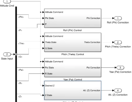
4.1 Position Controller Model

This subsystem implements the control laws for position control of the quadcopter. The subsystem is shown in Figure 4.2. The inputs to this system are the Path command and the State inputs. The outputs from this subsystem is the altitude command which is then sent to the attitude controller subsystem.

(58)

Figure 4.2: Postion Control Subsystem of the Quadcopter

The first block in the subsystem calculates the error feedback using equations 3.5 -3.8. From these PD control laws, error is evaluated, which is then used to develop the position controller for the quadcopter. This subsystem is known as lower level controller, which is used for navigation of the quadcopter in x and y directions. Output from this subsystem is then fed into the higher-level controller for attitude stabilization of the quadcopter.

4.2 Attitude Controller Model

This subsystem implements the control laws for attitude stabilization and control of the quadcopter. The subsystem is shown in Figure 4.3. The inputs to this system are the altitude command from the position controller subsystem and the State inputs

(59)

for the closed loop quadcopter system.

Figure 4.3: Attitude Control Subsystem of the Quadcopter

This subsystem consists of four sub blocks, each of which implements a PID controller using the control laws interpreted in equations 3.1 - 3.4. Each of these sub blocks gives a corrected value of roll, pitch, yaw, and altitude. These values are the outputs from this block which are then sent to the Quadcopter Control Mixing subsystem for further processing. This block completes the controller portion of the quadcopter. These are then used with quadcopter dynamics to navigate and follow the chosen path.

(60)

4.3 Quadcopter Control Mixing Model

Using the output from the attitude stabilization block and mixing equations 4.1 - 4.4, value of the throttle command input is computed. This subsystem is shown in Figure 4.4.

Figure 4.4: Quadcopter Control Mixing Subsystem

Quadcopter Control Mixing block takes the correction values for roll, pitch, yaw, and Z, and then mixes them by letting each correction to be sent to the correct motor accordingly. The equations for the output are

(61)

mc2 =δz−δϕ+δθ, (4.2)

mc3 =δz+δϕ+δφ, (4.3)

mc4 =δz+δϕ−δφ. (4.4)

where mc1−mc4 are percentage throttle command for motors 1-4. Please note that the output of the quadcopter control mixing block is in terms of percent throttle and it allows tuning of the controller, making it a more realistic quadcopter system with properly tuned controller parameters.

4.4 Quadcopter Dynamics Model

In the quadcopter dynamics subsystem, the motor dynamics block restricts the input commands between 0% (minimum) and 100% (maximum) of the throttle. It simulates the motor cutoff behavior at negligible throttle signal and uses the linear relation from equations 4.1 - 4.4 to compute percentage throttle signal considering first order delay function. The output of this block gives the RPM for each motor at any given time. The disturbance block in this subsystem just adds external disturbance effects such as wind forces on the quadcopter for more realistic behavior in simulation. The quadcopter dynamics block is shown in Figures 4.5 and 4.6

Now the heart of the entire simulation where the quadcopter dynamics are modeled.

(62)

Figure 4.5: Quadcopter Dynamics Subsystem

(63)

0 10 20 30 40 50 60 70 80 90 100 Time -1 -0.5 0 0.5 1 1.5 x-Position Motion in x-axis Quadcopter Path

Figure 4.7: Plot of Position Controller Action in x direction

The state equations execute a level 2 S-Function in MATLAB code using all the model dynamic equations as derived in Chapter 2. The output of this subsystem are all the states and outputs, which are fed back making this as a closed loop control for the quadcopter. This quadcopter model with the control method is then validated by moving it through a pre-defined path. The simulation results ofx, y and z positions are shown in Figures 4.7, 4.8, and 4.9 .

(64)

0 10 20 30 40 50 60 70 80 90 100 Time -0.2 0 0.2 0.4 0.6 0.8 1 y-Position Motion in y-axis Quadcopter Path

Figure 4.8: Plot of Position Controller Action in y direction

0 10 20 30 40 50 60 70 80 90 100 Time 0 0.5 1 1.5 2 2.5 3 3.5 4 z-Position Motion in z-axis Quadcopter Path

(65)

(66)

Chapter 5 Vision Based Tracking and

Detection

In this section, we develop and validate the method for tracking the quadcopter using a 2-D image obtained from the camera mounted on the ground vehicle. The camera on the ground vehicle is facing up and forward capturing images of the moving quadcopter above it. The advantage of this setup, where the camera is on the ground vehicle is that the quadcopter can be easily kept in the field of view of the camera. In addition, limits on the data processing and the extra payload due to camera weight are offloaded to the ground vehicle. It is assumed that our quadcopter flies with a known constellation of LEDs or markers. Also, we know the dimensions of our quadcopter. This allows us to easily recover the 3-D pose from a single 2-D frame. The known

(67)

Figure 5.1: Marker constellation of 5 elements arranged on a 3D axis with length of 25 cm for each leg.

constellation of the quadcopter is assumed to be fixed with five elements arranged in a 3-D plane with axis length of 25 cm (arm length of the quadcopter), as shown in the Figure 5.1. Four elements of the constellation are arranged in a plane in the form of a square and the fifth element is set out of the plane. It is this fifth element that helps in resolving the ambiguity between range and yaw for the quadcopter. Also, the 3-D pose estimation problem can also be resolved by tracking with time and, by including the fifth element, it improves the accuracy of the estimation.

Here we have considered a single camera to track the quadcopter. The camera records a two-dimensional image from a three-dimensional scene. Let’s give an outline of the forward model describing the transformations of the five elements from a three-dimensional coordinate system to the two-three-dimensional image coordinate system. In Figure 5.2, the target coordinate system is defined by the pose of the elements on the

(68)

Figure 5.2: Different Coordinate Systems

quadcopter, while the three-dimensional camera coordinate and the two dimensional image coordinate system are defined by the camera orientation.

5.1 Forward Camera Model

Please note that the five marker locations are known and fixed in the target coor-dinate system. The transformation can be described by homogeneous coorcoor-dinates. This simplifies the translational step which is easily reduced to a simple matrix mul-tiplication step. The transformation from locations of the five markers in the target coordinate system to the recorded positions of the markers in the two-dimensional image can be explained by

x=x0f

z0andy =y 0f

(69)

        x0 y0 z0         =         f 0 0 0 0 f 0 0 0 0 1 0             R3x3 T3x1 0 0 0 1                 U V W 1             =P∗R∗C. (5.2)

In the above two equations,x and yare the actual image coordinates and x0, y0 and z0

are the homogeneous image coordinates,P is the projection matrix, Ris the rotation matrix and C expresses the marker coordinates in the target coordinate system. The target coordinate system given by U, V, W are rotated and translated to give the coordinates in three dimensions, with respect to the camera frame of reference. Then it is scaled according to the focal length of the sensor and projected into a two-dimensional image. The coordinates are in two two-dimensional homogeneous coordinates with an offset of z0 overz axis. The homogeneous coordinates are re-scaled such that

z0 = 1.

5.2 Inverse Camera Model

When performing the inverse to get three-dimensional pose from a two-dimensional image, we don’t know thez0 offset value, so we get a non-linear optimization problem.

(70)

The six degree of freedom optimization problem is

[φ, θ, ϕ, Tx, Ty, Tz] =argmin ||pimg−pest(φ, θ, ϕ, Tx, Ty, Tz)||22

(5.3)

where φ, θ and ϕ are the roll, pitch, and yaw of the quadcopter, respectively.

Tx, Ty and Tz are the target translation, pimg is (5 × 2) matrix of the measured

marker coordinates and pest is the estimated marker coordinates in a single frame.

The coordinates of each marker are known for both the target and image coordi-nate system. The values for rotation matrix R3x3 and translation matrix T3x1 are unknown. The rotation matrix R3x3 is characterized by the roll, pitch, and yaw of the quadcopter; therefore, these three angles are sufficient to evaluate the matrix.

5.3 Kalman Filter Tracking

Measurements of the relative position and orientation between the quadcopter and the moving ground vehicle obtained from image processing and estimation are noisy. These measurements along with the noisy signals are used to estimate the target’s position and velocity in the inertial frame.

The single frame pose estimations of the UAV can be combined to form a track of the UAV’s motion over time. By fusing the single frame results and applying a prior

(71)

model for the expected motion characteristics of the platform, we can mitigate errors in the single frame pose estimates. The conventional method for fusing a discrete set of motion measurement is the well-known Kalman filter. As such, the Kalman filer is applied here. A Kalman filter is designed to predict the position of the quadcopter at the next time step. This helps in cases of temporary loss of image or target occlusion. The Kalman filter can be designed considering constant velocity model or constant acceleration model. In this case since the acceleration is assumed to be negligible and velocity of the quadcopter is changing we choose the constant acceleration model. A Kalman filter works in two steps: the prediction step and the update step. In the prediction step, the Kalman filter gives the estimate of the current state variables including uncertainties. Once the next measurement is obtained, the estimates are calculated using a weighted average.

A Kalman filter takes the dynamic model of the system with control inputs and measurements to give an estimate of its state for the next step. It is a recursive estimator and hence for the current state update at time (t) only the estimated state at time (t-1) and measurement at time (t) are needed. For this project, a Kalman filter is implemented for tracking the five marker constellation of the quadcopter. Designing this filter is important and focuses on the following three features to get the best possible tracking

(72)

1. Prediction for location at next time step;

2. Noise reduction caused by inaccurate detections;

3. Proper tagging for multiple objects to their respective tracks.

Before implementing the filter, detecting the five markers from a two-dimensional image is important. For this we simply subtract the Foreground from the image and detect all the circular objects in the image with a specified range for radius. This process is not ideal and hence introduces noise in the detected measurement, but it is simple and efficient. These five marker positions are then used with the inverse model for the camera to get the position and orientation of the quadcopter.

To overcome error in measurement, a discrete Kalman Filter is used. The Kalman filter determines the position whether it is detected in the image or not. This helps if we do not receive a position update or the quadcopter can not be detected in the image. For such scenarios the Kalman filter uses the previous estimate to give a best estimate of the position. So, when the position is estimated the Kalman filter predicts its state and then uses fresh measurements to correct its state and produce a filtered position.

A discrete Kalman filter is formulated as follows. A state vector for target’s position and its orientation to be estimated is defined asx = [XT

t , α]T . The notation ˆxn|m is

(73)

filter is represented by ˆxk|k , the posteriori state estimate, and ˆPk|k, the posteriori

error covariance matrix which gives a measure of the estimate’s accuracy. The two steps for the filter, Predict and Update, are as follows.

vector uk, Hk is the observation matrix, nk is the observation noise assumed to be

zero mean Gaussian noise such that nk ∼ ℵ(0, R), Sk is the innovation covariance

matrix, Kk is the Optimal Kalman gain, and xk|k gives the updated state estimate.

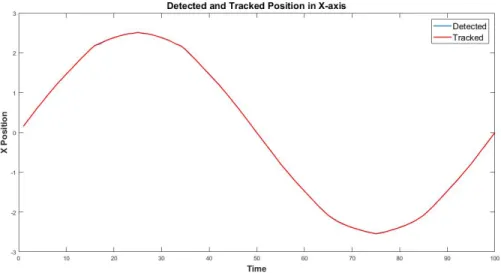
The Kalman filter is implemented on our quadcopter system for tracking. To validate

(74)

Figure 5.3: Detected and tracked position of a quadcopter inx-direction

Figure 5.4: Detected and tracked position of a quadcopter iny-direction

the detection and tracking algorithm we developed a trial run. A simulated video of a randomly moving quadcopter was fed into our algorithm and detection and tracking was implemented for each single frame. The results obtained from this validation are shown in Figure 5.3, 5.4 and 5.5. From these figures, it can be easily inferred

(75)

Figure 5.5: Detected and tracked position of a quadcopter inz-direction

that the detection and tracking algorithm using the Kalman filter works well even with rapidly changing y and z position. The entire simulation also was done with substantial measurement and observation noise. We ran multiple simulations to get an optimum set of parameters to configure our Kalman filter. The error between the tracked and detected position is negligible and our estimation algorithm works efficiently.

(76)

Chapter 6 Closed Loop Feedback with

Ground Vehicle

Now that we have a working position control for our quadcopter, a camera model and an efficient pose estimation algorithm to detect and track the moving quadcopter by using camera inputs only, our next step is to put this algorithm in closed loop feedback architecture with a mobile ground vehicle. In this Chapter we develop a model a moving ground vehicle and then put it in the closed loop system with the quadcopter. The camera is on-board the ground vehicle and the ground vehicle is in motion. One assumption that we make for this closed loop feedback system is that we are in a perfect communication world and the path inputs sent from the ground vehicle reach the quadcopter immediately. First, we design a moving ground vehicle

(77)

and then develop our closed loop feedback system with the quadcopter.

6.1 Moving Ground Vehicle

Several types of ground vehicles have been developed by over the past decades. Ground vehicles can navigate on the ground autonomously or by remote control. These can be deployed to places where human operations are dangerous and inconve-nient. As per its application these can be developed with suitable platform, sensors, controllers, communication links and guidance interface.

The platform for the vehicle is developed according to the terrain in its area of opera-tion. As the primary objective for the vehicle is navigation, several sensors are placed on the platform. These include, but are not limited to, wheel encoders, compasses, gyroscopes, global positioning system (GPS), and cameras. As per requirement, a control system is used for the vehicle to perform decision making process while nav-igating. Communication links and guidance interface are needed to collaborate with other systems and possible remote operation for the ground vehicle. The vehicle takes the sensor inputs and uses the control algorithms to determine next action for a predefined task.

For this problem, we have considered the simplest form of the ground vehicle. Here we

(78)

Figure 6.1: Two Wheel Differential Drive

use a two-wheel differential drive ground vehicle with a pure pursuit control algorithm. A differential drive wheeled vehicle is a drive system which has independent actuators for each wheel; in this case, we have two independent motors for the movement of the vehicle. Both the motors are mounted on a common axis and each can be independently driven clockwise or counter-clockwise for the motion of the vehicle. A two-wheel differential drive vehicle is shown in the Figure 6.1.

For the ground vehicle, it is common to use a two-dimensional planar model. In this part of the thesis, we make use of the forward kinematics of a robot to build a two-wheeled differential drive ground vehicle to be used for the closed loop feedback control of the quadcopter.

(79)

Figure 6.2: Vehicle in an Initial Frame of Reference

velocities of the wheels on the drive to calculate its linear velocity and angular velocity to give position updates for the vehicle at every instant. Figure 6.2 represents the vehicle within an initial frame of reference.

As per the kinematics of this ground vehicle, each of the two motors provide a torque to drive the wheel which is directly proportional to the velocity of the wheel. Since the velocities of the two wheels can be controlled individually, we can drive the ground vehicle to any desired position by making appropriate changes to get the resultant velocity.

In for the kinematic model of the vehicle, we define the state vector for position of the ground vehicle as pg = [xg, yg, βg]T, where xg and yg represent the position of the

center of mass of our two-wheel differential drive vehicle and βg is the orientation

in the body frame. Also, let us define the velocity vector for the ground vehicle as

(80)

Vg = [vg,ωg]T , where vg is the linear velocity for the vehicle and ωg is the angular

velocity for the vehicle at the center of mass. To evaluate the values for velocity vector we use the following equations,

vg =r ω1+ω2 2 , (6.1) ωg =r ω2−ω1 2 . (6.2)

Further, to design the kinematic model governing the motion of the ground vehicle we use the following,

˙ xg =rcos(βg) ω1+ω2 2 , (6.3) ˙ yg =rsin(βg) ω1+ω2 2 , (6.4) ˙ βg =r ω2−ω1 R . (6.5)

where R is the distance between the two wheels, r is the radius of the wheel, and ω1 and ω2 are the angular velocities for each wheel. The value obtained from equation 6.2 for ω is the derivative of the orientationβg of the ground vehicle.

For position update of the moving vehicle in discrete time steps, we have the following,

(81)

yg|t+δt=yg|t+ ˙yg|t∗δt. (6.7)

The above two equations give the updated position, [xg|t+δt, yg|t+δt] at time step of

δt, for the ground vehicle if the position at time t is known to be [xg|t, yg|t]. For our

problem statement, we need to make sure that the vehicle follows the desired path. In short, we need to develop a position controller for this ground vehicle. This can be easily achieved by using a simple PD controller to maintain the orientation of the vehicle which then directly effects the linear velocities, shown in equations 6.3 and 6.4. The following equations are used to control the orientation of the ground vehicle:

u=kpg(βd−βg) +kdg( ˙βd−β˙g), (6.8)

βg|t+δt=u∗δt+βg|t, (6.9)

where kpg and kdg are the PD controller parameters, βd is the desired orientation,

and u is the control input to be applied for update in the present orientation. This algorithm for the position control of the vehicle is known as the pure pursuit to goal algorithm. Using the model described here, the dynamic model of the ground vehicle was developed in MATLAB.

Position Control of an Unmanned Aerial Vehicle From a Mobile Ground Vehicle

Digital Commons @ Michigan Tech

Digital Commons @ Michigan Tech

Position Control of an Unmanned Aerial Vehicle From a Mobile

Position Control of an Unmanned Aerial Vehicle From a Mobile

Ground Vehicle

Ground Vehicle

Dedication

To my family, teachers and friends

Contents

List of Figures

List of Tables

Acknowledgments

Abstract

Chapter 1

Introduction

1.1

Literature Review

1.1.1

Quadcopter Control

1.1.2

Tracking and Vision-Based Estimation

1.1.3

Closed Loop Feedback Control for UAV and ground

vehicle

1.2

Motivation and Research Objective

1.3

Thesis Outline

Chapter 2

Quadcopter Dynamics

Chapter 3

Quadcopter Control

3.1

Attitude Controller

3.2

Position Controller

Chapter 4

Quadcopter Model Developement

4.1

Position Controller Model

4.2

Attitude Controller Model

4.3

Quadcopter Control Mixing Model

4.4

Quadcopter Dynamics Model

Chapter 5

Vision Based Tracking and

Detection

5.1

Forward Camera Model

5.2

Inverse Camera Model

5.3

Kalman Filter Tracking

Chapter 6

Closed Loop Feedback with

Ground Vehicle

6.1

Moving Ground Vehicle