Data-Driven Ghosting using Deep Imitation Learning

(1)

2017 Research Papers Competition

Data-Driven Ghosting using Deep Imitation Learning

Hoang M. Le

1

_{, Peter Carr}

2

_{, Yisong Yue}

1

_{, and Patrick Lucey}

3

California Institute of Technology1_{, Disney Research}2_{, and STATS LLC}3

1. Introduction

Current state-of-the-art sports statistics compare players and teams to league average performance. For example, metrics such as “Wins-above-Replacement” (WAR) in baseball [1], “Expected Point Value” (EPV) in basketball [2] and “Expected Goal Value” (EGV) in soccer [3] and hockey [4] are now commonplace in performance analysis. Such measures allow us to answer the question “how does this player or team compare to the league average?” Even “personalized metrics” which can answer how a “player’s or team’s current performance compares to its expected performance” have been used to better analyze and improve prediction of future outcomes [5].

These measures have enhanced our ability to analyze, compare and value performance in sport. But they are inherently limited because they are tied to a discrete outcome of a specific event. For example, EPV for basketball focuses on estimating the probability of a player making a shot based on the current situation, and is learnt off enormous amounts of historical data. The general use case is then to aggregate these outcomes, and compare and rank them to see how various players and teams compare to each other. In contrast, what we’d really like to know is how teams create time and space for scoring opportunities at the fine-grain level.

With the widespread (and growing) availability of player and ball tracking data comes the potential to quantitatively analyze and compare fine-grain movement patterns. An excellent example of this was the 2013 ESPN article written by Zach Lowe, which described how the Toronto Raptors were using “ghosting” to analyze player decision-making in STATS SportVU tracking data [6]. Specifically, the Raptors created software to predict what a defensive player should have done instead of what they actually did. Developing the computer program required substantial manual annotation, but the insight gained turned heads because it made the effectiveness of defensive positioning both a measurable and viewable quantity for the first time.

Motivated by the original “ghosting” work, we showcase an automatic “data-driven ghosting” method using advanced machine learning methodologies applied to a season’s worth of tracking data from a recent professional league in soccer. An example of our approach is depicted in Figure 1 which illustrates a scoring chance that Fulham (red) created against Swansea (blue). Suppose we are interested in analyzing the defensive movements of Swansea. It might be useful to visualize what the team actually did compared to what a typical team in the league might have done. Using our approach, we are able to generate the defensive motion pattern of the “league average” team, which interestingly results in a similar expected goal value (69.1% for Swansea and 71.8% for the “league average” ghosts -- to fully appreciate the insights revealed by data-driven ghosting, we urge the readers to view the supplemental video at http://www.disneyresearch.com/publication/data-driven-ghosting.)

(2)

Figure 1 Our data-driven ghosting method can be applied to various game contexts to better understand defensive strategies. In the depicted scenario, Fulham (red) scores a goal on Swansea (blue). Ghosts (white) represent where Swansea defenders should have been according to a league average model (LAG) and Manchester City model (MUG).

However in practice, a coach or analyst may not want to compare their defense to the league average, but to another specific team. By “fine-tuning” our league average model to the tracking data from a particular team, our data-driven ghosting technique can estimate how each team might have approached the situation. For example, the coach/analyst may want to see how Manchester City would defend the same attacking play. Using our approach, we can now see how they would defend differently (Figure 1(right)), and how much it changes the EGV (69.1% to 41.7%). The other benefit of using our ghosting approach is that is saves the coach/analyst from searching for similar plays in other matches (which may not even exist).

To achieve automatic ghosting, we leverage a machine learning method called “deep imitation learning”. Our methodology resembles techniques used to teach computers to play Atari [7] and Go [8]. We modify standard recurrent neural network training to consider both instantaneous and future losses, which enables ghosted players to anticipate movements of their teammates and the opposition. More importantly, our approach avoids the need for man-years of manual annotation. Our ghosting model can be trained in several hours, after which it can ghost every play in real-time. In the next sections, we describe the methodology behind our ghosting system, and showcase how automated ghosting can provide insightful analyses and comparisons of team defensive behavior. We also emphasize that our approach is general, and can be applied to a wide range of sports such as basketball and football.

2. Deep Imitation Learning for Modeling Defensive Situations

While the mathematical background required to implement our deep imitation learning method can seem complicated (see Appendix A for full details), the high-level intuition is quite simple. In this section we provide an overview of deep imitation learning, and how it can be applied to soccer tracking data.

(3)

For this paper, we used 100 games of player tracking and event data from a recent professional soccer league. As we are interested in modeling defensive situations, we only focused on sequences of play where the opposition had control of the ball. A defensive sequence is terminated when a goal is scored against the defending team, the ball gets out of the pitch, dead-ball events occur (e.g. foul, off-side), or the defensive team regains possession of the ball. In total, there were approximately 17400 sequences of attacking-defending situations (~3 million frames at 10 frames per second). The average length of all sequences is approximately 170 frames, or 17 seconds.

2.1. What is “Deep Imitation Learning?”

Before explaining what “deep imitation learning” is, we first explain what “imitation learning” is. In many complex situations, it can be very challenging for a human expert to describe and codify the policy or strategy due to the granularity or fidelity of the situation. For such tasks, we can use machine learning to automatically learn a good policy from observed expert behavior, also known as imitation learning or learning from demonstrations, which has proven tremendously useful in control and robotics applications [9-14].

Due to the dynamic, continuous and highly strategic nature of sports like soccer, hand-crafting or manually describing strategy at a fine-grain level is equally problematic. For example in Figure 1, getting a human to describe the location, velocity and acceleration of every player at the frame-level would be prohibitively time-consuming and error-riddled. Even if a human were able to describe the play via rules, it is highly unlikely that another human would be able to learn from such rules as it would surely miss some important context or other information. In practice, a human would just observe many examples until they could understand what to do at a conceptual level. Teaching a computer is no different. The key is to first obtain the right representation which can enable the computer to learn from the observations. In recent years, deep learning has proven to be a powerful tool capable of learning a multi-layer representation hidden in the data, enabling automatic feature discovery that saves tremendous amount of human engineering effort. In this work, we bring together elements from automatic formation discovery [16], imitation learning combined with deep learning methods to learn complex relationships from high-dimensional spatiotempotal sport data domains such as soccer.

2.2. Formation Discovery and Deep Imitation Learning Application

As the data comes from different teams and players, one key component of the pre-processing step is role-alignment (or ordering the players in a form where the computer can quickly compare strategically similar plays). We extract the dominant role for each player from both the defending and attacking team based on the centroid positions throughout the segment of play, regardless of the nominal position of such player. For example, a player whose nominal role is central defender may find himself occupying the dominant role of a midfielder in certain sequence of play. Instead of enforcing a pre-determined formation onto the teams, the centroid positions for

(4)

each sequence are automatically discovered from data by clustering each role, via a linear assignment algorithm, to a role centroid represented by a mixture of Gaussian distributions, in a way that maximizes the self-consistency within role from one segment of play to another (resembles the method from [16]). The result is an average formation across the season closely resembling a 4-4-2 formation.

As soccer is fundamentally a spatial game, one would expect the geometric relationship among players and the ball to contain important semantic and strategic values. We form the full input vector to our model by including not only the absolute coordinates of players and ball, but also the relative polar coordinates (distance and angle) of each player towards the ball, goal, and the role that we try to model. The full feature vector at each time step contains geometric features for all roles in the formation in the form of one mini-block for each role. These mini-blocks are then stacked in a fixed order consistent with role alignment. In order for the model to identify one-on-one versus zone coverage, we also indicate which mini-block of input features correspond to the closest three positions to the role being modeled at each time step. In addition, an extra input vector indicating the team identity is added to the input. This identity vector is useful for learning particular structural and stylistic elements associated with different teams, allowing us the study the impact of tuning our ghosting model to different team styles.

We use recurrent neural networks, a popular deep-learning tool, to learn the fine-grained behavior model for each role in the formation in each time step. A particular type of recurrent neural networks called Long Short-Term Memory (LSTM) was used due to its powerful ability to capture long-range dependencies in sequential data. The model takes in a sequence of input feature vectors as described above and the corresponding sequence of each player’s positions as output labels. Each player is modeled by an LSTM, which consists of two hidden layers of networks with 512 hidden units in each layer. The role of these hidden units is to capture the information from the recent history of actions from all players and map the information to the position of the next time step, in a manner analogous to how an AI program was trained from data to map the history of the game to the next frame of action in Atari and Go.

Using the standard deep learning approach, however, proves insufficient to learn a robust behavior model, due to the typically long temporal span of sequences of play and sheer high-dimensionality of the learning problem. Intuitively, as with any regression method, the model’s predictions can deviate from the groundtruth labels. In sequential modeling settings, this deviation can compound over time and can lead to serious modeling errors. To address this issue, we leverage techniques from imitation learning. The main idea is that we want to train a model that can learn to recover from its own prediction mistakes so that the model can be robust over long sequences of decisions. We use an imitation learning algorithm that learns to capture not only the behavior of each role in the team, but also how multiple players in each team jointly behave from one frame to the next. A full description of our machine learning approach is given in the appendix.

(5)

3. Characterization of The Average Ghosting Team

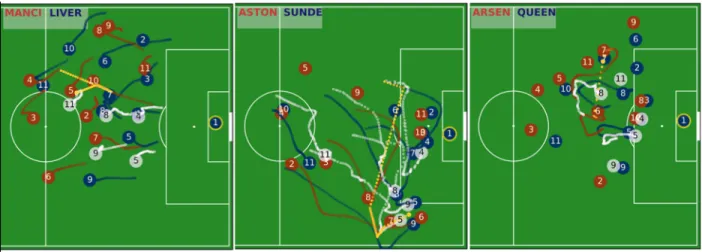
As a first check to see if our league-average model passes the eye-test, we deploy the trained model on held out sequences to inspect whether the trained model behaves in a sensible manner. We observe that our model learned to maintain solid defensive formation and structure, with the modeled players moving in a manner that exhibits spatial and formational awareness. To illustrate this, we show three examples of play in Figure 3.

In the first example, the ghosting players (white) from Liverpool move together with the rest of the teammates (blue) in pressing higher up the pitch in a situation when Manchester City (red) just regained possession in the middle of the field. To avoid clutter, we display only the ghosting trajectories (in white) of the five left positions of the team.

Figure 3 Examples of ghosting behavior for our “league average” model.

Because our algorithm models the interactions between teammates, our ghosted players exhibit high-level coherent team behaviors. In the middle panel of Figure 3, ghost player number 5 of Sunderland broke from formation to challenge the ball carrier number 7 of Aston Villa (red). Ghost player number 9 of Sunderland swaps roles with ghost number 5 and drops back to mark the attacking number 6.

In many situations, the behavior of the “league average” team may be substantially different from the actual play such that the outcome could be different. In the right pane of Figure 3, the ghosting player number 8 more proactively closed the passing lane that could have prevented the shot on goal by attacking number 6 (red), which happened in reality due to the fact that both number 5 and 8 from QPR (blue) drop more deeply and yielded open space.

3.1 Variance from The Average Ghosting by Positions and Team

We can quantify how the players and teams differ from the “average” team. The average level of deviation across all players and teams is about ~4 meters. To put this number in context, note that

(6)

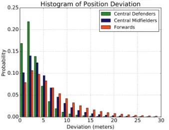
this is a highly accurate average level of precision, as the model has to take into account the arbitrarily long sequence of play. In contrast, more naive machine learning approaches (that do not account for error propagation through time) would suffer from very high levels of prediction error (frequently in the 20-30 meters range). We can further break down the deviation into groups of position. For the defender positions, the majority of the deviations are less than 3 meters apart from the actual player positions. The deviation increases as the dominant positions move further up the field. This reflects increasing level of variation in how attack-oriented players would defend. The defensive behavior of a striker, for example, could change significantly from team to team and among specific players, leading to a higher level of variance by the “average” ghosting positions. We show this deviation according to position in Figure 4.

Figure 4: Deviation from the average ghosting model by positions (Central Defenders (green), Central Midfielders (blue) and Forwards (red)

For our team analysis, we used all 20 teams in our dataset. As we can not disclose the specific performance of these teams, we denote them as teams A-T. At the team level, this variance can indicate which team differs the most from average behavior in terms of defensive positioning. We quantify this out of position ratio by using an 80-20 rule: a player at any given moment is considered out of position if his deviation from his ghost is in excess of the 80th percentile of the entire league average. A breakdown of this tendency gives us a sense of which teams use non-conventional formations. In Figure 5, the teams are sorted by the total number of goals conceded over the season in an increasing order. We analyzed each team’s behavior via two groups: i) “back line” positions (backs), and ii) “front line” positions (midfielders and forwards). While this positioning variance is only one part of the whole picture, note that both the top and bottom teams in the league in terms of the goal conceded were the two outliers. For the top team, the deviation may come in part from the attack-oriented positions (wingers and forwards) exhibiting a wider range of movement relative to other teams. In the case of the bottom team, who ended the season with a relegation, both dominantly defensive and offensive players tend to drift far from the league average.

Figure 5: The out of position frequency (large deviations) by team for both the back and forward positions. Teams are ordered from left to right sorted by the overall goals conceded in the entire season

(7)

3.2 Expected Goal Value of Ghosting Team

A natural use case for ghosting is to study how hypothetical scenarios may unfold, i.e., counterfactual reasoning. In addition to qualitative assessments of ghosting, we also wish to quantitatively assess the effect of alternative defensive reactions to the same situation. As a case study, we analyzed safety-critical play sequences, such as goal scoring opportunities, to see how the play may be altered via ghosting to improve the defensive positioning.

To analyze the goal scoring opportunities, we extracted shot events from the entire season. Concretely, we focussed on the 10-second segments leading up to an open-play shot event, either on or off target (we did not use penalties, free-kicks, set pieces, and game sequences with less than 11 players from either side). We quantified the performance of each model using the Expected Goal Value (EGV) metric [3], which can estimate the goal scoring probability of each shot based on the recent player and ball positions and events. Similar to the setup in Figure 1, for each shot sequence, the average ghost is initialized by the current positions of the defensive players only for the very first frame, and the sequence is unfolded thereafter by running the ghosting model across the remaining time steps. Note that all other factors of the given sequence remained unchanged (attacking player positions and ball movement). At the end of the sequence, the expected goal probability is calculated based on the collective behavior of the ghosting team. The overall EGV is the sum of expected goal

values over all sequences.

The expected performance of the league average team versus the actual outcomes are shown in Table 1. The EGV from open-plays shot events improved compared to the total numbers of goals conceded from all 20 teams (EGV of 474 on actual goal count of 494 from open-plays), primarily due to the “league average” team able to lower the scoring chance against several of the weakest teams in the league (team I, J, K, L and T).

4. Quantifying the Effect of Team Style

Analysts and coaches often want to compare team performance with not just the league average, but also with specific teams and certain characteristics (attack-oriented, possession-based etc.). Doing so at a fine-grained level, however, is difficult and nearly impossible with discrete statistics. Our ghosting system provides a way to not only model the expected trajectory of each player, but also incorporate the ability to impose stylistic elements of specific teams in order to answer the question: how would different teams react to the same situation?

To address this question, we employed techniques from machine learning for domain adaptation. Intuitively, by taking an extra vector indicating the identity of the team as input to the model, our deep-learning based model can extract elements

(8)

relevant to each team’s playing style (such as spatial arrangement, aggressiveness etc.). In any given ghosting scenario, the “average” team model can then be adapted to the playing style of any team in the league by changing the team identity vector, thus allows simulating how the ghost team playing with a different team style would fare under the same scenarios. This is analogous to recent deep learning advances in style transfer, where the stylistic elements from paintings and pictures can be extracted with a data set consisting of, for example, Van Gogh’s works, so that Van Gogh’s painting style can be transferred to other images [15].

We study how different styles can impact the defensive performance, compared to the average model. With domain adaptation, the average model can take on the identities of each of 20 teams in the league, on all 6020 open-play shot events across the entire season. We then compare how the average ghosting team and team-specific ghosts perform relative to the actual outcomes, and to each other.

Figure 6 The effect of assigning different team styles to average ghosting model in terms of total expected goal values over season’s open-play shots (green) vs. total actual number of goals conceded by each team (blue)

Our results are summarized in Figure 6. Interestingly, notice the difference in defensive performance of each team style. Since all other factors are controlled, the difference in overall expected goals conceded can be attributed to different defending styles. We observe a 61.8% correlation between the total EGV coming from different ghosting styles with the overall number of goals conceded in reality. While luck and individual skills matter for any team, team F’s defensive performance seems attributable to an efficient defensive formation (4-5-1 pressing system under a new coach. The formation discovery method of Section 2.2 applied to team F also indicates they frequently play with 5 midfielders, with the variance of midfielders’ movements higher than the rest of the league). During the actual season, team F also possessed the second-lowest goal conceded per open-play opportunity in the league (calculated from Table 1), a statistic consistent with the efficiency of team F’s ghost. Of course, this is only one piece of the defensive equation, since shot events in isolation do not reflect how teams organize their defense long prior to the shot opportunity. In addition, EGV for this type of situation is not perfect, since it does not capture the possibility of defensive ghosts terminating the shot opportunity altogether. Nonetheless, ghosting to different teams in this manner is a still an interesting and novel way to compare defensive behaviors across teams on an equal footing, without relying on disparate statistics coming from different games and scenarios.

(9)

The approach we described thus far is a data-efficient way to extract “personalized” strategic elements from different teams to facilitate both modeling and evaluation. We emphasize that our approach is general and can be applied to modeling not just the average team in the league, but also team-specific models (assuming sufficient tracking data).

5. Example of The Dynamics of Ghosting

Now that we have a better idea of how our ghosting method works, and how the “league average” model varies to a specific team’s model, we can revisit the example shown in Figure 1 and break-down this play in greater detail (a separate video highlighting many different scenarios is available at http://www.disneyresearch.com/publication/data-driven-ghosting).

As before, we consider the sequence of play between Fulham (Red, attacking from left) and Swansea (Blue, defending on right). We compare what Swansea actually did with that of the league average ghosts (LAG - white, top) and the Manchester City ghosts (MCG - white, bottom). The ball trajectories are in yellow. Note that we do not model goal-keeper positions, which are highlighted (number 1). To avoid clutter, we suppress irrelevant trajectories to highlight key players and dynamics.

(10)

The actual scenario resulted in a goal scored against Swansea after a rebound from a counter-attack by Fulham. As mentioned in the previous section, both ghosting models were initialized with the actual positions of Swansea players in the first frame. The ghosting system takes over and makes decision in real-time about how each player should position himself for every frame thereafter. Red#6 and Red#7 open the counter-attack with a “give-and-go pass” to get behind Blue#4 and Blue#7. In stage 1(left column), both LAG and MCG behave similarly as the play unfolds, and closely resemble the actual Swansea defense. The only exception is LAG#8. Compared to Blue#8 and MCG#8, LAG#8 proactively challenges the dribble by Red#6, who in reality drew in Blue#5 and created a wide-open pass to Red#10, leading into stage 2 (middle column). This is the key moment in the play. In the actual sequence, Red#10 is left unmarked and gets an uncontested shot on goalkeeper Blue#1. Here both MCG#5 and LAG#5 positioned themselves further back and were able to get to Red#10 in time to contest the shot. Such attempt hypothetically could have prevented the rebound that led to the goal. As the sequence of events unfold to stage 3, the rebound found Red#9, who is left uncovered by actual Blue#9, leading to the goal (right column). The nuanced difference in positioning by MCG#2 and LAG#2 ended up making a major difference in the scoring chance. Similar to Blue#2, LAG#2 failed to cover Red#9. MCG#2, however, rushed back deeper into the backline from earlier moments of the attack and was in a position to contest the shot on the open net, and could have covered for an attempt by both Red#7 and Red#9. The end result was a reduction in goal probability from ~70% (both actual sequence and LAG sequence) to ~40% by MCG.

The fine-grained simulation and evaluation of defensive scenarios presented here would not have been possible using only discrete statistics as popularly used in sport analytics. Our method is also general and has a rich potential to enable team-specific modeling for both coaching and media analysis purposes.

6. Summary

The ongoing explosion of tracking data has now made it possible to apply powerful modern machine learning techniques to build increasingly fine-grained models of player and team behavior. With

data-driven ghosting, we can now, for the first time, scalably quantify, analyze and compare fine-grained defensive behavior. In this paper, we have demonstrated the value of our approach in a range of case studies. We emphasize that our approach is also applicable to sports beyond soccer, such as basketball and football.

(11)

References

[1] http://www.fangraphs.com/library/misc/war/

[2] D. Cervone, A. D’Amour, L. Bornn and K. Goldsberry, “POINTWISE: Predicting Points and Valuing Decisions in Real Time with NBA Optical Tracking Data” at MIT SSAC, 2014.

[3] P. Lucey, A. Bialkowski, M. Monfort, P. Carr and I. Matthews, “Quality vs Quantity: Improved Shot Prediction in Soccer using Strategic Features from Spatiotemporal Data”, in MIT SSAC, 2015.

[4] B. Macdonald, “An Expected Goals Model for Evaluating NHL Teams and Players”, in MIT SSAC, 2012.

[5] X. Wei, P. Lucey, S. Morgan, M. Reid and S. Sridharan, ““The Thin Edge of the Wedge”: Accurately Predicting Shot Outcomes in Tennis using Style and Context Priors”, in MIT SSAC, 2016.

[6] Z. Lowe. “Lights, Cameras, Revolution”. Grantland. 19 Mar 2013.

[7] R. McMillan. “Google’s AI is Now Smart Enough to Play Atari Like the Pros”. WIRED. 25 Feb 2015. [8] C. Metz. “What the AI Behind AlphaGo Can Teach Us About Being Human”. WIRED. 19 May 2016.

[9] P. Abbeel, and A. Ng. “Apprenticeship learning via inverse reinforcement learning.” In International Conference on Machine Learning (ICML), 2004.

[10] H. Le, A. Kang, Y. Yue and P. Carr, “Smooth Imitation Learning for Online Sequence Prediction”. In International Conference on Machine Learning (ICML), 2016.

[11] B. Argall, S. Chernova, M. Veloso, and B. Browning. “A survey of robot learning from demonstration”. Robotics and autonomous systems, 57 (5):469–483, 2009.

[12] S. Ross and D. Bagnell. “Efficient reductions for imitation learning”. In Conference on Artificial Intelligence and Statistics (AISTATS), 2010.

[13] S. Ross, G. Gordon and A. Bagnell. “A reduction of imitation learning and structured prediction to no-regret online learning”. In Conference on Artificial Intelligence and Statistics (AISTATS), 2011. [14] A. Jain, B. Wojcik and T. Joachims, and A. Saxena. “Learning trajectory preferences for

manipulators via iterative improvement”. In Neural Information Processing Systems (NIPS), 2013. [15] L. Gatys, A. Ecker and M. Bethge. “A neural algorithm of artistic style”. In Neural Information Processing Systems (NIPS), 2015

[16] A. Bialjowski, P. Lucey, P. Carr, Y. Yue, S. Sridharan and I. Matthews. “Large-scale analysis of soccer matches using spatiotemporal tracking data”. In 2014 IEEE International Conference on Data Mining (ICDM), 2014

(12)

Appendix

Data Preparation

Due to the lack of high quality annotated data, we focused on a third of the season worth of matches (~100 games). For the purpose of modeling soccer defense, we further segment the game events into possession sequences. A team is defined to be in a defensive situation when it is not in control of the ball. A defensive sequence is terminated when a goal is scored against the defending team, the ball gets out of the pitch, dead-ball events occur (e.g. foul, off-side), or the defensive team regains possession of the ball after having 2 consecutive touches. This pre-processing step results in approximately 17400 sequences of attacking-defending situations (~3 million frames at 10 frames per second).

One key component of the pre-processing of the data is role-alignment. Role-alignment is necessary for reducing the dimensionality of the learning problem, essentially providing additional context to impose ordering on the training input. At the simplest level, one can view the learning problem as a mapping from the previous positions of 22 players and the ball, to the position of a particular player at the current time step. One key issue with learning this kind of mapping without imposing an ordering is that the data requirement to learn a “permutation-invariant” behavior will need to increase by a factor of billions ((10!)2_{specifically). To reduce this data burden, we first extract the}

dominant role for each player from both the defending and attacking team based on the centroid position throughout the segment of play, regardless of the nominal position of such player. As such, a player whose nominal role is central defender may find himself occupy the dominant role of a midfielder in certain sequence of play. The league average approximates a 4-4-2 formation. In each segment of possession, we order the training data based on the dominant roles, where the

assignment of role attempts to match this average 4-4-2 formation, using the Hungarian algorithm (for minimum cost assignment, where cost measure the distance of each role to each of the 10 possible Gaussian distributions of spatial coverage learned from data).

(13)

As soccer is a spatial game, one would expect the geometric relationship among players and the ball to contain important semantic and strategic values. We form the full input vector for the purpose of training by including not only the absolute coordinates of players and ball, but also the relative polar coordinates of each player towards the ball, goal, and the role that we try to model. Figure 1 describes the structure of a full input vector at each time step. Here the role being model is the left back position. The full input feature vector representing the left back position consist of mini-blocks of features for each role from the defending and attacking team, sorted by a fixed order. The mini-block for the goal-keeper, for example, contains absolute position and velocity, the distance and angle relative to the left-back position, the distance and angle of the goal-keeper to the defending goal, and the distance and angle to the ball at the current time step. In addition to stacking the mini-blocks of features together, we also duplicate the features from the mini-mini-blocks corresponding to the closest 3 positions to the left-back at each time steps. This results in a full input feature of dimension 399 for each role at each frame. We call this input vector the state feature vector for each role.

Deep Multi-agent Imitation Learning

The imitation learning task is to map the state feature vector at each time step to the corresponding action of the player being model, where action is defined as the player position at the following time steps. In principle, this is an online sequence prediction problem, where the model outputs action of a player conditioned on the state of such player, as represented by the recent history of actions of the modeled player, as well as other players. A natural candidate to address such online sequence prediction problem is recurrent neural networks (RNN). A particularly popular class of RNNs, Long Short-Term Memory (LSTM) has been successfully used in recent deep learning applications such as machine translation, speech recognition, handwriting synthesis, etc. Two major differences between our setting and previous applications of LSTM are (i) players need to make decision in real-time, rendering the popular encoder-decoder approach to sequence-to-sequence modeling impractical (ii) our learning set-up belongs to the class of dynamical system learning where action could alter subsequent state distribution, potentially causing a mismatch between training and inference that could severely limit the performance of traditional LSTM models.

(14)

Our proposed method jointly combines training and inference to address both of these issues. This method simulates online prediction in an offline fashion, while allowing the model to gradually learn longer-range prediction. Phase 1 of the algorithm learns a model for each of the 10 roles of the “average” defending team (see figure 9 for an illustration). In phase 2, we used these pre-trained models learned from phase 1 to scale up the training of single player into joint training of multiple players to model collaborative multi-agent learning (figure 10 showcases the joint training of 2 players).

Deep Imitation Learning Algorithm:

To describe our learning algorithm in more details, we generically denote a sequence of state-action pairs as {(s0,a0), (s1,a1),…,(sT,aT)}. We use T=50 in for our ghosting application to soccer defense.

Phase 1: Learn single player model for each role j in {1,2,..,10}

o Initialize a recurrent network model given the ground-truth data set {(s0,a0),

(s1,a1),…,(sT,aT)} for a few iterations

o For k = 1,2,…,T:

▪ For t = 0, k, 2k,.., T:

● For i = 0,1,..,k-1:

o Apply the model to st+i to obtain action a’t+i

o Use the action a’t+i to update the next state st+i+1 (similar to

structure in figure 1 with the new action a’t+i)

● For i = 0,1,…,k-1:

o Use the loss between prediction a’t+i and ground truth action at+i

to update the recurrent network model using stochastic gradient descent

Phase 2: Learn multi player model simultaneously for all role j in {1,2,..,10}

o For k = 1,2,…,T:

▪ For t = 0,k,2k,…,T:

● For i = 0,1,…,k-1:

o Apply the previously trained models for each role j to state vector s(j)t+i to obtain action a’(j)t+i

o Using predicted action a’(j)t+i to update state feature vector for the next time step s(j)t+i+1 for role j and s(j’)t+i+1 for all other role j’

● For i = 0,1,…,k-1:

o Use the loss between prediction a’(j)t+i and ground truth action a(j)t+i to update the recurrent network model for role j using stochastic gradient descent

(15)