Heliostat cost reduction for power tower plants.

(1)

Thesis presented in partial fulfilment of the requirements for the degree of Master of Engineering (Mechanical) in the Faculty of Engineering at

Stellenbosch University

Supervisor: Dr. Jaap Hoffmann by

Arvind Sastry Pidaparthi

(2)

i

Declaration

By submitting this thesis electronically, I declare that the entirety of the work contained therein is my own, original work, that I am the sole author thereof (save to the extent explicitly otherwise stated), that reproduction and publication thereof by Stellenbosch University will not infringe any third party rights and that I have not previously in its entirety or in part submitted it for obtaining any qualification.

Date: March 2017

(3)

ii

Abstract

Heliostats typically contribute to about 40 % of the total installed costs in a concentrated solar power (CSP) tower plant. The objective of this study is to investigate the effects of heliostat size on the levelized cost of electricity (LCOE). These effects are analysed in a power tower with a net capacity of 100 MWe with 8 hours of thermal

energy storage in Upington, South Africa. A large, medium and a small sized heliostat with a total area of 115.56 m2, 43.33 m2 and 16.69 m2 respectively are considered for comparison. The heliostat cost per unit is calculated separately for the three different heliostat sizes and the effects due to size scaling, learning curve benefits and the price index is considered. The annual operation and maintenance (O&M) costs are estimated separately for the three heliostat fields, where the number of personnel required in the field is determined by the number of heliostats in the field. The LCOE values are used as a figure of merit to compare the different heliostat sizes. The lowest theoretical LCOE value of 0.1960 $/kWhe is achieved using the medium size heliostat with an area

(4)

iii

Opsomming

Heliostate dra gemiddeld 40 % by tot die totale geïnstalleerde kostes van ‘n sentrale toring gekonsentreerde sonkrag stasie. Die doel van hierdie studie is om die effek van heliostaat grote op die huidige waarde van die gemiddelde jaarlikse totale koste, [“Levelized Cost of Electricity” (LCOE)] van só ‘n kragstasie te ondersoek. Hierdie effekte word ondersoek op ‘n toring met ‘n kapasiteit van 100 MWe, en 8 ure se

termiese stoor kapasiteit, in Upington, Suid Afrika. ’n Groot, medium en klein heliostaat sal gemodelleer word, met oppervlak areas van 115.56 m2, 43.33 m2 en 16.69 m2 elk, om die resultate te vergelyk. Die heliostaat eenheidskostes word apart bereken vir elk van die drie grotes, met die effekte van opskalering, leer-kurwe voordele en prys-indekse in ag geneem. Die jaarlikse operasionele en onderhoud kostes word vir elke grote apart beraam, waar die hoeveelheid personeel benodig bepaal word deur die hoeveelheid helsiostate in die veld. Die LCOE waardes vir elke grote word gebruik om die meriete daarvan te bepaal. Die laagste teoretiese LCOE wat bereik is, was 0.1960 $/kWhe, vir die 43.33 m2 heliostaat.

(5)

iv

Acknowledgements

I would like to express my sincere gratitude to the following people and organizations: Department of Mechanical Engineering, Stellenbosch University and the Solar Thermal Energy Research Group (STERG) that provided the funding for this research. Dr. J.E. Hoffmann, Senior Lecturer - Department of Mechanical Engineering, Stellenbosch University for his guidance as my supervisor and the freedom he gave me to choose a topic that highly interested me.

Prof. Frank Dinter, Director - Solar Thermal Energy Research Group (STERG) for his support and guidance during my research.

Mr. E.P Dall, with whom I worked very closely and shared ideas about our keen interest in concentrating solar power (CSP) technology and who co-authored a paper with me on CSP performance analysis in SolarPACES 2015.

Researchers from the Helio 100 team (Paul Gauché, Willem Landman and James Larmuth) and STERG for their valuable suggestions.

I would like to thank my family for their love and support – my parents and my brother who always encouraged me to work in the field of renewable energy.

My wife, Manjari, for her love and support during these two years.

My friends at Stellenbosch University, staff at the Department of Mechanical Engineering, the writing lab and Concordia housing.

(6)

v

Dedications

I dedicate this work to my grandfather KVRK Sastry who introduced me to the world of Physics.

(7)

vi

॥ॐध्येयःसदासवित्रमण्डलमध्यिर्तीनारायणसरससजासनसन्ननविष्टः केयूरिानमकरकुण्डलिानककरीटीहारीहहरण्मयिपुरधृर्तशंखचक्रः॥

Always focus your attention at the centre of the solar system, where the sun, the supreme power of the universe, resides.

(8)

vii

List of figures

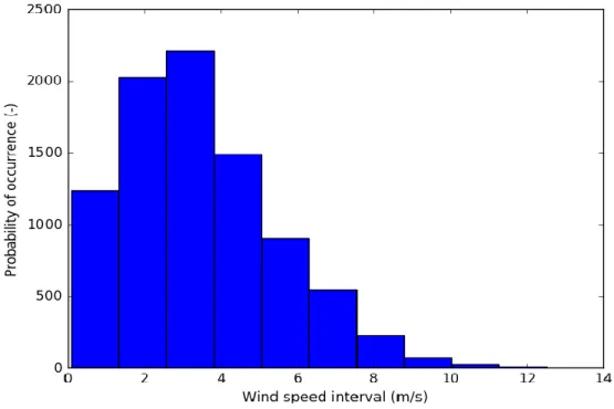
Figure 2.1: Frequency of wind speeds using TMY3 weather data from Meteonorm. .. 8

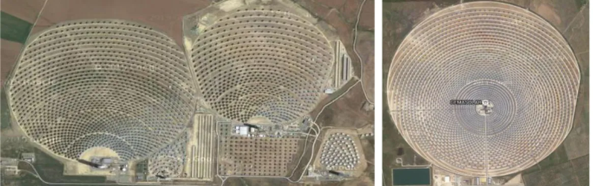
Figure 2.2: A north field used in PS-10 and PS-20 plants (Left) and a surround field used in the Gemasolar plant (Right) (Google Images, 2016). ... 10

Figure 2.3: Radial staggered heliostat field layout where Ris the radial distance and AZ  is the azimuthal distance between the heliostats (Wagner, 2008). ... 11

Figure 2.4: Different towers with their calibration target (Malan, 2014) ... 13

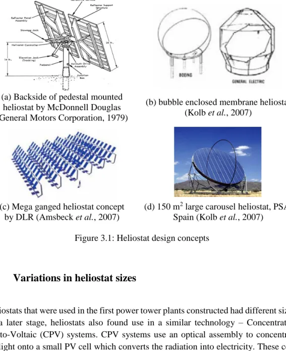
Figure 3.1: Heliostat design concepts ... 19

Figure 3.2: Variations in heliostat sizes offered by eSolar (a) and Abengoa (b) ... 20

Figure 3.3: Historical trend of heliostat sizes (Lovegrove and Stein, 2012) ... 21

Figure 3.4: Heliostat size development in 1980’s (Kolb et al., 2007) ... 22

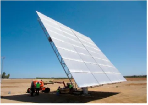
Figure 4.1: A large, medium and a small heliostat considered for this study (Weinrebe, 2014) ... 24

Figure 5.1: Optical losses in a power tower plant (Gertig et al., 2013) ... 31

Figure 5.2: Optical efficiency factors in a power tower (Collado and Guallar, 2013) 32 Figure 5.3: Earth surface co-ordinate system with respect to an observer standing at Q (Stine and Geyer, 2001) ... 33

Figure 5.4: The cosine effect as seen on two heliostats A and B; A is placed in the North and B in the South (Stine and Geyer 2001) ... 38

Figure 5.5: ‘No-blocking’ effect between two heliostats (Wagner, 2015) ... 39

Figure 5.6: Slant distance between the heliostat and the receiver (Lutchman, 2014) 41 Figure 5.7: Representative rectangle used for calculating the spillage efficiency (Lutchman, 2014) ... 44

Figure 6.1: SolarPILOT layout results of a 100 MWe power tower in Upington. ... 47

Figure 6.2: Histogram of beam irradiance in the region excluding zero values ... 50

Figure 6.3: Heliostat geometry (Wagner, 2015) ... 55

Figure 6.4: Slope(left) and specularity errors (right) on a reflected ray (Wendelin, 2003b) ... 58

Figure 6.5: Optimized field layout with 8131 large size heliostats ... 63

Figure 6.6: Optimized field layout with 21 670 medium size heliostats ... 64

Figure 6.7:Optimized field layout with 55 544 small size heliostats ... 64

(13)

xii

List of tables

Table 6.1: Details of plant location in the Northern Cape Province ... 49

Table 6.2: Design point considered for simulation ... 53

Table 6.3: Heliostat geometry design parameters (Weinrebe, 2014) ... 56

Table 6.4: Optimization settings used to generate the heliostat field layout ... 62

Table 6.5: Optimization results for the three heliostat fields ... 62

Table 6.6: Optical performance simulation results for solar noon, spring equinox, 2016 ... 65

Table 6.7: Optical performance simulation results for the three fields ... 66

Table 7.1: Heliostat subcomponent cost for a medium size heliostat (Weinrebe et al., 2014). ... 69

Table 7.2: Solar field maintenance labour ... 76

Table 7.3: Annual O&M costs summary ... 76

(14)

xiii

Nomenclature

A0h Reference heliostat area (m2)

A0rec Reference receiver area (m2)

Aeff Effective reflected image area (m2)

Ah Heliostat total area (m2)

Aineff Ineffective reflected image area (m2)

Al Total land area (m2)

Arec Total surface area of the receiver (m2)

Asf Total reflective area of the heliostat field (m2)

Atotal Total reflected image area (m2)

B Function of day number N (degrees)

Ca Heliostat assembly cost ($)

Cc Heliostat control system cost ($)

Cc,tot Total contingency cost ($)

Cd Heliostat drive cost ($)

Cd,s Subtotal direct cost of the plant ($)

Cd,tot Total direct cost ($)

CEPC,tot Total EPC cost ($)

CF Capacity factor (%)

Cf Heliostat foundation cost ($)

Ch Individual heliostat cost ($)

(15)

xiv

Ch,optic Optical improvement cost per heliostat ($/unit)

Ch,tot Total heliostat field cost ($)

ci Attenuation coefficient with i ranging from 0 to 3 (-)

Ci,tot Total indirect costs of the plant ($)

Cinst,tot Total installed cost ($)

Cl Cost per total land area ($/acre)

Cl,tot Total cost of the land ($)

Cm Heliostat mirror cost ($)

Cnet,cap Total cost per net capacity of the plant ($/kWe)

CP Contingency as a percentage of the total direct costs (%)

CPB Power block cost per electric kilowatt ($/kWe)

CPB,tot Total power block investment cost ($)

Cpiping,c Constant piping loss (kWt)

Cpiping,s Losses that scale with height of the tower (kWt/m)

Cr,ref Reference receiver cost ($)

Cr,tot Total Receiver cost ($)

CRF Capital recovery factor (-)

Cs Heliostat structure cost ($)

Cs Site improvement cost ($/m2)

Cs,tot Total site improvement cost ($)

CSGS Steam generation system cost ($/kWe)

CSGS,tot Total SGS costs ($)

(16)

xv

Ct,fixed Fixed tower cost ($)

Ct,tot Total tower cost ($)

CTES Thermal energy specific ($/kWht)

CTES,tot Total TES system cost ($)

Cw,i Polynomials that scale thermal losses with wind velocity (-)

D Daylight savings (h)

d Slant distance between heliostat and tower (m)

Dhelio Heliostat footprint diameter (m)

Dimage Size of reflected image (m)

DNI Total Annual DNI value (kWh/m2/year)

Drec Receiver diameter (m)

ds Separation distance (m)

Ee,a Annual net electrical energy (kWe)

EOT Equation of time (min)

EPCP EPC costs as a percentage of the total direct costs (%)

Erec Annual energy reaching the receiver (kWt)

f Heliostat aspect ratio (-)

fb Blocking factor (-)

hfc Heat transfer coefficient accounting for forced convection (W/(m2/K))

Hgap Gap length between the panels in the horizontal dimension (m)

Hhelio Heliostat height (m)

hmix Mixed heat transfer coefficient (W/(m2/K))

(17)

xvi

Hrec Receiver height (m)

Ht Tower height (m)

I Intercepted energy (W)

kd Annual debt interest rate (%)

ki Annual insurance rate (%)

krec Receiver cost scaling exponent (-)

kt Tower cost scaling exponent (-)

LC Longitude correction (h)

LCOE Levelized cost of electricity ($/kWhe)

LCT Local clock time (h)

Lv Length of the vertical axis (m)

n Plant lifetime (years)

N Day ‘number’ of the year (-)

N Heliostat normal (-)

n unitized heliostat normal (-)

Nh,TES Number of full load hours of storage (h)

Nhel Total number of heliostats in the field (-)

Npanel,h Number of panels in the horizontal dimension (-)

Npanel,v Number of panels in the vertical dimension (-)

OPEX Annual O&M costs ($)

pi Price index (-)

pr Progress ratio (-)

(18)

xvii

Qdes Receiver design–point thermal rating (MWt)

Qin Incident power (W)

Qloss Heat loss from the receiver system (W)

Qloss,des Design point thermal losses (W)

Qpiping

Piping thermal losses (W)

RGtoN Gross to net conversion factor (-)

s Scaling factor (-)

SM Solar multiple (-)

STB Percentage of total direct costs used to calculate Sales tax (%)

STR Sales tax rate (%)

t scalar parameter of the three dimensional object equations (-) t Unitized target vector (-)

Tamb Ambient temperature (K)

ts Solar time (h)

Twall Average receiver surface temperature (K)

V0

h Reference volume of production as exponent (-)

Vh Current volume of production (-)

vwind Wind velocity (m/s)

Wdes Design turbine gross output (MWe)

Wgap Gap length between the panels in the vertical dimension (m)

Whelio Heliostat width (m)

Wnet Design net output rating of the turbine (MWe)

(19)

xviii

ΔAZ Azimuthal distance between two heliostats in a row (m) ΔR Radial distance between two heliostat rows (m)

Greek alphabet

α Receiver thermal absorptance (-)

αz Solar altitude angle (degrees)

β Slope of the field (degrees)

γs Solar azimuth angle (degrees)

δ Declination angle (degrees)

ε Receiver thermal emittance (-)

εT Elevation angle of the heliostat (degrees) ηa Atmospheric attenuation efficiency (%)

ηb Blocking efficiency (%)

ηc Cosine efficiency (%)

ηdes Cycle thermal efficiency (%)

ηdes Rated cycle conversion efficiency (%)

ηi Image interception/spillage efficiency (%)

ηrec Receiver efficiency (%)

ηs Shading efficiency (%)

ηsf Solar field efficiency (%)

θ Angle of incidence (degrees)

θZ Zenith angle (degrees)

(20)

xix

σast Astigmatic error (mrad)

σbq Beam quality error (mrad)

σgl Gravitational load error (mrad)

σmirror Wind load error (mrad)

σshape Error due to deformations from self loads (mrad)

σslope

Macro slope error (mrad)

σspecular Tracking error (mrad)

σsse Surface slope error (mrad)

σsun Sunshape error (mrad)

σtemp Gravitational load error (mrad)

σtl Temperature load error (mrad)

σtot Effective beam dispersion error (mrad)

σtrack Tracking error (mrad)

σwl Wind load error (mrad)

φ Angle between the receiver and the target vector (degrees)

ϕ Latitude angle (degrees)

ω Hour angle (degrees)

Subscripts i Heliostat number (-) E East (degrees) H Hour number (-) N North (degrees) T Target vector (-)

(21)

xx z Zenith (-) Constants  3.1416  9.3 mrad σ Stefan-Boltzmann constant (5.67 × 10-8 W/m2/K4) Abbreviations

AFD Allowable Flux Density BOP Balance of Plant

CED Cumulative Energy Demand CPV Concentrated Photovoltaic CRF Capital Recovery Factor

CSIRO Commonwealth Scientific and Industrial Research Organisation CSP Concentrated Solar Power

DLR Deutschen Zentrums für Luft - und Raumfahrt DNI Direct Normal Irradiance

EPC Engineering, Procurement and Construction GHG Greenhouse Gas

GIS Geographic Information Systems GUI Graphical User Interface

HAB Heliostat Assembly Building HFLCAL Heliostat Field Layout Calculator HTF Heat Transfer Fluid

(22)

xxi LCOE Levelized Cost of Electricity LFR Linear Fresnel Reflectors MCRT Monte Carlo Ray Tracing

NREL National Renewable Energy Laboratory O&M Operations and Maintenance

PSA Plataforma Solar de Almeria PT Parabolic Trough

PV Photovoltaics PVB Polyvinyl butyral

REIPPPP Renewable Energy Independent Power Producers Procurement Program

RSGS Response Surface Generating System RSS Root Sum Squared

SGS Steam Generating System SNL Sandia National Laboratories

SolarPILOT Solar Power Tower Integrated Layout and Optimization Tool STERG Solar Thermal Energy Research Group

SUNSPOT Stellenbosch University Solar Power Thermodynamic (cycle) TES Thermal Energy Storage

TMY Typical Meteorological Year TOD Time of Day

USA United States of America ZAR South African Rand

(23)

1

1. Introduction

Renewable energy has the potential to supply clean and affordable energy to billions of people across the world. Implementing renewable energy technologies have several advantages which include reduction in pollution levels and creation of new jobs. There are several ways of producing electricity by renewable energy sources, some of which are: Hydro, wind, solar, biomass and tidal energy.

Solar energy can be used for power production, process heat and even cooling applications for the residential and industrial sectors. Solar energy is starting to play a major role in electricity generation and as of early 2016 around 231.8 GW is installed worldwide (REN21, 2016). The solar energy technologies that can be used for power production are solar Photovoltaics (PV) and Concentrated Solar thermal Power (CSP) systems.

PV systems use cells or modules (several cells make up a module) to convert sunlight into direct current. Currently, PV systems are the most widely used solar energy technology for power production and make up for about 227 GW out of the 231.8 GW installed worldwide (REN21, 2016). This is partly due to the fact that these systems can be mounted on the rooftop of a commercial or residential building. PV systems have reached grid parity and are now cost competitive with fossil fuel sources.

CSP systems use mirrors (also called reflectors) with very high reflectivity to concentrate the direct beam radiation (or direct normal irradiance (DNI)) onto a receiver. The radiation is absorbed by the receiver as heat and this heat is transferred to a fluid called heat transfer fluid (HTF) (IRENA, 2013). This heat can be then be used as process heat for various applications or to produce steam in a heat exchanger and generate electricity through steam turbines. CSP tower plants use sun tracking mirrors, also called heliostats, to direct beam radiation onto a central receiver placed on the top of a tower.

This study aims to explore the subject of heliostat cost reduction by investigating the effects of heliostat size on the LCOE for power tower plants. Heliostat cost as a function of size and the optical performance of the heliostat field are included in a holistic LCOE model which compares heliostats of different sizes in a radial staggered

(24)

2

heliostat field layout. Heliostats are often compared on ‘cost per square meter’ basis which does not consider scaling effects, learning curve benefits, subcomponent cost comparison or the optical performance of the heliostat field layout (Larmuth et al., 2016). This study approaches the method of using LCOE as a figure of merit proposed by Weinrebe et al. (2014).

1.1 Background

One of the major engineering challenges faced by engineers working with CSP technology is to effectively concentrate the beam radiation onto the receiver with proper sun tracking techniques (Müller-Steinhagen and Trieb, 2004). This can be achieved by line or point focussing systems. Line focussing systems use rows of parabolic troughs (PT) or linear Fresnel reflectors (LFR) to concentrate the beam radiation onto a stainless steel absorber tube. Special coatings are used on the absorber tube to improve the absorptivity. These systems track the sun in one axis and have low concentration ratios. Concentration ratio is defined as the “the ratio of the area of aperture to the area of the receiver” (Duffie and Beckman, 2013) and higher concentration ratios are desirable for CSP systems. High concentration ratios are indicators of higher operating temperatures and greater precision in tracking the sun. Point focussing systems use curved mirrors mounted on a structure (parabolic dish) or heliostats arranged in a field (power towers or central receivers). Power tower systems have high concentration ratios, thus have the capability to reach very high operating temperatures. Higher operating temperatures lead to higher cycle thermal efficiencies and have a positive effect on the levelized costs of energy (LCOE) (Guédez et al., 2015). Power towers with molten salt as primary HTF can realize temperatures as high as high as 565 °C. Most parabolic trough plants which are currently operational use synthetic oil as HTF and can only operate at a maximum temperature of 393 °C due to temperature limitations of the HTF (Relloso and Lata, 2011). Currently, power tower plants are more capital intensive than parabolic trough plants, due to lower technology maturity and greater land requirements. However, power towers are advantageous since less site preparation is needed and have higher plant efficiencies.

A major advantage with CSP systems is that these plants can be combined with thermal energy storage (TES) systems (Guédez et al., 2015; Helman and Jacobowitz, 2014). This is essential as electricity can be produced after sunset and during peak demand

(25)

3

hours, thereby increasing the capacity factor and the annual energy yield of the plant, which in turn has an effect on the LCOE. The method of calculation of LCOE is widely accepted and used to compare power plants with different technologies on the basis of cost structures and power generation (Kost et al., 2013). Power towers with several hours of TES have the potential to achieve low LCOE values and capacity factors as high as 80 % (Crespo et al., 2012). The high operating temperatures allow for a higher temperature differential, thus reducing the costs of TES (Crespo et al., 2012).

In spite of all these advantages, power towers still face many challenges as they are capital intensive. The major subsystem costs for power towers are: solar collector field, solar receiver, thermal energy storage and power block/balance of plant (Kolb et al., 2011). The heliostat field is one of major cost components of power towers and accounts for about 40 % of the total plant installed costs (Pfahl, 2014). It is therefore very important to reduce heliostat costs to meet the ambitious cost objectives set by the CSP industry of reaching an LCOE of 0.06 $/kWhe by the year 2020 (U.S. Department

of Energy, 2012). This is essential as power towers represent 40 % of the capacity of the CSP plants currently under construction worldwide (REN21, 2015). As of early 2016, the CSP sector has added a total capacity of 4.8 GW worldwide (REN21, 2016) and many more plants are in the construction or development phase. Spain is currently the world leader in terms of the capacity installed with almost 2.3 GW of CSP plants installed (D’Ortigue, 2015). Power towers with a total capacity of 593 MWe have been

built till date and approximately 400 MWe are under construction (ESTELA et al.,

2016).

This study addresses the issue of heliostat cost reduction while evaluating the ‘best suitable heliostat size for a given power tower plant. The hypothetical power tower in consideration is the ESKOM 100 MWe plant (ESKOM, 2016) which is being

considered for Upington, Northern Cape Province (Hoffmann and Madaly, 2015). Heliostat cost reduction for power towers forms a part of research being conducted in the field of renewable energy technology.

1.2 Motivation

The true potential of CSP technology can be estimated when one takes a look at South Africa’s annual DNI values, which are as high as 3000 kWh/m2 in some locations in the Northern Cape (Meyer, 2012). These values are amongst the highest in the world

(26)

4

and are considered ideal for operating power tower plants. A study conducted in 2009 using Geographic Information Systems (GIS) indicates that South Africa has a potential to accommodate CSP plants with a total nominal capacity of 547.5 GW (Fluri, 2009). However, the results of this study only assumed parabolic trough technology installations and did not consider power tower plants. Therefore, it is also important to consider power tower plants in future studies since power towers are much more capital intensive than parabolic trough plants (IRENA, 2016) and need greater land area to build these plants (Ong et al., 2013).

The first power tower plant in South Africa was commissioned in 2016 in Upington, Northern Cape. The plant – Khi solar one – is a direct superheated steam power tower project with a gross capacity of 50 MWe and approximately two hours of steam storage

(Silinga et al., 2015). This plant was developed by Abengoa Solar and has approximately 4120 heliostats, each with an aperture area of 140 m2 (Geyer, 2014). These ‘ASUP 140’ heliostats were introduced by Abengoa in 2012 and are based on the ‘SL 120’ heliostats installed in PS 10 and PS 20 plants in Spain and are expected to lower the costs of the heliostat field by approximately 30 % (Abengoa, 2012). These heliostats will also be used in Abengoa’s 110 MWe Atacama 1 power tower plant in

Chile (Abengoa, 2015).

The second power tower plant in the development phase in South Africa is the Redstone solar thermal power project in Postmasburg, Northern Cape. This plant is being developed by SolarReserve and ACWA Power and is expected to start operations in 2018. The plant will have a gross capacity of 100 MWe with 12 hours of storage and

will generate around 480 000 MWh annually (SolarReserve, 2015). There is no information yet on the heliostats for this plant. SolarReserve’s other power tower plant – Crescent Dunes – in Nevada, USA uses the ‘pathfinder 2’ heliostats, each with an aperture area of 62.5 m2 (Tonopah Solar Energy LLC, 2009) . That plant has a total reflective area of 1 081 250 m² with a total of 17 300 heliostats (Augsburger, 2013). The third power tower in South Africa– Kiwano Solar Power Plant – is in the planning phase with a gross capacity of 100 MWe and is being developed by ESKOM, the

country’s electricity public utility. This plant will have molten salt as HTF and will likely include storage (Hoffmann and Madaly, 2015). The heliostat size has not yet been determined. This study aims to look at the best suitable heliostat size for this plant. The heliostat field is the most expensive component in a power tower system. Therefore reducing these costs is very important for future market development of power tower plants. The configuration of power towers (net capacity not exceeding 150 MWe) in

(27)

5

the planning/development phase in the Renewable Energy Independent Power Producer Procurement Programme (REIPPPP) in South Africa is considered for recommending the optimum heliostat size.

1.3 Objective

The objectives of the study are to:

 Select three heliostats from the three existing defined size ranges, based on the level of commercialization and suitability of implementation in utility scale power towers.

 Review established trends about the heliostat cost-area proportionality for the selected heliostat sizes.

 Develop a mathematical model to include the optical performance of three given heliostat fields and the capital costs of heliostats.

 Optimize the heliostat field layouts to obtain the heliostat positions, receiver dimensions, and tower height and include these parameters in a holistic LCOE model.

 Provide design recommendations, based on the LCOE results, for the best suitable heliostat size for power towers in South Africa with a net capacity of 100 MWe.

1.4 Outline

Chapter 2 describes the location and the design of the power tower plant which sets the scope of the research.

Chapter 3 contains a literature review of the existing research about heliostats in power tower plants, history of heliostat development, variations in heliostat sizes and various heliostat cost reduction studies conducted in the past.

(28)

6

Chapter 4 reviews the heliostat cost as a function of size where heliostats are categorized according to their size. The theory behind the cost-area proportionality used for heliostats is described.

Chapter 5 presents the model developed for the energy performance of the heliostat field where the energy intercepted from the heliostat field is calculated. This involves the precise calculation of the losses in various stages when beam radiation is intercepted at the receiver.

Chapter 6 presents the method in which the heliostat field layout is generated for a 100 MWe power tower with 8 hours of TES and a SMof 1.8. The field is then optimized

and the optimal field layout is then developed. The optical performance simulation results for the heliostat field are then presented.

Chapter 7 presents the economic performance of the power tower configuration. The direct capital costs are calculated with emphasis on heliostat costs developed based on principles observed in Chapter 4. The indirect capital costs and the operations and maintenance (O&M) costs are calculated separately in the cost model.

Chapter 8 combines the thermo-economic performance of the power tower plant and presents the method of calculation of LCOE which is used as a figure of merit for the comparison of the three heliostats chosen for the study.

Chapter 9 presents the results of the study and concludes with the recommendations for future work in this field of research.

(29)

7

2. Plant location and system design

CSP plants utilize only the DNI which is defined as irradiance on the collector perpendicular to the vector from the centre of the sun to the observer and which passes through the atmosphere unaffected (WMO, 2008). There are three major ways to obtain the DNI for a given location: Ground measurements, satellite derived data and to use the combined ground measurements with satellite derived data (Sengupta et al., 2015). Direct ground measurements are given by stations in daily, hourly or sub-hourly intervals and are usually located in areas with high population density, while the locations best suited for CSP plants are either deserts or areas which are very arid and dry (Seidel, 2010). These regions receive a lot of sunlight and since there is significantly less pollution and aerosol density, the direct beam radiation is high (Trieb, 2007). This section describes the plant location in South Africa and design of the power tower plant. The suitable location must have a proper connection to the transmission grid, availability of water and connections via air, railways and roads.

2.1 Site assessment - Solar resource data

The Northern Cape Province in South Africa has attracted several CSP developers as some locations in the province have DNI values as high as 3000 kWh/m2/year (Meyer, 2013). The site chosen for this study is near Upington where a solar park is being considered. The site has a potential for very high solar energy yields combined with good infrastructure needed to build power towers.

A site assessment report was prepared with ground measurements for more than four years and has been compared with satellite derived solar radiation resulting in an enhanced long term DNI average of 2816 kWh/m2/year (Suri, 2011). The terrain is mostly flat hence the site considered for this region is not expected to be affected by any shading. The annual yield of a CSP plant can be calculated in time steps of 60 minutes or interpolated on intervals less than 60 minutes. For this study, hourly values of solar radiation data are used from a typical metrological year (TMY).

(30)

8

2.2 Local conditions and weather data

Local weather conditions like ambient temperature and wind speeds play an important role in the efficiency and annual yield of the whole system. These effects have to be taken into consideration while designing the CSP system. Wind plays a major role in the design of a power tower plant. High wind speeds affect the tracking of the heliostats and lower the accuracy of tracking due to bending and oscillations in the structure (Peterka and Tan, 1987). Higher wind speeds also increase convective losses from the receiver to the atmosphere, thus affecting the first law efficiency of the system. According to Augsburger (2013), wind plays an indirect role in the transient behaviour of the receiver: velocity of a cloud passing over the heliostat field influences the amount of flux reaching the receiver. Fast changes in the flux might cause thermal fatigue or sometimes even failure in the cyclic operation of the receiver and hence its lifetime (Sobin et al., 1976). Figure 2.1 shows a plot of the frequency of occurrence of wind speeds in the region using TMY3 weather data from Meteonorm.

Figure 2.1: Frequency of wind speeds using TMY3 weather data from Meteonorm. Most conventional plants currently use wet cooling technology i.e. evaporation cooling technologies, which require enormous amounts of water in the cooling towers. However it is very common for CSP plants to be planned in areas which are very dry

(31)

9

or arid. Water is usually scarce in these regions, and transporting water to these sites adds to the total expenditure and becomes an important factor. Hence dry cooling technology is considered for this study. The method of dry cooling is governed by dry bulb temperature. The dry bulb temperature, the wet bulb temperature and relative humidity are taken from the same dataset as DNI values.

2.3 Heliostats and the field layout

A heliostat, mounted on a pylon, directs beam radiation onto a receiver located on top of a tower (Stine and Geyer, 2001). Several mounting strategies exist but the most widely used heliostat type is the ‘azimuth-elevation’ concept (Björkman, 2014), which allows the heliostat assembly to move in the azimuth axis, while the elevation axis, which carries the mirrors, is directly above and orthogonal to the azimuth axis (Vant-Hull, 2012). Azimuth-elevation tracking systems use slew drives for the azimuth axis and have high costs. A ‘slope-drive’ axes arrangement using linear actuators for both azimuth and elevation axes are now being considered to save further costs without affecting the performance (Arbes et al., 2016). For this study, the azimuth-elevation configuration is considered for the heliostats. In a given power tower plant, several heliostats are arranged in a collector field in a particular arrangement. These arrangements are reviewed and one arrangement for the heliostat field layout is then chosen.

2.3.1 Heliostat field Layout

Heliostats can be arranged surrounding the tower or on one side of the tower in such a way that there is minimum optical and mechanical interference from one another (Vant-Hull, 2012). A field with heliostats arranged surrounding the tower is called a surround field whereas a field with heliostats on one side of the tower is called a north/polar field. The arrangement of north fields depends on the geographical location of the field. Heliostats are arranged on the north side of the tower in the northern hemisphere while they are on the south of the tower in the southern hemisphere (Falcone, 1986). Several power towers with large capacities of 100 MWe are being built. For such

(32)

10

This is also in agreement with the findings of Yao et al. (2009) that north field configurations are better suited for power towers with small power output capacity. Figure 2.2 shows examples of a north and a surround field.

Figure 2.2: A north field used in PS-10 and PS-20 plants (Left) and a surround field used in the Gemasolar plant (Right) (Google Images, 2016).

There are four types of surround fields mentioned in the literature: Radial staggered, radial cornfield, a random field and phyllotaxis spiral (also called as biomimetic) arrangement (Lutchman, 2014). The radial staggered arrangement has proved to be very efficient in optimizing the field layout using the RCELL and DELSOL codes (Collado and Guallar, 2013). The biomimetic spiral pattern is used to create a layout which imitates a system in nature. For example, heliostats could also be arranged in a phyllotaxis given by the Fermat spiral equations just like florets are arranged on the head of a sunflower. The advantage of using such a layout is that heliostat packing density could be maintained even while moving away from the tower (Vogel, 1979). Of all the layouts presented, recent studies have compared the widely implemented radial staggered layout with the biomimetic spiral pattern. The biomimetic spiral pattern is recommended as the most suitable layout for power towers as this layout is very efficient, maintains high heliostat density thereby requiring lower solar field area (Noone et al., 2012; Zhang et al., 2015a). A study by Ridley (1982) indicates that the normalized packing efficiency of a biomimetic field could be as high as 81 %. However, no plant till date has used this layout. A study on the design methodologies of different heliostat field layout designs and the impact on the power plant efficiencies states that biomimetic algorithms could be an alternative to the radial staggered pattern but concludes that radial staggered layouts offer very close or even better results (Mutuberria et al., 2015). Considering the various points mentioned above, a radial staggered pattern is chosen for this study.

(33)

11

2.3.2 Radial staggered arrangement

The radial staggered arrangement for heliostats was first proposed by the University of Houston (Lipps and Vant-Hull, 1978) and is the most widely and commonly used algorithm for arranging heliostats and requires the least computing resources. This configuration uses two distinctive parameters – the azimuthal spacing between two heliostats in a row and the radial distance between two rows. These two parameters can be represented as a function of the characteristic dimension – the diagonal of the heliostat (Vant-Hull et al., 1991). An additional advantage of using this arrangement is that established codes such as RCELL (Lipps and Vant-Hull, 1978), DELSOL (Kistler, 1986) and SOLERGY (Stoddard et al., 1987) can be used to optimize the heliostat field layout. The tower height, the dimensions of the receiver and the heliostat field layout can be further optimized to get the lowest LCOE values (Sánchez and Romero, 2005). A radial staggered field layout is shown in Figure 2.3.

Figure 2.3: Radial staggered heliostat field layout where Ris the radial distance and

AZ

 is the azimuthal distance between the heliostats (Wagner, 2008).

The radial staggered arrangement for heliostats is optimized using SolarPILOT software where a set of potential positions for each heliostat is generated within the field boundary. SolarPILOT (Wagner and Wendelin, 2016) can be used to generate and optimize heliostat field layouts. The motivation for choosing this software and the modelling approach is described in § 6.1. The optical performance of the heliostat field

(34)

12

layout is evaluated by considering the position of each heliostat individually and estimating its annual performance. Optical efficiency parameters like the cosine, atmospheric attenuation; interception/spillage, blocking, mirror reflectivity and soiling losses are considered during the generation of the heliostat field layout. The radial staggered pattern uses the curve fits where the azimuthal and radial spacing is expressed as follows (Wagner, 2008):

helio L L H R      (1.1442 cot 1.0935 3.0684 2) (2.1) 04902 . 0 02873 . 0 ) 6396 . 0 791 . 1 (        L helio L W AZ   _(2.2) where, t L      2 (2.3)

with _t as the angle between the vertical and the vector from the heliostat to the tower;

helio

H as the height of the heliostat mirror and W_helio as the width of the heliostat mirror. The optimization algorithm and the generation of the field layout is explained in § 6.

2.4 Tower

The primary role of the tower is to hold the receiver. Other important uses of a tower are also to contain a buffer tank for storing the HTF (Augsburger, 2013) and to hold the optical targets (also called as beam characterization targets) below the receiver which is used for periodic calibration of individual heliostats (Malan, 2014). These targets are coated with a white paint and are designed to receive the flux of only one or two heliostats at a time (Stine and Geyer, 2001). The flux density distribution of the reflected beam from the heliostat is then measured for tracking accuracy. Figure 2.4: Different towers with their calibration target (Malan, 2014)Figure 2.4 shows various towers built by power tower developers with their calibration targets enclosed in dotted rectangles.

(35)

13

Figure 2.4: Different towers with their calibration target (Malan, 2014)

The tower also holds the piping system with proper insulation, which is essential to carry the HTF from the top of the tower and back. This ensures that heat losses by conduction from the tower and convection from the pipes to the surroundings are kept to a minimum. The tower must also be designed keeping in mind the costs (costs rise exponentially with the height of the tower); the shadow the tower casts on the heliostat field during operation and the landscape of the surroundings.

Considering the costs to build the tower, it is recommended that towers be made with reinforced concrete if the height of the tower is more than 120 m. A steel lattice tower is recommended when the height of the tower is less than 120 m (Kistler, 1986). The tower is characterized by its height and width and the fixed tower costs. These parameters are optimized using SolarPILOT in this study.

2.5 Receiver

The receiver in a power tower is made up of several panels. Adjacent panels then form passes and each sequential panel in a receiver is in a serpentine pattern (Augsburger et al., 2016). These panels are made up of several vertical tubes which are welded to share a common HTF header The main purpose of the receiver is to convert the concentrated beam radiation into heat which is carried by the HTF flowing in the panels (Augsburger

(36)

14

There are several types of losses during this conversion: reflection of beam radiation from the receiver to the atmosphere, conduction losses, convection losses which depend on the ambient temperature and the wind speeds and radiation losses. Detailed thermal models of the receiver have been developed by Wagner (2008) and very recently using the concept of thermal resistance by de Meyer et al. (2016). The most widely used receivers used are the external cylindrical type or the cavity type and a review of these designs is presented by Ho and Iverson (2014). Since a surround field is chosen for this study, it makes sense to use an external cylindrical receiver.

The receiver is characterized by its height, diameter and the number of panels contained in it. These parameters (along with the aspect ratio and the maximum allowable incident flux) are optimized using the SolarPILOT software for this study.

2.6 TES system

TES systems are employed to shift the excess energy produced during times when solar availability is high to when it is low (Stine and Geyer, 2001). Commercialization of CSP plants with TES systems is now focusing on using molten salt as the heat transfer medium as well as the storage medium. This study assumes a power tower with a molten salt receiver with a ‘two tank’ system. Each tank has the capacity to hold the entire molten salt inventory. According to Helman and Jacobowitz (2014), the thermal storage capacity of the plant represents the total energy that is stored and is expressed in terms of MWht. The thermal capacity is often expressed in terms of the number of

hours a plant can operate directly from storage when running at nominal capacity. A power tower with eight hours of TES in Upington will potentially be able to produce electricity during the peak demand hours from 16:30 to 21:30 in the night. Hence, eight hours of storage is considered.

2.7 Power cycle

The main role of the power cycle is to convert the thermal energy into electrical energy taking the losses into consideration: piping, storage, power cycle and the auxiliary losses (Augsburger, 2013). A power tower plant can be modelled with either a Rankine

(37)

15

cycle or a supercritical carbon dioxide (sCO2) Brayton cycle. Recent research has

shown that sCO2 cycle is an attractive alternative to Rankine cycles for CSP and nuclear

applications due to higher plant efficiencies and higher annual production (Dyreby et al., 2014; Neises and Turchi, 2013). Supercritical carbon dioxide (the fluid state of carbon dioxide) has very high density when it operates near or above its critical point (304.13 K and 7.38 MPa) (Dostal et al., 2004). This high density helps in reducing the size and the power of a compressor, thereby increasing the efficiency of the Brayton cycle and higher power density compared to a Rankine cycle. The sCO2 cycle also

rejects heat at relatively higher temperatures and is advantageous for using heat rejection strategies like dry cooling. This is important since CSP plants are suitable for dry and arid areas where there is a shortage of water.

All the above mentioned characteristics allow for smaller and more compact equipment with higher efficiencies (Iverson et al., 2013; Mehos et al., 2016). However, no power tower plant has yet been built with the sCO2 power cycle. The Rankine cycle remains

the most common and widely used cycle for power towers. With technological advancements, the cycle thermal efficiency (diagram efficiency, excluding parasitic losses) is expected to go up from 42.8 % in 2015 to 43.9 % in 2025 (IRENA, 2016). The operating characteristics of a Rankine power cycle in a conventional power plant do not vary much. On the other hand, the power cycle in a CSP plant must take into consideration the daily and seasonal start-up and shutdown (Hirsch and Feldhoff, 2012), frequent changes in weather – clouds passing over the power plant, and varying HTF temperatures and flow rates (Wagner, 2008). These parameters are important for long term simulations as changes in these parameters affect the performance of the power block. A Rankine power cycle is chosen for this study.

2.8 Conclusion

The techno economic performance of a solar tower is assessed by modelling the conversion of solar radiation to electric power through the major components involved during this process: heliostat field, central receiver system and the power conversion unit (Augsburger, 2013). The heliostat field losses are first calculated: cosine, atmospheric attenuation, interception or spillage, shading and blocking efficiencies respectively. Next, the heat transfer losses from the central receiver tower system are calculated with molten salt as the heat transfer fluid. Finally, the losses due to piping,

(38)

16

storage and other auxiliary equipment are considered for the power conversion unit. The strategy for the plant operation and the design of the heliostat field layout should be modelled using a tariff structure. However, the tariff structure is not incorporated in the model for the generation and optimization of the heliostat field layout. Heliostats are sorted according to the power they deliver to the receiver at each hour. The efficiency of the external cylindrical receiver is calculated and a nominal cycle thermal efficiency is assumed in this study.

The plant operation is simulated on a single design point that is chosen as solar noon on spring equinox similar to a few other studies (Collado, 2009; Kistler, 1986). This point is chosen since the instantaneous power collected at this design point shows very little difference when compared with the annual average power (Collado, 2008a). The optical performance of the heliostat field is included and LCOE is used as the figure of merit to compare heliostats with different sizes.

(39)

17

3. Literature review

This chapter presents a brief overview of the literature reviewed for this study. The role and design considerations of a heliostat in a power tower plant are studied in detail. A short summary of the different heliostat designs developed since the early days of power tower development in the early 1970’s is presented. Focus is then placed on the topic for this research: variation in heliostat size and the different approaches to lower heliostat costs conducted in the past. The method of heliostat design is then summarized with a view of how different components influence the size and cost of a heliostat.

3.1 Heliostats in power tower plants

Each individual heliostat in a collector field has the following components: A reflecting element which is usually a low iron glass mirror; drives; pedestal; foundation; support structures and wiring connections (Stine and Geyer, 2001). Sandwich mirror facets – with a first layer of thin glass mirror (thickness of 0.95 mm), a ‘sandwiched’ layer of polyurethane foam (thickness of around 28 mm) and a steel backward layer (thickness of 0.5 mm) are now being used instead of low iron glass mirrors (thickness of 3~4 mm) (Pfahl et al., 2013). In addition to these components the heliostat field direct costs also include field wiring, labour, installation and transportations costs (Turchi and Heath, 2013).

During the design stage, several issues that must be addressed to maintain high optical efficiency of the heliostat are summarized by Spelling (2012) as follows:

 Reflectivity must be high  Optical precision must be high  Sun tracking must be accurate  Structure must be resistant to loads

In addition to the design considerations mentioned above, wind loads have a radical impact on the costs of heliostats (Björkman, 2014). Hence, both strength and stiffness requirements are taken into consideration while designing heliostats (Blackmon, 2012).

(40)

18

Recent studies also emphasise the importance of carefully selecting the site specific design wind speed to park heliostats to the stow position (Emes et al., 2015; Reeken et al., 2016a) since it was observed that mean wind speeds for different sites differ throughout the year. Environmental aspects like blowing sand, dust and extreme temperatures also affect the design of a heliostat (Blackmon, 2013).

Other requirements like minimal environmental impact impose limits on field preparation and have a direct impact on the foundation of the heliostat. For example, the ‘Ivanpah Solar Energy Generating System’ plant in California had to plan a ‘low impact pylon design’ to allow the sites natural vegetation and contour to remain (BrightSource, 2014). Several countries also have their own codes for structural design and these must be taken into consideration for heliostat support structure design (Blackmon, 2015). For example, recently built CSP plants designed collectors using a design wind speed of 34 m/s in Spain. However, the Eurocodes increased this value to 38 m/s in Spain citing the extreme weather conditions these days. The wind speeds in South Africa are more severe (A collector designed for 40 m/s in South Africa experiences 38 % higher wind loads) than in several countries in Europe with lower design wind speeds (Balz and Reeken, 2015). All these design considerations indicate that heliostat design should take into consideration the geographical location and the environmental conditions of the site.

Several studies were made in the past to investigate methods to reduce heliostat costs; the most recent ones were in 2007, 2011, 2013 and in 2015 ( Kolb et al., 2007, 2011; Coventry and Pye, 2013; Pfahl, 2014; Pfahl et al., 2015). It is therefore necessary to look at the history of development of heliostats including some unconventional designs in the recent past.

3.2 Heliostat development - History

Heliostat development began in the 1970’s, primarily in USA, and continued into the 1980’s. Figure 3.1 shows several design concepts that were developed during this development stage: Pedestal mounted azimuth elevation tracking heliostat in (a), bubble enclosed membrane in (b), ganged Heliostats in (c) and carousel type heliostats in (d). The general trend was to increase the heliostat size to almost 150 m2 to lower the ‘cost per unit area’ which was used as a figure of merit to compare different heliostats. Shortly after the second generation heliostats came out in the early 1980’s,

(41)

19

several other design variables were examined and emphasis was laid on heliostat size optimization.

(a) Backside of pedestal mounted heliostat by McDonnell Douglas (General Motors Corporation, 1979)

(b) bubble enclosed membrane heliostat (Kolb et al., 2007)

(c) Mega ganged heliostat concept by DLR (Amsbeck et al., 2007)

(d) 150 m2 large carousel heliostat, PSA, Spain (Kolb et al., 2007)

Figure 3.1: Heliostat design concepts

3.3 Variations in heliostat sizes

Heliostats that were used in the first power tower plants constructed had different sizes. At a later stage, heliostats also found use in a similar technology – Concentrating Photo-Voltaic (CPV) systems. CPV systems use an optical assembly to concentrate sunlight onto a small PV cell which converts the radiation into electricity. These cells can operate at higher irradiation levels than normal sunlight which is not concentrated (Stoddard et al., 2006). Heliostats developed by Amonix for CPV systems were as large as 320 m2. This trend of favouring larger heliostats is on the basis of the

(42)

20

assumption of several advantages of ‘economies of scale’. For a given heliostat field, larger heliostats have fewer drives, foundations, pedestals and structural assemblies and are easier to operate and maintain when compared with smaller heliostats (Ulmer, 1998).

Heliostats in currently operational power tower plants are in the size range between 1.14 m2, offered by eSolar in 2010, to about 140 m2, developed by Abengoa in 2014. Figure 3.2 shows the variation in size between these two heliostats. Solar field construction costs still remain a huge challenge for large heliostats as they are assembled in a special purpose facility called Heliostat Assembly Building (HAB) (U.S. Department of Energy, 2013). However, the motivation behind eSolar’s small sized heliostats were that they could be constructed and assembled in factories, thus had a huge potential to reduce labour costs on the field (Schell, 2011). eSolar further asserts that their newly developed 2.2 m2 heliostats are still sufficiently small, can be installed manually and do not need a lifting device (Ricklin et al., 2013), further reducing installation costs.

According to Kolb et al. (2007) and as cited by Landman and Gauché (2014), smaller heliostats with higher costs per unit area, but with better optical efficiencies result in the same LCOE values due to the lower tower height, area of the receiver and the number of heliostats. Another advantage with smaller heliostats is that relatively inexpensive linear electric actuators can be used to reduce costs (Buck et al., 2010).

(a) 1.14 m2_{heliostat developed by} eSolar (Google Images)

(b) 140 m2_{heliostat developed by} Abengoa (Google Images) Figure 3.2: Variations in heliostat sizes offered by eSolar (a) and Abengoa (b) It is only very recently that ‘cost versus heliostat size’ has been taken into consideration and there is an indication in literature that the lowest life cycle costs might eventually be achieved by heliostat sizes larger than 50 m2 (Kolb et al., 2011). However, power tower developers and several R&D organizations like NREL, DLR and CSIRO

(43)

21

(Coventry and Pye, 2013) and STERG, are developing very small heliostats, all of which are less than 10 m2_{. Since not many power tower systems have been installed}

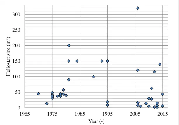
and operated throughout the world, the optimum heliostat size might only be realized when more power tower systems have been installed and operated. Figure 3.3 shows the historical trend in the heliostat sizes and it can be seen that smaller heliostats are also being tested and experimented with since 2007.

Figure 3.3: Historical trend of heliostat sizes (Lovegrove and Stein, 2012) It is difficult to predict the optimum heliostat size for a power tower plant because of the huge variation in the sizes currently available in the market. According to a recent study, heliostats in the size range from 8 m2 _{to beyond 100 m}2 _{were investigated, with}

all applicable costs taken into consideration and an optimum heliostat size of 40 m2 was identified (Bhargav et al., 2013). Another study gives a rough indication that optimum costs are achieved with 16 m2 heliostats for smaller fields and 32 m2 for larger fields. That study is based on the assumption that the maximum facet size is 8 m2 (Pfahl

et al., 2015). 0 50 100 150 200 250 300 1965 1975 1985 1995 2005 2015 He li ostat si ze (m 2) Year (-)

(44)

22

During the early period of heliostat development, costs for electronic parts were relatively high, and larger heliostats were expected to reduce the fixed costs per heliostat. Electronic costs have reduced considerably since then and smaller heliostats are being designed (Lovegrove and Stein, 2012). Figure 3.4 shows the path to developing low cost heliostats that was adopted in 1980’s.

Figure 3.4: Heliostat size development in 1980’s (Kolb et al., 2007)

3.4 Major heliostat cost reduction studies

Several studies, with different approaches, have investigated methods to reduce costs in the heliostat field in a holistic way. These studies are reviewed to get an idea about the different approaches used in the recent past.

A major study on this subject titled ‘Heliostat Cost Reduction Study’ was prepared by Sandia National Laboratories (SNL), USA, in 2007. This report had contributions from approximately 30 heliostat and manufacturing experts from USA, Europe and Australia. The results of this study evaluated the heliostat technology for the year 2006 and gave an estimated price of 126 $/m2_{(based on the material costs and costs of}

(45)

23

deploying labour for ~ 600 MW power towers per year) (Kolb et al., 2007). Further R&D was proposed to ultimately reach a price of 90 $/m2_{. According to this study,}

optimal heliostat size will be more than 50 m2_.

Another study ‘Power Tower Technology Roadmap and Cost Reduction Plan’ also done by Sandia National Laboratories in 2011, indicated that the optimum size of heliostats was difficult to predict and suggested that optimal sizes will only be understood when more power tower systems have been installed. This report also explained that some of the main drivers for both large and small heliostats were drives (27-30 %), manufacturing facilities (23 %) and mirror modules (16-22 %) (Kolb et al., 2011). This study noted that pedestal/mirror support structure and field wiring systems were relatively more expensive for smaller heliostats when compared to larger heliostats because of the number of heliostats.

A heliostat cost reduction survey conducted by Pfahl (2014a) suggests that cost reductions can be realized by decreasing or increasing certain variables in a heliostat sub function. The main heliostat sub functions considered are: reflecting sunlight, fixing shape of reflective material, connecting the system to ground, determining the offset of the mirror plane orientation and turning the reflective material around two axes.

Evaluating the life cycle costs for heliostat sizes, Bhargav et al. (2013) predict that the most promising heliostat size appears to be around 40 m2. The main costs i.e. component, installation and operations/maintenance costs were included while arriving at this conclusion. The method used for this study is to initially consider a small heliostat and ‘scale up’ the size while optimizing for life cycle costs.

According to Coventry and Pye (2013), a few of the promising design concepts are the inclusion of wind fences that reduce both operational and stow condition loads, mirrors or sandwich facets with minimal auxiliary support frames and autonomous heliostats with wireless network communication provided alongside a PV power supply. Unconventional designs like those of Google (Google, 2013) are also reviewed.

(46)

24

4. Heliostat cost as a function of size

This chapter reviews the established trends between the size and the cost of a heliostat. Heliostat size categories are first defined for the small, medium and large heliostats. The importance of heliostat cost scaling relationships is justified as this is central to this study. This chapter also defines the heliostat cost size scaling relationship for the major subcomponent cost categories considered for this study: foundation, metal support structure, drives, controls, reflector panels and assembly.

4.1 Heliostat size categories

Heliostat sizes are categorized into three basic categories: large, medium and small. Large heliostats are assumed to be in the range of 60-150 m2_{, medium heliostats in the}

range of 20-60 m2 and small heliostats in the range of 1-20 m2. These categories do not exist in literature and are defined for the sake of simplicity. Of all the heliostat sizes reviewed, very few heliostats have an area less than 10 m2. However, since 2010 many heliostat developers are developing small heliostats. Figure 4.1 shows the heliostats (large, medium and small) considered for this study.

(a) Large heliostat (b) medium heliostat

(c) small heliostat Figure 4.1: A large, medium and a small heliostat considered for this study

Heliostat cost reduction for power tower plants.

Declaration

Abstract

Opsomming

Acknowledgements

Dedications

Table of contents

List of figures

List of tables

Nomenclature

1.

Introduction

1.1

Background

1.2

Motivation

1.3

Objective

1.4

Outline

2.

Plant location and system design

2.1

Site assessment - Solar resource data

2.2

Local conditions and weather data

2.3

Heliostats and the field layout

2.4

Tower

2.5

Receiver

2.6

TES system

2.7

Power cycle

2.8

Conclusion

3.

Literature review

3.1

Heliostats in power tower plants

3.2

Heliostat development - History

3.3

Variations in heliostat sizes

3.4

Major heliostat cost reduction studies

4.

Heliostat cost as a function of size

4.1

Heliostat size categories