Multiobjective model for optimizing railway infrastructure asset
renewal
Nuno Sousa
Department of Sciences and Technology, Open University, Lisbon, Portugal INESC-Coimbra, Coimbra, Portugal
Luís Alçada-Almeida
Faculty of Economics, University of Coimbra, Coimbra, Portugal INESC-Coimbra, Coimbra, Portugal
João Coutinho-Rodrigues
Department of Civil Engineering, FCTUC, University of Coimbra, Coimbra, Portugal INESC-Coimbra, Coimbra, Portugal
Multiobjective model for optimizing railway infrastructure asset
renewal
A multiobjective model for managing railway infrastructure asset renewal is presented. The model aims at optimizing three objectives, while respecting operational constraints: leveling investment throughout multiple years, minimizing total cost, minimizing work start postponements. Its output is an optimized intervention schedule. The model is based on a case-study from a Portuguese infrastructure management company, who specified the objectives and constraints, and reflects management practice on railway infrastructure. Results show that investment leveling greatly influences the other objectives and that total cost fluctuations may range from insignificant to important, depending on infrastructure condition. The results structure is argued to be general and suggests a practical methodology for analyzing trade-offs and selecting a solution for implementation.
Keywords: rail infrastructure; infrastructure renewal; multiobjective modeling; investment leveling
1. Introduction
Transportation infrastructure is the backbone of a modern economy. Modernizing, and maintaining transportation infrastructure systems requires large investments in order to facilitate the efficient movement of people and goods, promote trade, connect supply chains, and reduce operating costs (BR, 2015).
Railway transportation is environmentally less damaging than other forms of transportation. Powered mainly by electricity, it has a lower carbon profile than all other motorized transportation (Banister and Thurstain-Goodwin, 2011), as well as lower negative externalities than road per unit of activity (Woodburn, 2017). Rail haulage CO2 emissions per tonne-km are seven times lower than road haulage. Rail is also better than road haulage in terms of NOx emissions and particulates (Woodburn and Whiteing, 2015). As such, rail investments are generally perceived as more beneficial
environmentally than other types of transportation investments, and broad consensus exists that rail and its use should be encouraged (Zhang et al., 2018). These advantages caught the attention of the European Commission, which has of late pursued a
restructuring of the European rail transportation market and strengthening of this transportation mode (Menéndez et al., 2016). Three major areas were addressed: (i) opening up to market competition; (ii) improving interoperability and safety of national networks; (iii) developing rail infrastructure. Achieving point (ii) requires railway infrastructure managers to plan and perform maintenance and renewal (M&R)
operations for whole networks to ensure scheduling and safety of daily services (Baldi et al., 2016). Therefore, M&R of railway infrastructure has become increasingly important to avoid system failures and is critical for ensuring safety goals.
In this article, and following mainstream terminology, maintenance and renewal are considered different types of intervention on the infrastructure. Maintenance is taken as an umbrella term for multiple types of intervention (Lee and Wang, 2008). It includes e.g. routine inspections, minor repairs, and preventive and corrective actions, such as tamping or rail grinding. Maintenance actions imply a continuous flow of expenses and preserve service levels. Renewal actions occur at discrete time intervals and reinitialize and/or modernize the infrastructure. Renewal actions involve major overhauls, including replacement of tracks and other assets, larger amounts of resources, and span over lengthier distances and longer periods, thus requiring long-term planning and optimization.
The proposed modeling approach is designed to help infrastructure managers to plan railway assets renewal. It was developed upon request from the Portuguese state-owned company, Infraestruturas de Portugal (IP), which is responsible for maintaining the country’s entire railway network. The approach is multiobjective and incorporates
input from IP, linking methodological research to field practice.
The model addresses three objectives often sought-after by infrastructure managers, namely the even spreading, or leveling of investment peaks over multiple years, minimization of total costs, and minimization of work postponements on higher priority assets. Investment peaks in infrastructure management may appear when maintenance periods align or from budgetary constraints. These may induce
postponements in M&R actions, resulting in accumulation years. When one such peak lies ahead, it may happen that the financial effort required to fully undertake the
necessary repair works in the short-term is too big. A plan is thus necessary to level the investment throughout multiple years. Leveling leads to postponements, which imply rising total costs and requires setting priorities for which assets to repair first, making it necessary to find compromise solutions between the three objectives. Furthermore, operational constraints may affect the works scheduling as e.g. multiple works in the same railway line can cause an unacceptable degradation of customer service. Closing that railway line and carry out all the works simultaneously may be an alternative, but this is very rarely done (Bouch and Roberts, 2010).
This article proposes a modeling approach to find compromise solutions and produce optimized asset renewal schedules, i.e. Gantt charts for the repair works to be undertaken.
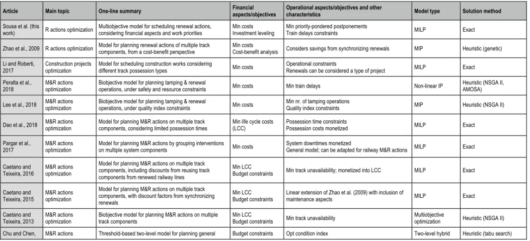
2. Literature Review
The need to cater for rising demand of rail services prompted infrastructure managers to intensify M&R actions, leading various planning problems, often with multiple,
conflicting objectives (see Kabir et al. [2014] and Zavadskas et al. [2018] for a review). Table A1 of Appendix A (see supplemental material) summarizes the state-of-the-art on
M&R planning in railway and related infrastructure, together with a brief summary of the research.
A considerable amount of effort was put in finding optimal ways to decide between, and schedule, infrastructure M&R. General work on the subject include Yoo and Garcia-Diaz (2008), Moghaddam and Usher (2011), Irfan et al. (2012), Zhang and Gao (2012), Chu and Chen (2012), and Pargar et al. (2017). Recently, research on railway-specific M&R actions appeared. One branch concentrated on optimizing synchronized M&R actions on multiple track components, considering track degradation and operational aspects (Andrade and Teixeira, 2011; Caetano and
Teixeira, 2013, 2015, 2016; Dao et al., 2018). Track degradation was also considered by Lee et al. (2018) and Peralta et al. (2018), in tandem with track quality constraints, and safety and resource constraints. Gaudry et al. (2016) pursued finding optimal M&R policies and recurrence periods. Team scheduling aspects were investigated by Pour et al. (2018).
Another branch consisted of optimizing only railway maintenance (M) actions. Pioneering work included the planning model of Higgins (1998), which considered team allocation, works priorities and train delays. Optimization of routine and preventive maintenance was studied by Budai et al. (2006), whereas scheduling of tamping operations was studied by Vale et al. (2012), Gustavsson (2015), Wen et al. (2016), and Khouzani et al. (2017). Other aspects were also considered in the
maintenance-only case, such as e.g. repair team management (Peng et al., 2011; Peng and Ouyang, 2012, 2014), risk and other stochastic aspects, combined with operational aspects (Baldi et al., 2016; Consilvio et al., 2018; Xie et al., 2018).
A different line of research is evaluation of M&R actions, rather than their optimization. Examples include the GIS-based decision support system of Guler (2012), the Markov model of Prescott and Andrews (2015), the Petri networks model of Zhang
et al. (2017), and the multicriteria decision model of Montesinos-Valera et al. (2017). Grimes and Barkan (2006) developed an auditing methodology for railway M&R and used it to evaluate of the outcome of actions by USA infrastructure managers. Odolinski and Wheat (2018) proposed an autoregressive model for the econometric analysis of M&R actions.
This research is complementary to the literature for two reasons. First, it addresses a scenario where all the infrastructure under consideration is overdue for renewal in the short-term. It refers exclusively to renewal (R) actions, aiming at
scheduling these at full network scale. It does not concern maintenance-only actions or choosing between M&R actions. Second, this article introduces investment leveling. To the best knowledge of the authors, this objective was never considered in railway M&R planning. In the reviewed literature financial objectives focused heavily on cost
minimization, in its various forms. Investment leveling was recommended by
IMPROVERAIL (2003, 80) and its importance is bound to rise in times of economic duress. Very little research was done concentrating only on railway renewal actions. A recent example for general infrastructures is the cost-benefit model of Sousa et al. (2017). Railway examples are Zhao et al. (2009), who studied the synergies of combining renewal actions on multiple track components, and Li and Roberti (2017), who investigated scheduling of construction projects, with an emphasis on track possession types. The present research adds to the literature by proposing a
multiobjective model combining investment leveling with financial and operational objectives. It is an original contribution to solve a practical engineering optimization planning problem and a practical management tool, because it is based on requirements from a large-sized infrastructure manager. It is also scalable and adaptable to other infrastructure management contexts.
3. Model
This article uses the terminology of RailNetEurope (2016). In particular “renewal” refers to major repair works following infrastructure wear-and-tear; “line” refers to main railway lines, i.e. intercity and main passenger or freight routes; and “section” to line strips between two geographical reference points (also called “segment”).
Reference points are usually operational points, e.g. junctions or stations, but can also be kilometer marks.
IP has an incoming short-term railway investment peak and requested for an optimization model considering three objectives, namely to level out the peak over five years; minimize total renewal costs; minimize work postponements on the higher priority lines. A railway network is composed of various assets, such as railway lines, stations, powerlines, bridges, etc. The model concerns, by request, renewal of railway line assets (rails/tracks, ballast, sleepers, tie plates, etc.), but can accommodate
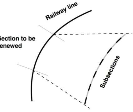
interventions on concomitant assets (bridges, signaling, stations). Renewal operations do not usually require intervening in the full extent of a line; only on sections of it. Each section requiring renewal corresponds to a repair work to carry out. The sections
themselves may consist of several (homogeneous) subsections as depicted in Figure 1. While a work is underway (active), trains cannot circulate at normal speed in the track length under repairs. Speed reduction is necessary, causing circulation delays. Because the infrastructure manager must comply with minimum service requirements, cumulative train delays on a line cannot exceed a certain limit, posing a constraint on the number of repair works simultaneously active in sections of the same line. Also, since lines have different passenger traffic and freight loads, higher priority is given to renewing the busier ones. Repair works on these lines should start earlier.
Figure 1. Railway line, section and segments.
Since spreading renewal actions over multiple years leads to postponing works on some sections, extra maintenance on those sections must be undertaken to ensure minimum safety conditions while renewal is unfinished. This extra maintenance brings additional costs and is the reason total costs are not constant. Two time units are also considered: accountancy time lapse for budgeting investments (year) and time unit for works scheduling. For the latter, the month was considered (by requested), a common time unit in Europe for project planning and contractor payments. Other periods may be considered without affecting the approach. The model is formulated as a mixed-integer linear programming problem (MILP), a common and desirable approach given that problem instances can be solved exactly using highly efficient MILP solvers.
Considering the above and objectives
O1: minimize maximum yearly financial needs O2: minimize total renewal costs
O3: minimize priority-pondered repair works postponements,
the following model is introduced:
Indices:
! = 1, … , & line sections to be renewed.
' = 1, … , ( spanning months.
) = 1, … , * spanning years; ( = 12*.
, = 1, … , - lines. Each section belongs to a line.
Parameters: (units)
./0 cost of renewing section ! (monetary unit).
./123 extra maintenance cost of section ! if not renewed by month ' (monetary unit). Active until the repair works end.
*/ priority for renewing section ! (non-dimensional), i.e. service inconvenience of not renewing the section. Active until repair works end.
4/ time span for renewing section ! (months).
5/ delay to traffic when section ! is under renewal (minutes).
6/7 1 if section ! belongs to line l, 0 otherwise (binary). Note: sections may belong to multiple lines (does not happen in the case-studies).
&7 maximum delay tolerable for line l (minutes).
Decision variables:
8/1 1 if section ! begins renewal in month ', 0 otherwise (binary).
Auxiliary variables:
:/1 1 if section ! is undergoing renewal in month ', 0 otherwise (binary).
;/1 1 if section ! renewal works are not finished as of month ', 0 otherwise (binary). Model: min ?@ = 9 (1) min ?A = B ./0 / + B ./123;/1 /1 (2) min ?D = B */;/1 /1 (3) Subject to: B 8/1 1 = 1, ∀/ (4) 8/1 = 0, ∀/1: ' > ( − 4/ (5) :/1 = B 8/1J 1 1JK1LM NO@,1JP@ , ∀/1 (6) ;/1 = B 8/1J R 1JK1LM NO@,1JP@ , ∀/1 (7) B SB T./ 0 4/ :/1+ ./123;/1U / V @A(XL@)O@A 1K@A(XL@)O@ ≤ 9, ∀X (8) B 5/:/16/7 / ≤ &7 , ∀17 (9)
Explanation/notes:
Eqs. (1) (8): these implement objective O1. The LHS of (8) represents yearly costs for year k (renewal costs and extra maintenance costs). By request, renewal costs for section i are evenly split throughout the months it takes to carry out the works.
Eq. (2): first summation is redundant but was included to give a better grasp of the total cost. Removing it would increase the relative importance of O2. Net present values were not considered due to short project horizons and low inflation rates. Net present values can be considered by adding a time-dependency on renewal costs (./0 →
./10), updating .
/123 values, and adjusting equations (2) and (8) accordingly. This would increase the amplitude of O2 values.
Eq. (3): priority values */ are added monthly to this objective while renewal of section i is unfinished. The higher the priority, the costlier it is (O3-wise) to leave it unfinished. Minimizing the summation means renewing sections with higher */ sooner, thus achieving objective O3. Note that although O2 and O3 both favor starting works as early as possible, they conflict whenever it is necessary to choose between assigning work i1 or i2 to a time slot, where i1 has higher priority/lower EM costs and i2 has lower priority/higher EM costs. Choosing i1 favors O3; choosing i2 favors O2.
Eqs. (4-5): all sections must be repaired and finished before the deadline. Eqs. (6-7): definition of auxiliary variables. ‘A’ stands for ‘active’ and ‘U’ for ‘unfinished’.
Eq. (9): operational constraints preventing excessive delays in train services using line l.
Note 1: by request, extra maintenance costs are accounted for until repair works are fully completed, for technical reasons. A decision maker might want to consider instead lower extra maintenance costs (./123\) while a work is underway, which can be
implemented replacing ./123;
/1 in equations (2) and (8) by ./123];/1− :/1^ + ./123\:/1, with ./123\< .
/123. Another possibility is to consider extra maintenance costs until works reach their half-point, which only requires changing the lower summation on (7) to ' − `MNAa + 1 (the rounding up ensures integer summation indexes for odd 4/). More precise formulations are possible, such as considering extra maintenance costs only for the fraction of a section not yet renewed, but they would require deeper changes to the model and are not expected to be especially relevant to calculation outcomes.
Note 2: by request, the operational constraints (9) focus on delays per railway line. If the transport operator is the same as the infrastructure manager, the integrated company might wish to consider instead delays per passenger train service; and/or delays per freight train service, if these are important in the commercial setup. In this case index l would run through passenger services but constraints (9) would remain the same. Considering delays per railway line and passenger service (and/or freight service) is also possible but requires two sets of constraints (eventually three).
Note 3: maximum delays &7 can be made time-dependent by adding an index j (&7 → &71). This only changes model parameters and allows for more planning
flexibility on months when customer demand is lower. The same goes for priorities (*/ → */1), catering for seasonality in these parameters.
Note 4: closed tracks (blockades) require rerouting of railway traffic or some other field solution. This is however not a big problem for two reasons. First,
infrastructure managers strive to avoid blockades, making them rare (Bouch and
Roberts, 2010). Also, blockade avoidance is possible on two-way lines since traffic can be diverted to one of the tracks while working on the other. For one-way lines, IP and most other infrastructure managers, carry out works during circulation downtime. Second, the model allows incorporating some ways of dealing with blockades, if these
are unavoidable (e.g. switches, catenaries, sub-ballast, law enforced). For instance, for some blockades passengers may be relocated to buses and freight transported by other modes to the next station. This situation is simply a 5/ delay, even though it does not physically correspond to a “train circulating at reduced speed”. If train services absolutely need to be rerouted, the rerouting may congest traffic in the line to which it gets diverted to, leading to delays which can, again, be modeled by 5/. It suffices to set
6/7 = 1 for the diverted-to line to model this situation. More complex formulations are only needed if multiple possibilities for train rerouting need to be considered.
Note 5: besides work priorities (O3), other technical objectives could be considered. An example could be minimization of traffic delays, modeled by min ?b =
c; ∑ 5/ /:/16/7 < c, ∀17, with constraints (9) acting as specific bounds to c. This objective would favor solutions without simultaneous works on the same line, acting against O2 and O3. Other examples would be e.g. minimize disruption duration or duration of breaks between disruptions. These require changes to the modeling
approach and may be considered in future approaches. However, it should be noted that adding objectives increases the complexity of generating and comparing solutions.
4. Case studies
4.1. IP case study
This case study consisted of M = 20 sections, to be renewed over the course of P = 5 years (N = 60 months), making part of Q = 17 lines, and extending over 1000 km, with lengths ranging between 12.6 and 226.8 km and repair times from 6 to 54 months. Parameter values were available per subsection and for sections consisting of multiple subsections, those were aggregated to a single section value through weight-averaging by subsection length (IP recommendation).
Costs
Due to confidentiality agreements, explicit values of renewal and extra
maintenance costs cannot be presented. As such, values of O1 and O2 are presented as relative values, with 100% corresponding to the respective individual optimum. For convenience, the same scale applies to O3.
IP uses a cost model where extra maintenance costs of 3.5% are imposed per each year a renewal is overdue:
./123 = ./fghij(1 + 0.035)(nNL@OX)×p(nNL@OX)− 1q, ∀1∈ year ) (10)
with w/ the number of years section i renewal is overdue when year k arrives, and x(8)
the unit step function, x(0) = 1. The ./fghi are evaluated per km and w
/ can be
negative, meaning renewal will be overdue at some year beyond k = 1. Essentially (10) means that extra maintenance is a 3.5%/year (compound) interest rate on base
maintenance costs. Extra maintenance costs can be modeled in other ways, as ./123 are just fixed parameters. For the IP case-study w/ averaged around 10 years.
Priorities
Three factors were considered for priorities: type of service, conservation status, and maximum freight load. IP defines four types of service (TOS) (suburban, north-south main line, other lines, small branches), four levels of conservation status (CS) (bad, mediocre, reasonable, good), and five levels of freight load (FL) (frequency of cargo trains), with level priority scores of 100/90/75/50 (TOS), 100/90/75/50 (CS), 100/90/75/50/40 (FL). Priority scores were transformed into a single value according to
Both the priority levels, their scores, and weighting factors 0.5/0.3/0.2 of (11) were suggested by IP, but other values are possible, or other priority-setting
mechanisms, such as e.g. multi-attribute utility theory (Keeney and Raiffa, 1993).
Works time span
A reference value of 2.1 km/month per railway track was considered for repair work progress (IP indication). A quarantine time of 0.67 month (20 days) for ballast settlement/consolidation was added to the quotient of section length by progress speed and the result was rounded up to yield 4/. Four railway sections are too long to fit into the N = 60 months total span, so those sections require a double work-front approach, increasing work progress to 4.2 km/month per track, but doubling train delay times and monthly renewal costs.
Delays to train traffic
Circulation speed on sections under intervention is reduced to 30 km/h. Delay (minutes) was calculated on a per-line subsection basis using
5 = ,hÄf 30 − ,hÄf ÅhÄfÇ × 60 + 1 602 ÅhÄf− 30 0.48 × 3.6Ç (12)
where ÅhÄf (km/h) is the normal circulating speed at the subsection and ,hÄf its length (km), truncated to 0.5 km (see below). The first term corresponds to reduced circulation speed and the second to the time spent in breaking/accelerating from ÅhÄf to 30 km/h, assuming uniformly varying motion of 0.48 m/s2 acceleration (reference value). After averaging out subsection values, final values for 5/ were obtained. The reason ,hÄf was truncated is that IP schedules work teams on a weekly basis, so a subsection will not have more than 0.5 km under renewal, the approximate weekly fraction of the monthly progress of 2.1 km. For the sections with double work-front, 5/ was obtained in the above fashion and then doubled. Sections are never geographically contiguous, as they
can be treated as just one larger section in that case.
Maximum line delays
These were fixed by IP according to TOS (maximum 3/4/5/8 minutes delay respectively for the four TOS). For sections consisting of subsections with different TOS, a length-weighted average was carried out and results were rounded up to the next integer minute.
Results
Calculations were carried out using the IBM ILOG CPLEX v12.7 solver, running on an Apple Macintosh i7 3720QM quad-core @2.60 GHz. Initially a pay-off matrix was obtained by minimizing each objective individually (small weights were assigned to the other objectives to ensure obtaining a non-dominated solution).
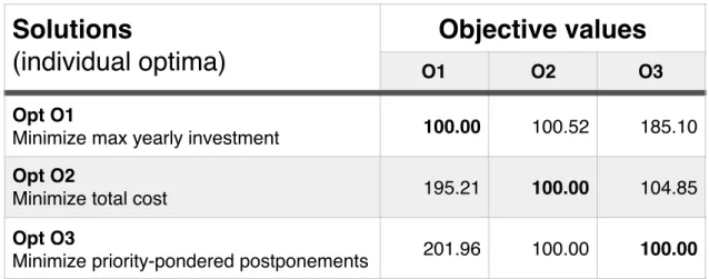
Table 1. Pay-off matrix (individual optima = 100%).
Table 1 shows that optimizing O2 is similar to optimizing O3. This was expected because both objectives aim at starting works as early as possible. The small observed differences are due to the operational constraints, which forbid some repair works to be carried out simultaneously.
Solutions
(individual optima)
Objective values
O1 O2 O3
Opt O1
Minimize max yearly investment 100.00 100.52 185.10 Opt O2
Minimize total cost 195.21 100.00 104.85 Opt O3
Additional non-dominated solutions were obtained using the constraint method (Cohon, 1978). A constraint on the value of O1 was imposed and changed iteratively. For each constrained value of O1, two separate problems were solved, namely
minimizing O2 and O3 (again small weights were assigned to the other objective to ensure obtaining non-dominated solutions). The constraint method was chosen since it can find unsupported, gap solutions, leading to a more complete set of solutions.
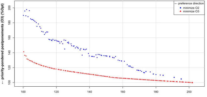
A total of 314 O2/O3-minimizing runs (157 of each kind) was carried out, generating the outcome of Figure 2.
Figure 2. Non-dominated solutions minimizing O2 and O3.
The lower set of solutions (min O3) seems to dominate the upper set (min O2) but both sets consist only of non-dominated solutions, as the upper set has lower O2 values, making it non-dominated. Note also that the upper set is not monotonous
decreasing with O1 because the y-axis is plotting O3 rather than O2. Figures B1 and B2 of Appendix B clarify this point (see supplemental material).
The O2 values (total cost) of all the derived solutions did not vary more than 1% relative to one another. Low values of extra maintenance were the reason for the small
100 120 140 160 180 200 100 120 140 160 180 200
← max yearly investment (O1) (%Opt)
← p ri o ri ty -p o n d er ed p o stp o n em en ts (O 3) (% O p t) ← preference direction minimize O2 minimize O3
O2 variations, reflecting an overall network condition of mild degradation. Since in practice such low level of budget fluctuations is insignificant, the results show that for this particular case study objective O2 can simply be discarded, making the trade-off analysis and solutions comparison easier. Solutions for field implementation should thus be looked for in the lower curve, which has significantly better values of O3.
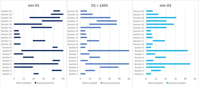
Looking at the trade-offs evidenced by the lower curve of Figure 2, one sees that for an increase of the maximum yearly investment (O1) of circa 150 to 200%, the gain in improving O3 (priority-pondered postponements) is quite small, making this trade-off zone unattractive. On the other hand, reducing O1 from circa 105 to 100% leads to considerable increases of O3. Therefore, it is the O3 zone 105-150% that will probably catch the decision maker’s attention for field implementation. Once a solution is selected, its :/1 values can be used to draw a Gantt chart. Figure 3 shows Gantt charts for three solutions, together with their yearly investment rates (Table 2).
Figure 3. Gantt charts for three solutions.
0 12 24 36 48 60 Section 1 Section 2 Section 3 Section 4 Section 5 Section 6 Section 7 Section 8 Section 9 Section 10 Section 11 Section 12 Section 13 Section 14 Section 15 Section 16 Section 17 Section 18 Section 19 Section 20 min O1
Work schedule Activity (months)
0 12 24 36 48 60 Section 1 Section 2 Section 3 Section 4 Section 5 Section 6 Section 7 Section 8 Section 9 Section 10 Section 11 Section 12 Section 13 Section 14 Section 15 Section 16 Section 17 Section 18 Section 19 Section 20 min O3
Work schedule Activity (months) 0 12 24 36 48 60 Section 1 Section 2 Section 3 Section 4 Section 5 Section 6 Section 7 Section 8 Section 9 Section 10 Section 11 Section 12 Section 13 Section 14 Section 15 Section 16 Section 17 Section 18 Section 19 Section 20 O1 < 120%
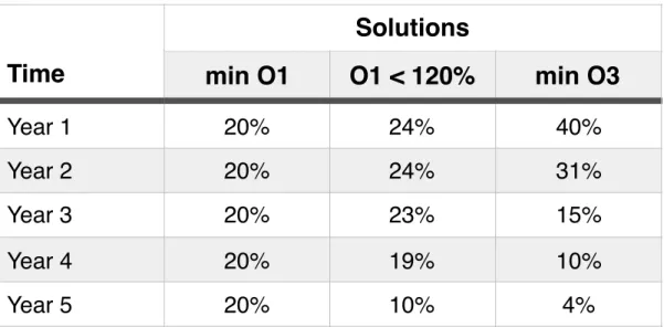
Table 2. Yearly investment rates for three solutions.
As expected, the min O1 solution spreads out repair works through the years to achieve full investment leveling, whereas the min O3 solution clusters repair works into the first years. The O1 < 120% solution comes from the O3-minimizing branch of Figure 2 and shows a compromise schedule. The Gantt charts themselves can also be used to analyze solutions: looking at the work schedules, their geographical locations (maps), and yearly investment values may further assist decision-makers selecting a solution for field implementation, thus complementing the summarized information provided by the objectives’ values.
The trade-offs for this case study are thus clear: the more leveled out yearly investment is, the more some works get postponed, and vice-versa. As to O2, trade-offs in this objective are negligible.
Technical note and CPU times
Only the 8/1 were required to be binary at runtime. Variables :/1 and ;/1 were left as real-valued because constraints (7-8) force them to take binary values. This subtlety removed these auxiliary variables from the branch-and-bound procedure, leading to shorter CPU times. The constraint method was initiated starting from the O1
Solutions
Time
min O1
O1 < 120%
min O3
Year 1
20%
24%
40%
Year 2
20%
24%
31%
Year 3
20%
23%
15%
Year 4
20%
19%
10%
optimum and iterations gradually relaxed this bound. This allowed the solver to retain solutions from the previous run and use them as starting points for the next iteration. This greatly decreased CPU times: the first runs took a few hours to finish, but times subsequently went down to the range of tenths of a second. Despite the large number of
8/1 variables in the model (1200 in total), the model could be solved exactly in reasonable CPU time.
4.2. Large-sized problem
To ascertain whether the model formulation can cope with large instances, and also to know under what circumstances objective O2 becomes important, a large-sized instance was randomly generated, based on the IP case-study, and solved. The instance size was designed to mimic the size of the USA railway network. Since this is the largest
network in the world (Statista, 2018), the authors do not expect considerably larger instances to appear in real life. Results will also reveal interesting properties of the solutions, which hint at a well-defined decision-making strategy.
The instance was generated as follows. Based on the quotient between total railway length of the USA and Portuguese network (circa 89), a total of 1780 sections was considered, belonging to 757 lines. The number of sections per line is roughly double the IP case, which was done to test for a more constrained problem. An average of 25 years renewal overdue was assumed, not only to give O2 more relevance but also to study a scenario of a railway network left to age for decades. Financial unitary costs were the same as the IP case, as were the 3.5%/year extra maintenance costs growth rate. Priorities, train delays, and repair works durations were randomly generated to values similar to the IP case. Finally, given the enormous task of such a large renewal effort, the spanning time was increased from 5 to 10 years. The total of 8/1 binary variables was 213,600.
Results
Runs were carried out as in the IP case-study, restricting O1 from its optimum and relaxing the bound, while optimizing for O2/O3 separately. Then, to study the trade-offs, for each O1 restriction nine extra solutions minimizing a weighted-sum of O2 and O3 were derived, with O2/O3 weights varying from 90/10% to 10/90%, in steps of 10%. This weighted-sum approach was necessary because the alternative of applying the constraint method on two objectives (and optimizing for the third) would make the runs too time-consuming. Weighed-sum runs were not done for the IP case-study because discarding O2 made it unnecessary.
Despite the very large increase in the number of decision variables, the CPU time increase was not significant, with most individual runs taking in the range of minutes and runs close to O1 optimum again taking a few hours, a reasonable increase for a problem that is almost 200 times as large, and more constrained. It is thus
expectable that any real problems can be treated in a modern computer, regardless of size. For both case studies, the time scales for obtaining results using the exact methods proposed in this article are quite acceptable for a long-term planning problem, so there is no need to resort to other solution-seeking methods such as meta-heuristics or specialized heuristics.
Table 3 shows the pay-off matrix for this large-sized instance. As compared to the IP case, optimizing O1 now leads to greater degradation of O2 and O3.
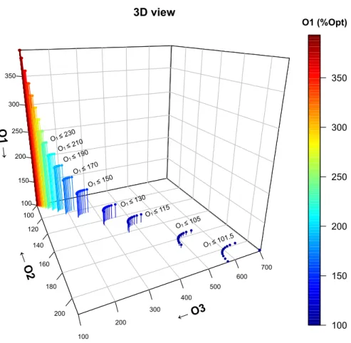
Because in this case O2 becomes important, the non-dominated solutions shown in Figure 4.1 were plotted 3D.
Table 3. Pay-off matrix for the large-sized instance (individual optima = 100%).
Figure 4.1. Results for the large-sized instance in 3D plot.
Solutions
(individual optima)
Objective values
O1 O2 O3
Opt O1
Minimize max yearly investment 100.00 210.14 703.31
Opt O2
Minimize total cost 393.71 100.00 102.87
Opt O3
Minimize priority-pondered postponements 392.47 100.26 100.00
← O2 100 120 140 160 180 200 ← O3 100 200 300 400 500 600 700 O1 → 100 150 200 250 300 350 3D view 100 150 200 250 300 350 O1 (%Opt) O1 ≤ 101.5 O1 ≤ 105 O1 ≤ 115 O1 ≤ 130 O1 ≤ 150 O1 ≤ 170 O1 ≤ 190 O1 ≤ 210 O1 ≤ 230
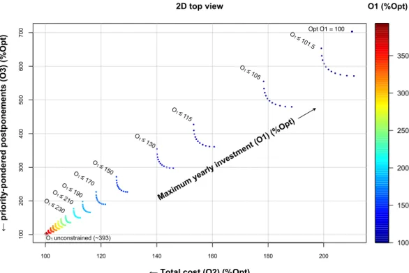
Figure 4.2. Results for the large-sized instance in O2/O3 xy plot.
Contrary to the IP case, objective O2 is now relevant, showing all objectives are important when the backlog is large. If the decision maker wants to have a good
leveling of yearly investment, close to 10%/year, total costs almost double. The extra maintenance costs and increase of work span to 10 years are the reasons this happens, so clearly when the railway infrastructure is very degraded, well past its lifetime, O2 cannot be neglected in the analysis, especially if the renewal project spans for many years. Allowing some increase in max yearly investment (degradation of O1), solutions improve considerably in the other objectives: raising O1 to 130%, total costs (O2) drop from 210% to 140-145% while, simultaneously, priority delays (O3) drop from 700% to 300-350%. At this point solutions start to appear where no investment is done in the final years, making it possible to finish the project before the deadline. Relaxing O1 further makes solutions start to cluster around each other and become globally similar.
100 120 140 160 180 200 100 200 300 400 500 600 700 2D top view
← Total cost (O2) (%Opt)
← p ri o ri ty -p o n d er ed p o stp o n em en ts (O 3) (% O p t) 100 150 200 250 300 350 O1 ≤ 130 O1 ≤ 150 Opt O1 = 100 O1 unconstrained (~393) O1 ≤ 105 Maxim um ye arly in vestm ent (O 1) (% Opt) O1 ≤ 115 O1 ≤ 101.5 O1 (%Opt) O1 ≤ 170 O1 ≤ 190 O1 ≤ 210 O1 ≤ 230
For each bound on O1, figure 4.2 shows that O2 and O3 can only fluctuate in a narrow range of values, making O1 a very important objective, whose value has a big influence on the two other. This phenomenon is expected to be general, since both O2 and O3 minimize under similar conditions making it plausible that Pareto fronts for any instance will tend to look like Figure 4.1. The data can increase or decrease O2/O3 fluctuation amplitudes: if the works with higher priority correlate positively with the most expensive ones (in terms of extra maintenance costs), solutions minimizing O2 or O3 will be more similar, leading to narrower fluctuations. If that correlation is negative, the opposite occurs.
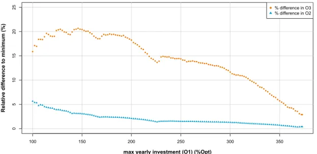
Figure 5 gives a break-down of the relative size of these fluctuations.
Figure 5. O2 and O3 fluctuations for each O1 restriction.
The O2 fluctuations become small (< 4%) for O1 values in mid-to-high range (e.g. O1 > 140%) so the decision-maker may opt for selecting O3-minimizing solutions, given its fluctuations are more significant than those of O2, in this O1 range. If O1 is instead at low values (< 140%), O2 starts to vary more (4-6%), in which case the
decision maker might consider one of the O2/O3 weighted-sum minimizing solutions of
100 150 200 250 300 350 0 5 10 15 20 25
max yearly investment (O1) (%Opt)
R el ati ve d iffe re n ce to m in im u m (% ) % difference in O3 % difference in O2
Figure 4.2. In deriving weighted-sum solutions it is preferable to use a difference-ratio normalization scheme for the weights, such as e.g.,
Ü/R = Ü/
max ?/ − min ?/ (13)
where Ü/R and Ü
/ are respectively the normalized and un-normalized weights, and
max ?/ and min ?/ are the max/min values of O2 and O3 in the O1-restricted
subproblem (index i refers to O2/O3). Other normalization schemes were tried but in practice they tend to skew solutions towards the regions near O2/O3 optima.
Summarizing the trade-offs for this large-sized instance, one sees that achieving good values of investment leveling (O1) has a large impact on the other objectives (O2/O3), degrading them more than in the IP case. Moving just 15-30% away from the O1 optimum leads to considerable improvements to O2/O3. It is natural to consider O1 before attending to O2/O3, as the trade-offs between O2 and O3 are milder after O1 is set.
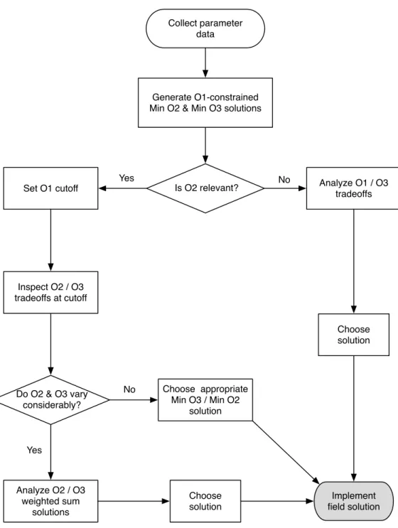
4.3. The decision-making process
Based on the results derived and the considerations they led to, a methodology for the decision-making process based on the modeling approach can be proposed.
The first step is to generate and plot two sets of solutions with restricted O1 that minimize O2/O3 respectively, gradually relaxing the restriction from O1 optimum up to unconstrained. This enables the decision maker to have an overall view at the pay-off between objectives and realize whether O2 is relevant. If O2 fluctuations are small enough to be deemed irrelevant (e.g. IP case-study) the decision-maker only needs to analyze the O1/O3 trade-offs and select a solution for field implementation.
If, however O2 cannot be discarded, the decision-maker may, on a second step, put a cut-off value on O1 such that O2 (or O3, for that matter) does not rise above an
acceptable total cost (or priority postponements), and explore the solution space near this cut-off.
The third step is to check whether the trade-offs between O2/O3 in the solutions minimizing O2/O3 near the cut-off happen to vary considerably. If one of these
objectives has a low variation (e.g. < 5%), the solution minimizing the other objective is an excellent candidate for field implementation.
If, however both show significant variation, the final, fourth step, is deriving weighted-sum solutions at the cut-off point and finally selecting one of those for field implementation.
The flowchart of Figure 6 summarizes the proposed methodology for decision-making.
This methodology reflects the solutions structure of the model and is expected to be general. Its simplicity makes it a useful tool for decision-makers, as multiobjective optimization problems typically have many efficient solutions, whose trade-offs are often hard to analyze. The proposed modeling approach hints instead at a clear strategy for navigating through the maze of alternative solutions, even for non-experts. Authors are therefore firmly convinced it is of practical value, with good potential to be used by infrastructure management companies.
Figure 6. Decision-making process for the modeling approach.
4.4. Applications to other infrastructure renewal situations
Other transportation infrastructure systems bear similarities to railways and hence call for similar management decisions. One such example is road infrastructure, where
Analyze O1 / O3 tradeoffs
Do O2 & O3 vary considerably?
Generate O1-constrained Min O2 & Min O3 solutions
Set O1 cutoff Inspect O2 / O3 tradeoffs at cutoff Is O2 relevant? Analyze O2 / O3 weighted sum solutions Choose appropriate Min O3 / Min O2 solution Yes Choose solution Choose solution No Yes No Implement field solution Collect parameter data
limits in annual budgets of highway agencies for rehabilitation projects may result in large backlogs for M&R works. For the particular case of renewal actions, once a given number of road sections are marked for this type of intervention, the model presented in this article can then be used to schedule those interventions. If so, the model remains the same, but parameter evaluation becomes rather different. Also, train delays become road traffic delays, and congestion issues might need to be considered. The operational constraints (9) may remain the same, as the problem can only be constrained by the impossibility of executing multiple works on the same road. Given the overall bad condition of the USA road infrastructure (ASCE, 2017), the proposed modeling approach might prove to be more valuable for this case than for the railway one, especially since the degradation rate of roads is typically higher than that of railways, increasing the importance of O2.
5. Conclusions and summary
In this research, a model to address the real-life asset management problem of planning large scale railway infrastructure renewal actions was presented. The proposed model considers three management objectives, namely minimizing maximum yearly
investment (investment leveling); minimizing total cost; minimizing postponements in the higher priority works, while attending to operational constraints which guarantee that passenger and freight services are not excessively delayed from having railway line sections under renewal. The model is linear and can produce exact non-dominated solutions in reasonable time, even for large-sized instances. Its solutions structure naturally suggests a methodology to analyze trade-offs between objectives, making it simpler to select one solution for field implementation. As such, authors believe it is a valuable and practical new tool in planning for large scale railway infrastructure renewal actions, thus helping to foster the choice for this sustainable, low-emissions
transportation mode. It is also general enough to be applied to other transportation infrastructure asset management problems.
Acknowledgements
This work was partially supported by the Portuguese Foundation for Science and Technology under project grant UID/MULTI/00308/2013.
References
Andrade, A., and P. Teixeira P. 2011. “Biobjective Optimization Model for Maintenance and Renewal Decisions Related to Rail Track Geometry.” Transportation Research Record 2261:163-170. doi:10.3141/2261-19
ASCE – American Society of Civil Engineers. 2017. 2017 Infrastructure Report Card. ASCE Foundation. http://www.infrastructurereportcard.org
Baldi, M., F. Heinicke, A. Simroth, and R. Tadei. 2016. “New heuristics for the Stochastic Tactical Railway Maintenance Problem.” Omega 63:94-102.
doi:10.1016/j.omega.2015.10.005
Banister, D., and M. Thurstain-Goodwin. 2011. “Quantification of the non-transport benefits resulting from rail investment.” Journal of Transport Geography 19(2):212-223. doi:10.1016/j.jtrangeo.2010.05.001
Bouch, C.J., and C. Roberts. 2010. “State of the art for European track
maintenance and renewal logistics.” Journal of Rail and Rapid Transit 224(4):319-326. doi:10.1243/09544097JRRT315
BR – Business Roundtable. 2015. Road to Growth: The Case for Investing in America’s Transportation Infrastructure. Business Roundtable.
https://s3.amazonaws.com/brt.org/archive/2015.09.16%20Infrastructure%20Report%20 -%20Final.pdf
Budai, G., D. Huisman, and R. Dekker. 2006. “Scheduling Preventive Railway Maintenance Activities.” Journal of the Operational Research Society 57(9):1035-1044. http://www.jstor.org/stable/4102318
Caetano, L., and P. Teixeira. 2013. “Availability Approach to Optimizing Railway Track Renewal Operations.” Journal of Transportation Engineering 139(9):941-948. doi:10.1061/(ASCE)TE.1943-5436.0000575
Caetano, L., and P. Teixeira. 2015. “Optimisation model to schedule railway track renewal operations: a life-cycle cost approach.” Structure and Infrastructure Engineering 11(11):1524-1536. doi:10.1080/15732479.2014.982133
Caetano, L., and P. Teixeira. .2016. “Strategic Model to Optimize Railway-Track Renewal Operations at a Network Level.” Journal of Infrastructure Systems 22(2). doi:10.1061/(ASCE)IS.1943-555X.0000292
Chu, J., and Y.-J. Chen. 2012. “Optimal threshold-based network-level transportation infrastructure life-cycle management with heterogeneous maintenance actions.” Transportation Research Part B: Methodological 46(9):1123-1143.
doi:10.1016/j.trb.2012.05.002
Cohon, J. 1978. Multiobjective Programming and Planning. New York: Academic Press. ISBN:0121783502.
Consilvio, A., A. Di Febbraro, R. Meo, and N. Sacco. 2018. “Risk-based optimal scheduling of maintenance activities in a railway network.” EURO Journal on Transportation and Logistics (in press). doi:10.1007/s13676-018-0117-z
Dao, C., R. Basten, and A. Hartmann. 2018. “Maintenance Scheduling for Railway Tracks under Limited Possession Time.” Journal of Transportation Engineering, Part A: Systems 144(8). doi:10.1061/JTEPBS.0000163
Gaudry, M., B. Lapeyre, and E. Quinet. 2016. “Infrastructure maintenance, regeneration and service quality economics: A rail example.” Transportation Research Part B: Methodological 86:181-210. doi:10.1016/j.trb.2016.01.015
Grimes, G.A., and C.P.L. Barkan. 2006. “Cost-Effectiveness of Railway Infrastructure Renewal Maintenance.” Journal of Transportation Engineering 132(8). doi:10.1061/(ASCE)0733-947X(2006)132:8(601)
Guler, H. 2012. “Geographic information system-based railway maintenance and renewal system.” Proceedings of the ICE – Transport 165(4):289-302.
doi:10.1680/tran.10.00067
Gustavsson, E. 2015. “Scheduling tamping operations on railway tracks using mixed integer linear programming.” EURO Journal on Transportation and Logistics 4(1):97-112. doi:10.1007/s13676-014-0067-z
Higgins, A. 1998. “Scheduling of Railway Track Maintenance Activities and Crews.” Journal of the Operational Research Society 49(10):1026-1033.
http://www.jstor.org/stable/3010526
Irfan, M., M.B. Khurshid, Q. Bai, S. Labi, and T.L. Morin. 2012. “Establishing optimal project-level strategies for pavement maintenance and rehabilitation – A framework and case study.” Engineering Optimization 44(5):565–589.
doi:10.1080/0305215X.2011.588226
IMPROVERAIL. 2003. Deliverable 10: Project Handbook. IMPROVEd Tools for RAILway Capacity and Access Management. Report.
http://www.transport-research.info/sites/default/files/project/documents/20060727_145926_44007_IMPROV ERAIL_Final_Report.pdf
Kabir, G., R. Sadiq, and S. Tesfamariam. 2014. “A review of multi-criteria decision-making methods for infrastructure management.” Structure and Infrastructure
Engineering: Maintenance, Management, Life-Cycle Design and Performance 10(9):1176-1210. doi:10.1080/15732479.2013.795978
Keeney, R.L., and H. Raiffa. 1993. Decisions with multiple objectives–
preferences and value tradeoffs. Cambridge & New York: Cambridge University Press. ISBN:0-521-44185-4. doi:10.1002/bs.3830390206
Khouzani, A.H.E., A. Golroo A, and M. Bagheri. 2017. “Railway Maintenance Management Using a Stochastic Geometrical Degradation Model.” Journal of
Transportation Engineering, Part A: Systems, 143(1). doi:10.1061/JTEPBS.0000002 Lee, J.S., I.Y. Choi, I.K. Kim, and S.H. Hwang. 2018. “Tamping and Renewal Optimization of Ballasted Track Using Track Measurement Data and Genetic
Algorithm.” Journal of Transportation Engineering, Part A: Systems, 144(3). doi:10.1061/JTEPBS.0000120
Lee, J., and H. Wang. 2008. “New Technologies for Maintenance.” Chap. 3 in Complex System Maintenance Handbook, edited by K.A.H. Kobbacy, and D.N. Prabhakar Murthy, 49-78. London: Springer. ISBN:978-1-84800-010-0.
doi:10.1007/978-1-84800-011-7
Li, R., and R. Roberti. 2017. “Optimal Scheduling of Railway Track Possessions in Large-Scale Projects with Multiple Construction Works.” Journal of Construction Engineering and Management 143(6). doi:10.1061/(ASCE)CO.1943-7862.0001289
Menéndez, M., C. Martínez, G. Sanz, and J. Benitez. 2016. “Development of a smart framework based on knowledge to support infrastructure maintenance decisions in railway corridors.” Transportation Research Procedia 14:1987-1995.
doi:10.1016/j.trpro.2016.05.166
Moghaddam, K.S., and J.S. Usher. 2011. “A new multi-objective optimization model for preventive maintenance and replacement scheduling of multi-component
systems.” Engineering Optimization 43(7):701-719. doi:10.1080/0305215X.2010.512084
Montesinos-Valera, J., P. Aragonés-Beltrán, and J.P. Pastor-Ferrando. 2017. “Selection of maintenance, renewal and improvement projects in rail lines using the analytic network process.” Structure and Infrastructure Engineering 13(11):1476-1496. doi:10.1080/15732479.2017.1294189
Odolinski, K., and P. Wheat. 2018. “Dynamics in rail infrastructure provision: Maintenance and renewal costs in Sweden.” Economics of Transportation 14:21-30. doi:10.1016/j.ecotra.2018.01.001
Pargar, F., O. Kauppila, and J. Kujala. 2017. “Integrated scheduling of
preventive maintenance and renewal projects for multi-unit systems with grouping and balancing.” Computers & Industrial Engineering 110:43-58.
doi:10.1016/j.cie.2017.05.024
Peng, F., S. Kang, X. Li, Y. Ouyang, K. Somani, and D. Acharya. 2011. “A Heuristic Approach to the Railroad Track Maintenance Scheduling Problem.” Computer-Aided Civil and Infrastructure Engineering, 26(2):129-145.
doi:10.1111/j.1467-8667.2010.00670.x
Peng, F., and Y. Ouyang. 2012. “Track maintenance production team scheduling in railroad networks.” Transportation Research Part B: Methodological 46(10):1474-1488. doi:10.1016/j.trb.2012.07.004
Peng, F., and Y. Ouyang. 2014. “Optimal Clustering of Railroad Track Maintenance Jobs.” Computer-Aided Civil and Infrastructure Engineering 29(4):235-247. doi:10.1111/mice.12036
Peralta, D., C. Bergmeir, M. Krone, and M. Galende. 2018. “Multiobjective Optimization for Railway Maintenance Plans.” Journal of Computing in Civil Engineering, 32(3). doi:10.1061/(ASCE)CP.1943-5487.0000757
Pour, S.M., J.H. Drake, L.S. Ejlertsen, K.M. Rasmussen, and E.K. Burke. 2018. “A hybrid Constraint Programming/Mixed Integer Programming framework for the preventive signaling maintenance crew scheduling problem.” European Journal of Operational Research 269(1):341-352. doi:10.1016/j.ejor.2017.08.033
Prescott, D., and J. Andrews. 2015. “Investigating railway track asset
management using a Markov analysis.” Journal of Rail and Rapid Transit 229(4):402-416. doi:10.1177/0954409713511965
RailNetEurope. 2016. Glossary of Terms related to Railway Network Statements. Glossary.
http://www.rne.eu/rneinhalt/uploads/RNE_NetworkStatementGlossary__V8_2016_web .pdf
Sousa, N., L. Alçada-Almeida L, and J. Coutinho-Rodrigues. 2017.
“Bi-objective Modeling Approach for Repairing Multiple Feature Infrastructure Systems.” Computer-Aided Civil and Infrastructure Engineering 32(3):213-226.
doi:10.1111/mice.12245
Statista. 2018. Length of railroad network in selected countries around the world in 2016. https://www.statista.com/statistics/264657/ranking-of-the-top-20-countries-by-length-of-railroad-network/
Vale, C., I.M. Ribeiro, and R. Calçada. 2012. “Integer Programming to Optimize Tamping in Railway Tracks as Preventive Maintenance.” Journal of Transportation Engineering 138(1). doi:10.1061/(ASCE)TE.1943-5436.0000296
Wen, M., R. Li, and K.B. Salling. 2016. “Optimization of preventive condition-based tamping for railway tracks.” European Journal of Operational Research 252:455-465. doi:10.1016/j.ejor.2016.01.024
Woodburn, A. 2017. “An analysis of rail freight operational efficiency and mode share in the British port-hinterland container market.” Transportation Research Part D: Transport and Environment 51:190-202. doi:10.1016/j.trd.2017.01.002
Woodburn. A., and A. Whiteing. 2015. “Transferring freight to ‘greener’ transport modes.” Chap. 7 in Green Logistics: Improving the Environmental
Sustainability of Logistics, edited by A. McKinnon, M. Browne, A. Whiteing, and A. Piecyk, 148-164. London: Kogan Page. ISBN:978-0-7494-7185-9
Xie, S., C. Lei, and Y. Ouyang. 2018. “A Customized Hybrid Approach to Infrastructure Maintenance Scheduling in Railroad Networks under Variable
Productivities.” Computer‐Aided Civil and Infrastructure Engineering 33(10):815-832. doi:10.1111/mice.12368
Yoo, J., and A. Garcia-Diaz. 2008. “Cost-effective selection and multi-period scheduling of pavement maintenance and rehabilitation strategies.” Engineering Optimization 40(3):205-222. doi:10.1080/03052150701686937
Zavadskas, E.K., J. Antucheviciene, T. Vilutiene, and H. Adeli. 2018. “Sustainable Decision-Making in Civil Engineering, Construction and Building Technology.” Sustainability 10(1):14. doi:10.3390/su10010014
Zhang, D., H. Hu, and C. Roberts. 2017. “Rail maintenance analysis using Petri nets.” Structure and Infrastructure Engineering 13(6):783-793.
doi:10.1080/15732479.2016.1190767
Zhang, D., Q. Zhan, Y. Chen, and S. Li. 2018. “Joint optimization of logistics infrastructure investments and subsidies in a regional logistics network with CO2 emission reduction targets.” Transportation Research Part D: Transport and Environment 60:174-190. doi:10.1016/j.trd.2016.02.019
Zhang, X., and H. Gao. 2012. “Determining an Optimal Maintenance Period for Infrastructure Systems.” Computer-Aided Civil and Infrastructure Engineering
27(7):543-554. doi:10.1111/j.1467-8667.2011.00739.x
Zhao, J., A.H.C. Chan, and M.P.N. Burrow. 2009. “A genetic-algorithm- based approach for scheduling the renewal of railway track components.” Journal of Rail and Rapid Transit 223(6):533-541. doi:10.1243/09544097JRRT273
Multiobjective model for optimizing railway infrastructure asset
renewal
Supplemental Material
Nuno Sousa
Department of Sciences and Technology, Open University, Lisbon, Portugal INESC-Coimbra, Coimbra, Portugal
Luís Alçada-Almeida
Faculty of Economics, University of Coimbra, Coimbra, Portugal INESC-Coimbra, Coimbra, Portugal
João Coutinho-Rodrigues
Department of Civil Engineering, FCTUC, University of Coimbra, Coimbra, Portugal INESC-Coimbra, Coimbra, Portugal
Multiobjective model for optimizing railway infrastructure asset renewal
Appendix A
Table A1. Literature review on railway M&R actions.
Article Main topic One-line summary Financial aspects/objectives Operational aspects/objectives and other characteristics Model type Solution method
Sousa et al. (this
work) R actions optimization Multiobjective model for scheduling renewal actions, considering financial aspects and work priorities Min costs Investment leveling Min priority-pondered postponements Train delays constraints MILP Exact
Zhao et al., 2009 R actions optimization Model for planning renewal actions of multiple track components, from a cost-benefit perspective Min costs Cost-benefit analysis Considers savings from synchronizing renewals MIP Heuristic (genetic) Li and Roberti,
2017 Construction projects optimization Model for scheduling construction works considering different track possession types Min costs Operational constraints Renewals can be considered a type of project MILP Exact Peralta et al.,
2018 M&R actions optimization Biobjective model for planning tamping & renewal operations, under safety and resource constraints Min costs Min train delays Non-linear IP Heuristic (NSGA II, AMOSA) Lee et al., 2018 M&R actions optimization Biobjective model for planning tamping & renewal operations, under quality index constraints Min costs Min nr. of tamping operations Quality index constraints MIP Heuristic (NSGA II) Dao et al., 2018 M&R actions optimization Model for planning M&R actions on multiple track components, considering limited possession times Min life cycle costs (LCC) Possession time constraints Possession costs monetized MILP Exact
Pargar et al.,
2017 M&R actions optimization Model for planning M&R actions by grouping interventions on multiple system components Min costs System downtimes monetized General model; can be adapted for railway M&R actions MILP Exact Caetano and
Teixeira, 2016 M&R actions optimization
Model for planning M&R actions on multiple track components, including discounts from reusing track components from renewed railway lines
Min LCC
Budget constraints Min track unavailability; monetized into LCC MILP Exact Caetano and
Teixeira, 2015 M&R actions optimization
Model for planning M&R actions on multiple track components, with discount factors from synchronizing renewals
Min LCC
Budget constraints Linear extension of Zhao et al. (2009) with inclusion of maintenance aspects MILP Exact Caetano and
Teixeira, 2013 M&R actions optimization Biobjective model for planning M&R actions on multiple track components Min LCC Budget constraints Min track unavailability Multiobjective optimization Heuristic (NSGA II) Chu and Chen, M&R actions Threshold-based two-level model for planning general Budget constraints Opt condition index Two-level hybrid Heuristic (tabu search)
Article Main topic One-line summary Financial aspects/objectives Operational aspects/objectives and other characteristics Model type Solution method
2012 optimization maintenance actions in a general infrastructure network Includes user responses in the lower-level problem
General model; can be adapted for railway M&R actions dynamic
Irfan et al., 2012 M&R actions optimization Model for finding the best M&R action on a cost-effectiveness basis Max benefit/cost ratio Budget constraints Road pavement model; can be adapted for railway M&R Non-linear MIP Outer approximation Branch-and-bound Andrade and
Teixeira, 2011 M&R actions optimization Biobjective model for planning M&R actions, based on track geometry Min LCC Min train delays Operational constraints (non-linear) Non-linear MIP Heuristic (simul. annealing) Moghaddam and
Usher (2011) M&R actions optimization Biobjective model for planning M&R actions on multiple component systems Min costs Max system reliability Allows for “do nothing” actions Non-linear MIP Heuristic (genetic, simul. annealing) Yoo and
Garcia-Diaz, 2008 M&R actions optimization Model for finding the best M&R action with precedence-feasibility constraints budget constraints Max effectiveness of M&R actions Road pavement model; can be adapted for railway M&R Binary optimization RCLPP formulation Hybrid (dynamic program., branch-and-bound) Gaudry et al.,
2016 M&R actions and period optimization Model for finding an optimal M&R policy and renewal period Max profits Rail traffic and service quality aspects accounted for Dynamic programming Pontryagin’s method Numerical simulations Zhang and Gao,
2012 M actions period optimization Determines the optimal maintenance period considering three maintenance policies Min LCC Optimal period generates min LCC General model; can be adapted for railway M&R actions Custom model Custom algorithm Pour et al., 2018 M actions optimization Model for crew scheduling of railway signaling preventive
maintenance
Min working days Min crew task gaps
Max tasks completed MILP
Exact Hybrid Weighted-sum Xie et al., 2018 M actions optimization Model for scheduling and routing maintenance operations, under variable productivities and operational constraints Min costs Operational constraints Constraint violations monetized MILP VRP formulation Exact (benchmark) Specialized heuristic Consilvio et al.,
2018 M actions optimization Risk-based model for scheduling preventive maintenance
Min postponements Min distances travelled Min level repair assignments Works priorities
MILP Exact (benchmark) Two-step heuristic Weighted-sum Khouzani et al.,
2017 M actions optimization Model for scheduling tamping operations, based on a geometrical index Budget constraints Min degradation index Degradation index constraints Binary optimization Heuristic (genetic) Wen et al., 2016 M actions optimization Model for scheduling tamping operations Min costs Extension of Vale et al. (2012) MILP Exact
Baldi et al., 2016 M actions optimization Model for obtaining optimized adaptive maintenance plans under uncertainty and considering risk Min costs Two scheduling horizons considered (short-term and rolling) lead to deterministic/stochastic scheduling
problems respectively. MILP
Exact (benchmark) Three specialized heuristics Gustavsson,
Article Main topic One-line summary Financial aspects/objectives Operational aspects/objectives and other characteristics Model type Solution method
Peng and
Ouyang, 2014 M actions optimization
Model for scheduling and routing maintenance operations with job clustering, considering team flow and under
operational constraints Min costs
Operational constraints (6 types)
Extension of Peng and Ouyang (2012) MILP
Exact
Divide-and-conquer three-stage heuristic Peng and
Ouyang, 2012 M actions optimization
Model for scheduling and routing maintenance operations, considering team flow and under operational constraints
derived from industry practice Min costs
Operational constraints (8 types)
Extension of Peng et al. (2011) MILP
Exact
Divide-and-conquer four-stage heuristic Vale et al., 2012 M actions optimization Model for scheduling tamping operations Min nr. of tamping operations MILP Exact Peng et al., 2011 M actions optimization Model for scheduling and routing maintenance operations with limited availability of repair teams, under hard and soft
operational constraints Min costs
Min impacts on circulation Operational constraints
Soft constraint violations monetized MILP
Exact
Project clustering heuristic Budai et al.,
2006 M actions optimization Model for combined planning of routine and preventive maintenance actions Min costs Addresses two types of maintenance actions MILP Exact (benchmark) Four specialized heuristics Higgins, 1998 M actions optimization Model for planning current maintenance operations, considering repair team assignments, interference delays
and priorities Budget constraints
Min expected delays
Min prioritized task end-time Non-linear IP Heuristic (tabu search) Weighted-sum
Montesinos-Valera et al., 2017
M&R actions
evaluation Multiattribute M&R projects prioritization Ranks projects by priority 28 project performance criteria; grouped into 11 clusters Multicriteria decision analysis Analytic network process Zhang et al.,
2017 M&R actions evaluation Petri net representation of M&R actions Cost analysis Tool for cost analysis Petri networks Monte-Carlo simulations Prescott and
Andrews, 2015 M&R actions evaluation Markov model to evaluate railway performance response to M&R actions Cost analysis Performance, cost and risk analysis Markov model Numerical integration (4 th order Runge-Kutta) Guler, 2012 M&R actions decision support system GIS and condition-based decision support system for M&R actions budget constraints Satisfaction of operational levels and staff constraints Software tool Expert system If-then rules Odolinski and
Wheat, 2018 M&R actions financial forecast Statistical dynamic model for estimating M&R costs Econometric analysis Cost elasticity estim. Model calibration using real, historic data Forecast and policy analysis Panel vector autoregressive Grimes and
Appendix B
Figure B1. Non-dominated solutions minimizing O2 and O3 in O1/O2 xy plot.
100 120 140 160 180 200 100.0 100.2 100.4 100.6 100.8 101.0
← max yearly investment (O1) (%Opt)
← to ta l c o sts (O 2) (% O p t) ← preference direction minimize O2 minimize O3
Figure B1. Non-dominated solutions minimizing O2 and O3 in 3D plot. ← O2 100.0 100.2 100.4 100.6 100.8 ← O1 120 140 160 180 200 O3 → 100 120 140 160 180 3D view 100 120 140 160 180 O3 (%Opt)