Cooperative Control of Multi-Vehicle Systems using
Cost Graphs and Optimization
Reza Olfati-Saber William B. Dunbar Richard M. Murray Control and Dynamical Systems
California Institute of Technology Pasadena, CA 91125
e-mail: {olfati,dunbar,murray}@cds.caltech.edu
submitted to the American Control Conference, June 2003
ACC03–IEEE0705
Abstract
In this paper, we introduce a class of triangulated graphs for algebraic representation of formations that allows us to specify a mission cost for a group of vehicles. This representation plus the navigational information allows us to formally specify and solve tracking problems for groups of vehicles in formations using an optimization-based approach. The approach is illustrated using a collection of six underactuated vehicles that track a desired trajectory in formation.
1
Introduction
Coordination of multi-vehicle systems in a cooperative or competitive manner is a challenging problem with a variety of applications. This includes formation flight of unmanned air vehicles (UAVs), control of clusters of satellites and telescopes, search and rescue operations, distributed sensory networks, and control of dynamic multi-agent systems in interactive games and animation environments [1, 2].
The use of potential functions and graph theoretic tools in coordination of multi-vehicle systems has greatly increased over the past few years by researchers in the field of control and robotics. In [3], distance-based potential functions and gradient-based flows that depend on spatial neighbors of each vehicle are used for coordination of multi-vehicles with linear dynamics. A similar framework is also used in [4] to perform missions by translational and rotational maneuvers of a group of vehicles. Coordination of a group of nonholonomic kinematic mobile robots using a graph theoretic framework is considered in [5]. The use of graph rigidity and Delaunay triangulations for multi-vehicle formations is discussed in [6]. A combination of graph theoretic and LMI-based frameworks are applied to control of leader–follower type architectures in [7]. In [8], a behavioral approach is used for control of leader–follower formations of multiple (kinematic) mobile robots.
In this paper, we create a theoretical framework that allows automatic cost specification for a given mission for a group of vehicles. The obtained optimization problem is then solved using
the nonlinear trajectory generation (NTG) software package [9] in a centralized way. The issues regarding the distribution of this optimization problem is also discussed.
In [10], we introduced the notion offormation graphsand their importance in unique (and unam-biguous) representations of multi-vehicle formations. These graphs are used to obtain bounded and distributed control laws for formation stabilization of vehicles with linear (i.e. double-integrator) dynamics. Later, in [11], we formalized the notion of formations of multiple agents/vehicles and minimal requirements, in terms of the number of edges, for uniquely specifying a formation. This is done based on the tools from combinatorial graph rigidity [12, 13, 14, 15]. Here, we add specifica-tion offoldability [10] to the definition of a formation graph. In addition, we explicitly specify the required cost for navigation and tracking in formation for a group of vehicles. In [16], for the special case of three vehicles, the problem of formation stabilization is addressed using Model Predictive Control (MPC). Here, we aim at developing a rather general framework to do task specification for performing a mission by multiple vehicles in a coordinated fashion.
The outline of the paper is as follows. In Section 2, we define formation graphs and provide some background on graph theoretic notions used in this paper. The main optimization problem is formulated in Section 3. The method for construction of the costs for formation stabilization, collision avoidance, and tracking is given in Section 4. The dynamics of the vehicles is explained in Section 5. In Section 6, the simulation results for six vehicles are presented. In Section 7, issues regarding the distribution of the main optimization problem of the paper are discussed. Finally, concluding remarks are made in Section 8.
2
Formation Graphs and Deviation Variables
In this section, we provide some background on graph theory with application to representation and manipulation of formations of multiple vehicles. We denote a graph by G = (V,E) where V
is the set of vertices and E ⊂ V × V is the set of edges of the graph. Throughout this paper, we assume all the graphs areundirected (unless stated otherwise) with no edges (vi, vi),∀i∈ I from a node to itself. Each edge is denoted byeij = (vi, vj)∈ E orij ∈ E for simplicity of notation where
i, j ∈ I ={1, . . . , n}. An orientation of the edges of the graph, Eo ⊂ E, is the set of edges of the graph which contains one and only one of the two permutations ofij ∈ E (ij orji) for all the edges
ij ∈ E.
Atriangulated graph is a graphG= (V,E,F) with theset of faces F ⊂ V × V ×V with elements
fijk= (vi, vj, vk) or simplyijk (i, j, k ∈ I) satisfying the followingconsistency condition:
fijk= (vi, vj, vk)∈ F →(vi, vj)∈ E,(vj, vk)∈ E,(vk, vi)∈ E,∀fijk ∈ F. (1) Similarly, anorientation of the faces of a triangulated graphGis a set of facesFo ⊂F that contains one out of the six permutations of each faceijk∈ F. Define thedual graph D(G) of a triangulated graph G as a graph with |Fo| number of nodes, one corresponding to each (oriented) face of G. There is an edge between For two distinct facesf1, f2 ∈ Fo if and only iff1 andf2 share a common edgee∈ E. A triangulated formation graph is a quintuple
G= (V,E,D,F,A), (2)
with a connected dual graph D(G). Let qi = (xi, yi)T ∈ R2 denote the position of the node vi. Here,Dis the set of distanceskqi−qjk andF is the set of triangular faces with the corresponding
set of areasA={aijk}defined by aijk= det xi yi 1 xj yj 1 xk yk 1 = (qk−qi)TS(qj−qi), (3) where S= 0 −1 1 0 . (4)
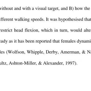
We useDelaunay triangulation [17, 18, 19] of a set of points to obtain our triangulated graphs. In Figure 1 a triangulated V–formation is shown with
V = {1,2,3,4,5,6,7}, Eo = {21,31,32,42,43,53,54,64,65,75,76}, Fo = {312,432,534,654,756}. (5)
1
2
3
4
5
6
7
.Figure 1: A triangulated V–formation.
Fix the edge and face orientation of the triangulated graphGsuch that for all the facesaijk≥0, i.e. if for the face ijk ∈ Fo ⊂ F, aijk <0 then replace the triplet (vi, vj, vk) ∈ Fo by (vj, vi, vk) to change the sign of the determinant in (3). The followingedge and face deviation variables (also known as shape variable [11]) associated with the edges and faces of the triangulated graph G are defined, respectively, as
ηij = kqj−qik −dij, ∀ij ∈ Eo
δijk = qik⊗qij := (qk−qi)TS(qj−qi)−aijk, ∀ijk∈ Fo, (6) whereqrs:=qs−qr and the tensor product ⊗is defined by α⊗β :=αTSβ forα, β∈R2.
Let pi = ˙qi denote the velocity of each node vi ∈ V. Then, the edge and face deviation rate variables (also known as shape velocities [11]) associated with the set of edges and faces of the graphG are defined, respectively, as follows:
νij := ˙ηij =
(pj−pi)T ·(qj−qi)
kqj −qik
=nTij ·(pj −pi), ∀ij∈ Eo
ξijk:= ˙δijk = (pk−pi)TS(qj−qi) + (qk−qi)TS(pj−pi), ∀ijk∈ Fo,
where nij =qij/kqijk forqi 6=qj. Using the notation prs =ps−pr and α⊥ := Sα (thus α⊗β =
αT ·β⊥), we can simplify the expression for the shape velocities as
νij := nTij·pij, ∀ij ∈ Eo
ξijk := pik⊗qij+qik⊗pij =pTik·qij⊥−pTij·q⊥ik, ∀ijk∈ Fo.
(8)
3
Formulation of the Optimization Problem
In this paper, we are interested in constructing a meaningful integrated cost function and ter-minal cost (respectively, L(x, u) and G(x) in (9)) for the purpose of performing a mission in a coordinated fashion using multiple vehicles with underactuated dynamics and constrained controls. More precisely, here, the mission of interest is tracking in formation for a group of underactuated hovercraft-type mobile robots with dynamics given in (31) and bounded control (i.e. ui ∈ U,∀i∈ I whereU 30 is a compact set (i.e. U = [0umax]2 ⊂R2)). The overall optimization problem can be expressed as the following:
J(x0) = min ˙ xi=f(xi, ui), ui ∈ U Z T 0 L(x, u)dt+G(x(T)), x(0) =x0, i∈ I, (9)
where x = col(x1, . . . , xn) and G(x) is a control Lyapunov function (CLF) for the concatenated dynamics of all vehicles ˙x = F(x, u) (the ith element of F is f(xi, ui)). To construct L(x, u) and G(x), we need to add several cost functions that each have a specific role in achieving our coordinated tracking objective. In the following, we explain how we obtain the terms that constitute
L(x, u) and G(x). The optimal control resulting from (9) is implemented in a receding horizon fashion.
4
Formation/Tracking Cost Decomposition
We demonstrate that the integrated cost for the problem of tracking in formation is constructed by decomposition of the task to formation stabilization with collision avoidance plus tracking. 4.1 Formation Cost
Letσ(x) :R→Rbe a continuous and locally Lipschitz function satisfying the following properties: i)σ(0) = 0, ii) (x−y)(σ(x)−σ(y))>0,∀x6=y. Then, based on ii),xσ(x)>0 andφ(x) =R0xσ(s)ds
is a positive definite and convex function which we refer to as a cost function. As an example, consider
σ(x) = √ x
x2+ 1 →φ(x) =
p
x2+ 1−1 (10) We define the potential-based cost and the kinetic-based cost associated with the formation graphG = (V,E,D,F,A), respectively, as the following
VG(q) := Pij∈Eoφ1(ηij) + P
ijk∈Foφ2(δijk),
TG(q, p) := Pij∈Eoφ3(νij) +Pijk∈Foφ4(ξijk),
whereφi(x) =
Rx
0 σi(s)ds, i= 1,2,3,4 and theσi’s satisfy conditions i) and ii). For the special case where all the σi’s are equal to the identity function, φi(x) = x2/2 and both VG, TG are quadratic functions of the shape variables and velocities. Here, we useφ1(x) =φ2(x) =φ3(x) =φ4(x) =x2/2 (note that the choice of φ1(x) =φ2(x) =
√
x2+ 1−1 is possible as well).
In general, corresponding to each edge shape variableηij, there exists a cost functionφij(x). Let Φη,Φν,Φδ,Φξ denote the set of cost functions associated with the set of variables ηij, νij, δijk, ξijk, respectively. We refer to Φf = (Φη,Φν,Φδ,Φξ) as the set of formation costs corresponding to graph
G. The pair (G,Φf) is called a (formation)cost graph. We refer to the formation Hamiltonian [10] given by
HG(q, p) =TG(q, p) +VG(q) (12) as theformation cost induced by the cost graph (G,Φf).
Definition 1. (equilibrium state) We sayx∗ = col(q∗, p∗)∈R4n is an equilibrium state of the cost graph (G,Φf) if and only ifHG(q∗, p∗) = 0.
Definition 2. (orbit) Let (R, b)∈SO(2)×R2 and satisfy the kinematic equations
˙
b = v
˙
R = Rωˆ (13)
Define the elements of the vectors ¯q,p¯as
¯
qi = Rqi+b ¯
pi = Rpi+Rωqˆ i+v. (14) The orbit of a pointx= col(q, p) is defined as [x] :={x¯∈R4n: ¯x= col(¯q,p¯)}.
Proposition 1. The formation costHG is invariant along the orbit of any pointx=col(q, p)∈R4n.
Proof. The proof is by direct calculation (the propertyRS=SR is the key in this proof).
4.2 Collision Avoidance Cost
One of the main challenges in formation stabilization for multiple vehicles regardless of any tracking is collision avoidance between vehicles that get too close to each other. Let qi, qj be two vehicles that are not necessarily neighbors of each other in graphG. Imagine a circularprotection zone with radiusr0 around each vehicle. Define thesafety variable between any two arbitrary vehicles vi and
vj as
µij =kqj−qik −r0. (15) Apparently, two vehicles collide ifµij =−r0. The objective is to satisfyµij >−r0. Furthermore, if two vehicles are already apart byr0, orµij ≥0, there is no need to worry about collision avoidance. Since no vehicle can physically apply an infinite force to avoid another vehicle, it is not reasonable to use potential (or barrier) functions of the typeV(qi, qj) =−log(kqi−qjk) orV(qi, qj) = 1/kqi−qjk between two vehicles with µij < 0. A numerically feasible alternative to applying forces with singularities is to use a constant repelling force between two vehicles with µij <0 and applying no force whenµij ≥0, i.e. we could use the potential function V(qi, qj) =ψ(kµijk) where
ψ(x) :=−min{0, x}= −x+|x|
A smooth approximation of this function is given by
ψ(x) :
−x+√x2+2
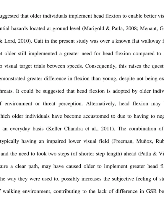
2 , 0< 1 (17) Both ψ(x), ψ(x) are depicted in Figure 2. Notice that
−10 −5 0 5 10 −2 0 2 4 6 8 10 12 ψ(x) ψε(x)
Figure 2: The functionψ(x) and its smooth approximationψ(x).
f(x) =−∇ψ(x) = 1 2(1− x √ x2+2) = 1 2(1−σ( x ))>0,∀x. (18)
This means that for x > 0 = 5, f(x)≈ 0. Now, define the following continuous approximation of f(x) ˜ f(x) := f(x)−f(0), x≤0 0, x > 0, (19) which satisfies the property ˜f(x)≥0,∀x. Define the positive semidefinite function
˜ ψ(x) :=− Z x 0 ˜ f(s)ds, (20) then, we have ˜ ψ(x) = 0,∀x≥0, ψ˜(x)>0,∀x < 0. (21) LetNi denote all the spatial neighbors of vehicle vi defined as follows:
Ni:={j ∈ I :kqj −qik ≤r0+0} (22)
By definition, we haveNi:={j ∈ I :µij ≤1}. Let us define the followingcollision avoidance cost
Vcol(q) = X i∈I X j∈Ni ψ(µij). (23)
If no two vehicles are spatial neighbor of each other, i.e. µij > 0,∀i < j ∈ I, then the collision avoidance cost is zero (Vcol(q) = 0).
Remark 1. The method that is presented here for construction of Vcol(q) is a distributed way of defining a collision avoidance cost for a multi-vehicle systemas compared to a centralized approach. In a centralized cost, there is a pair-wise potential functionψ(µij) between any two vehicle that will never vanish no matter how far the vehicles are from each other. The costVcol(q) can be calculated in a distributed manner because each vehicle needs to know about its local spatial neighborhood
Ni and not all other vehicles.
4.3 Tracking Cost
To perform the tracking, we choose a subgroup of vehicles called thecore vehicles to be in charge of doing the navigation and tracking in addition to trying to stay in formation withfollower vehicles, i.e. the vehicles that are not among the core vehicles. For doing so, we could choose a subgraph of the triangulated graphG = (V,E,D,F,A) called Gc which contains a subset of the faces inF with their corresponding edges and vertices. In its simplest form,Gc consists of a single triangle with the set of vertices Vc ={v1, v2, v3}. For simplicity of notation, we assume all vehiclesvi, i >3 are the followers. In general, the index set of the set of the core vehicles and the followers are denoted by
Jc and Jf, respectively. Notice that Jc∪Jf =I, Jc∩Jf =∅. Among the core vehicles, we choose one of the vehicles to be theattitude leader vj∗ [11], i.e. j∗ ∈Jc. Define the position and attitude
of the core formation as
qc = 1 |Jc| P j∈Jcqj, rc = qc−qj∗ kqc−qj∗k, (24)
where|Jc|denotes the number of members of the setJc. LetRc = [rc|rc⊥]∈SO(2), then ˙Rc =Rcωˆc defines ωc satisfying ˙θc = ωc. Here, θc is the angle of rc with the horizontal axis of the reference frame. Similarly, we can define the velocity of pc = ˙qc
pc = 1 |Jc| X j∈Jc pj (25)
This allows us to view the whole set of core vehicles as a single vehicle called theaggregated vehicle with the following dynamics:
aggregated vehicle: ˙ qc = pc, ˙ pc = uc, ˙ θc = ωc, ˙ ωc = τc, (26)
where xc = col(qc, pc, θc, ωc) ∈R6,uc ∈R2, andτc ∈R. Bothuc and τc can be directly calculated from the vehicles dynamics and the definition of qc, θc (it turns out that this calculation is not necessary to be done explicitly). Now, define a virtual vehicle called the navigator with the same dynamics as the aggregated vehicle:
navigator: ˙ qd = pd, ˙ pd = ud, ˙ θd = ωd, ˙ ωd = τd, (27)
with the initial conditions that are identical to the initial conditions of the aggregate vehicle. Let
yr(t) = col(qr(t), θr(t)) : R → R3 be a reference trajectory for the purpose of tracking. The navigator applies the following control input to achieve asymptotic output tracking ofyr:
ud = −c1(qd−qr)−c2(pd−q˙r) + ¨qr
τd = −c1(θd−θr)−c2(ωd−θ˙r) + ¨θr
(28) withc1, c2>0. With the idea of trying to force the aggregated vehicle to follow the navigator, we define the following tracking cost function:
Htr(xc, xd) :=φ5(qc−qd) +φ6(pc−pd) +φ7(θc−θd) +φ8(ωc−ωd), (29) wherexd= col(qc, pc, θc, ωc), φ5(x) =φ6(x) =kxk2/2, andφ7(x) =φ8(x) =x2/2. We take
L(x, xd, u) = L(x, xd) :=HG(q, p) +Htr(xc, xd) +Vcol(q)
G(x, xd) = HG(q, p) +Htr(xc, xd)
(30) The reason that the terminal cost G(x, xd) does not contain any collision avoidance cost is that it is assumed that in the final desired formation no vehicle is in the protection zone of any other vehicle, i.e. Ni =∅,∀i∈ I.
Definition 3. (tracking in formation) We say a group of vehicles achieve asymptotic tracking in formation if and only if the following conditions hold:
i) The formation of the vehicles asymptotically converges to the desired formation which is the equilibrium state of the cost graph (G,Φf).
ii) The outputyc = col(qc, θc) of the aggregated vehicle of the set of core vehicles asymptotically tracks the outputyr.
5
Underactuated Robot Dynamics
In this paper, we assume each vehicle is a hovercraft mobile robot with the following dynamics:
˙ qi = pi mp˙i = cos(θi) sin(θi) (u1i +u2i)−k1·pi ˙ θi = ωi I0ω˙i = r0(ui1−u2i)−k2·ωi (31)
where 0≤k1/m, k2/I0 1 and m, I0, r0 >0 are physical parameters of the vehicle dynamics. In addition, thecontrol inputs of each vehicle are positive and bounded or 0≤u1i, u2i,≤umax. In other words, the control ui = (u1i, u2i)T belongs to a compact set U as
ui ∈ U = [0umax]×[0umax] (32) For simplicity of notation, we represent the dynamics of each vehicle in (31) as the following
˙
with the state xi = col(qi, pi, θi, ωi)∈R6 and A= 02×2 I2×2 0 0 02×2 −k1/mI2×2 0 0 02×2 02×2 0 1 02×2 02×2 0 −k2/I0 , B(θi) = 0 0 0 0 cos(θi)/m cos(θi)/m sin(θi)/m sin(θi)/m 0 0 r0/I0 −r0/I0
Clearly, the system in (31) is an underactuated system with 3 degrees of freedom (DOF) and 2 control inputs.
6
Simulation Results
In this section we present the simulation results for tracking in formation for a group of six underac-tuated mobile robots with dynamics given in (31). The graph for the desired formation is shown in Figure 3 (each edge is of length 1). In the simulations that follow, the horizon time is 6 seconds and
3 2 1 4 5 6 . . .
Figure 3: A triangulated six–vehicle formation.
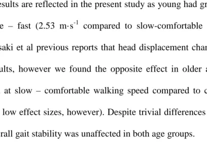
the update time is 1 second. Figure 4 (a) shows a 6-vehicle formation tracking a reference moving with constant velocity and heading. The vehicles are multi-colored and the reference vehicle is clear (white). The trajectories of each vehicle are denoted by lines with “x” marks for each receding horizon update.
The vehicles are initially lined up with a velocity of 1 in the horizontal direction, equal to the reference velocity. Note that without the collision avoidance cost term, vehicles 4 and 3 collide around 2.5 seconds. Figure 4 (b) shows snapshots of the evolution of the formation for the first 5 seconds of tracking.
Figures 5 (a) and (b) show the control inputs for vehicles 1 through 3 and vehicles 4 through 6, respectively. It can be observed that vehicle 6 in particular performs a rather aggressive maneuver, as the control goes to the constraint bounds for nearly 1 second. After 10 seconds, all vehicles reach a steady-state behavior.
The desired distance between any two neighboring vehicles the formation is 1. Figure 6 shows that vehicles 3 and 4 get close to each other without having a collision and eventually converge to the desired distance√3≈1.73 from each other.
7
Distributed Optimization: Remarks
The cost specification procedure detailed in the previous sections is beneficial not only because it is scalable to an arbitrary number of vehicles, but it also lends itself to a distributed implementation. We briefly describe such an implementation here, leaving the technical details for a future work.
The formation cost is additive, and consequently separable, with respect to the (edge and face) deviation and deviation rate variables. Note that even a single deviation variable is non-separable with respect to the positions of the end points of an edge. Assuming an agent is locally solving an optimization for the purpose of computing its own control, each such local optimization must account for the state of the neighbors of that agent on the graph. The tracking cost is induced by a subgraph of the full triangulated graph. Although the local optimization corresponding to the set of core vehicles must include a tracking cost, no new neighbors are introduced. The collision avoidance cost does introduce the requirement that any local optimization be able to account for the spatial neighbors of the corresponding agent, but this is a local requirement and the cost can be calculated in a distributed manner.
A challenging issue for a distributed implementation is to appropriately account for the graph/spatial neighbors in each local optimization. Of course, such an account must respect the appropriate timing modes (synchronous/asynchronous) and communication limitations. Currently, we are ex-ploring algorithms for distributing optimization problems with non-separable costs under various timing and communication assumptions.
8
Conclusion
In this paper, we introduced a graph theoretic framework for algebraic specification of a formation in an unambiguous way based on the notion of formation graphs. This specification allowed us to construct cost functions for formation stabilization, collision avoidance, and tracking which constitute three terms of the integrated cost and terminal cost of a finite horizon optimization problem. We presented tracking simulation results for a formation of six underactuated mobile robots. The obtained optimization problem is solved using the NTG software package. We also discussed the issues regarding the distribution of the main optimization problem in this paper
References
[1] C. W. Reynolds, “Flocks, herds, and schools: a distributed behavioral model,” Computer Graphics (ACM SIGGRAPH ’87 Conference Proceedings), vol. 21, no. 4, pp. 25–34, July 1987.
[2] C. W. Reynolds, “Interaction with a group of autonomous charachters,” in Proc. of Game Developers Conference. pp. 449–460, CMP Game Media Group, San Francisco, CA, 2000. [3] N. E. Leonard and E. Fiorelli, “Virtual leaders, artificial potentials, and coordinated control
of groups,” Proc. of the 40th IEEE Conference on Decision and Control, Orlando, FL, Dec. 2001.
[4] P. ¨Orgen, E. Fiorelli, and N. E. Leonard, “Formations with a mission: stable coordination of vehicle group maneuvers,” Proc. of the Symposium on Mathematical Theory of Networks and Systems, August 2002.
[5] J. P. Desai, J. P. Ostrowski, and V. Kumar, “Modeling and control of formations of nonholo-nomic mobile robots,” IEEE Trans. on Robotics and Automation, vol. 17, no. 6, December 2002.
[6] T. Eren, P. N. Belhumeur, B. D. O. Anderson, and S. A. Morse, “A framework for maintaing formations based on rigidity,” Proceedings of the 2002 IFAC World Congress, July 2002. [7] M. Mesbahi and F. Y. Hadegh, “Formation flying of multiple spacecraft via graphs, matrix
inequalities, and switching,” AIAA Journal of Guidance, Control, and Dynamics, vol. 24, no. 2, pp. 369–377, March 2000.
[8] R. W. Lawton, J. R. T. Beard and B. J. Young, “A Decentralized Approach to Formation Maneuvers,” IEEE Trans. on Robotics and Automation (to appear), 2002.
[9] M. Milam, K. Mushambi, and R. M. Murray, “A new computational approach to real-time trajectory generation for constrained mechanical systems,” Proc. of the 39th IEEE Conf. on Decision and Control, vol. 1, pp. 845–551, 2000.
[10] R. Olfati-Saber and R. M. Murray, “Distibuted cooperative control of multiple vehicle for-mations using structural potential functions,” The 15th IFAC World Congress, June 2002,
http://www.cds.caltech.edu/~olfati/papers/ ifac02/ifac02_ros_rmm.html.
[11] R. Olfati-Saber and R. M. Murray, “Graph Rigidity and Distributed Formation Stabilization of Multi-Vehicle Systems,” Proceedings of the IEEE Int. Conference on Decision and Control, Dec. 2002,http://www.cds.caltech.edu/~olfati/papers/ cdc02/cdc02a.html.
[12] G. Laman, “On graphs and rigidity of plane skeletal structures,” Journal of Engineering Mathematics, vol. 4, no. 4, pp. 331–340, October 1970.
[13] L. Lov´asz and Y. Yemini, “On generic rigidity in the plane,” SIAM J. Alg. Disc. Meth., vol. 3, no. 1, pp. 91–98, March 1982.
[14] J. Graver and H. Servatius, B. Servatius, Combinatorial Rigidity, vol. 2 of Graduate Studies in Mathematics, American Mathematical Society, 1993.
[15] M. Laurent, “Cuts, matrix completions, and graph rigidity,” Mathematical Programming, pp. 255–283, 1997.
[16] W. B. Dunbar and R. M. Murray, “Model Predictive Control of Coordinated Multi-Vehicle Formations,” Proceedings of the IEEE Conference on Decision and Control, Las Vegas, NV, December, 2002.
[17] L. Gubias and J. Stolfi, “Primitives for the manipulation of general subdivisions and the computation of voroni diagrams,” ACM Trans. on Graphics, vol. 4, no. 2, pp. 74–123, April 1985.
[18] R. A. Dwyer, “A Faster Divide–and–Conquer Algorithm for Constructing Delaunay Triangu-lations,” Algorithmica, vol. 2, no. 2, pp. 137–151, 1987.
[19] J. R. Shewchuk, “Triangle: Engineering a 2D Quality Mesh Generator and Delaunay Trian-gulator,” Proc. of the First Workshop on Applied Computational Geometry , pp. 124–133, Philadelphia, PA, 1996.
−4
−2
0
2
4
6
8
10
12
−1
0
1
2
3
x (m)
y (m)
Formation History
1 2 4 5 3 6 2 1 3 4 6 5 (a)−4
−2
0
−1
0
1
2
3
x (m)
y (m)
time = 0
−2
0
2
−1
0
1
2
3
x (m)
y (m)
time = 1
−2
0
2
−1
0
1
2
3
x (m)
y (m)
time = 2
0
5
−1
0
1
2
3
x (m)
y (m)
time = 3
2
4
6
−1
0
1
2
3
x (m)
y (m)
time = 4
4
6
−1
0
1
2
3
time = 5
x (m)
y (m)
(b)Figure 4: Trajectories of a six-vehicle formation: (a) the evolution and the path of the formation, (b) snapshots of the evolution of the formation (note: the two cones at the sides of each vehicle show the magnitudes of the control inputs).
0 2 4 6 8 10 0 2 4 6 Input Histories u11 u12 0 2 4 6 8 10 0 2 4 6 u21 u22 0 2 4 6 8 10 0 2 4 6 time u31 u32 (a) 0 2 4 6 8 10 0 2 4 6 Input Histories u41 u42 0 2 4 6 8 10 0 2 4 6 u51 u52 0 2 4 6 8 10 0 2 4 6 time u61 u62 (b)
Figure 5: Control inputs applied by each vehicle for the purpose of tracking in formation: (a) controls of vehicles 1 through 3, (b) controls of vehicles 4 through 6.
0 2 4 6 8 10 0 0.2 0.4 0.6 0.8 1 1.2 1.4 1.6 1.8 2 Distance ||q 3 − q4|| time