Essays on Development Economics

UC San Diego

UC San Diego Electronic Theses and Dissertations

Title

Essays on Development Economics Permalink

https://escholarship.org/uc/item/5dv129c8 Author

Vera Cossio, Diego Publication Date 2018

UNIVERSITY OF CALIFORNIA SAN DIEGO

Essays on Development Economics

A dissertation submitted in partial satisfaction of the requirements for the degree of Doctor of Philosophy

in

Economics

by

Diego Alejandro Vera Cossio

Committee in charge:

Professor Prashant Bharadwaj, Chair Professor Gordon Dahl

Professor Craig McIntosh Professor Karthik Muralidharan Professor Krislert Samphantharak

Copyright

Diego Alejandro Vera Cossio, 2018 All rights reserved.

The Dissertation of Diego Alejandro Vera Cossio is approved and is acceptable in quality and form for publication on microfilm and electronically:

Chair

University of California San Diego 2018

DEDICATION

To my beloved mom, Maria Elena, for her constant motivation and encouragement to pursue my dreams. She may no longer be with us, but I am sure she is enjoying this accomplishment from Heaven. To my brother, Horacio, for always filling in for me during this long time away from home. To my dad, Walter, for dedicating his life to provide us with opportunities. To my aunt, Maria Luisa, for providing her loving support. To Ashley, for being my unconditional partner in this journey.

EPIGRAPH

Poverty is not just a lack of money; it is not having the capability to realize one’s full potential as a human being.

TABLE OF CONTENTS

Signature Page . . . iii

Dedication . . . iv Epigraph . . . v Table of Contents . . . vi List of Figures . . . ix List of Tables . . . xi Acknowledgements . . . xiv Vita . . . xv

Abstract of the Dissertation . . . xvi

Chapter 1 Targeting Credit . . . 1

1.1 Introduction . . . 2

1.2 The village financial system and the Village Fund program . . . 9

1.2.1 The village financial system . . . 9

1.2.2 The Million Baht Village Fund program . . . 10

1.2.3 Local elites and the MBVF program . . . 11

1.3 The Village Fund committee as a social planner . . . 12

1.4 Data and measurement . . . 17

1.4.1 Measuring poverty . . . 18

1.4.2 Measuring pre-program productivity . . . 18

1.4.3 Measuring repayment behavior . . . 23

1.4.4 Measuring connections with local elites . . . 24

1.5 Targeting analysis . . . 25

1.5.1 Comparisons of program beneficiaries and non-beneficiaries . . . 25

1.5.2 Poverty targeting , productive efficiency and repayment . . . 26

1.5.3 Discussion . . . 28

1.6 Access to credit from the program, connections with local elites, and favoritism 29 1.6.1 Favoritism towards connected households . . . 31

1.6.2 Discussion . . . 34

1.7 Program spillovers to unconnected households . . . 35

1.7.1 Empirical strategy . . . 35

1.7.2 Results . . . 37

1.7.3 Threats to identification, robustness, and attrition . . . 39

1.8 Concluding remarks and discussion . . . 40

1.10 Tables . . . 49

1.11 Acknowledgements . . . 56

Chapter 2 Cash Transfers and Labor Supply . . . 57

2.1 Introduction . . . 58

2.2 The setting . . . 63

2.3 Data . . . 65

2.4 Identification strategy . . . 66

2.5 Labor supply responses and the CCT program . . . 68

2.5.1 Cash or condition? . . . 70

2.6 Dependence or constraints? . . . 73

2.6.1 Testing the implications of the model . . . 79

2.7 Potential alternative mechanisms . . . 82

2.8 Robustness checks and methodological issues . . . 83

2.9 Concluding remarks and discussion . . . 84

2.10 Figures . . . 87

2.11 Tables . . . 96

2.12 Acknowledgements . . . 102

Chapter 3 Access to Credit and Productivity . . . 103

3.1 Introduction . . . 104

3.2 Context and Data . . . 109

3.3 A simple theoretical framework . . . 110

3.4 Empirical strategy . . . 112

3.4.1 Production function estimation . . . 115

3.5 Reduced-form results . . . 120

3.5.1 Effects on program and total short-term credit . . . 120

3.5.2 Effects on household income . . . 121

3.5.3 Effects for owners of pre-existing businesses . . . 122

3.5.4 Robustness . . . 124

3.6 IV estimates of the returns to credit . . . 125

3.6.1 Implied rates of return to investments on business assets . . . 126

3.7 Concluding remarks and policy implications . . . 127

3.8 Figures . . . 130

3.9 Tables . . . 134

3.10 Acknowledgements . . . 142

Appendix A Appendix for Chapter 1 . . . 143

A.1 Supplementary figures and tables . . . 143

A.2 Productivity . . . 161

A.2.1 Identification assumptions . . . 162

A.3 Robustness to the agricultural cycle and placebo analysis . . . 177

A.3.1 Attrition . . . 180

Appendix B Appendix for Chapter 2 . . . 188 B.1 Supplementary figures and tables . . . 188

B.1.1 Effects Excluding Children with Siblings with Different Treatment Status 192

B.1.2 Heterogeneous Treatment Effects by Counterfactual Attendance Rate . . 194

Appendix C Appendix for Chapter 3 . . . 199 C.1 Supplementary figures and tables . . . 199 Bibliography . . . 208

LIST OF FIGURES

Figure 1.1. Access to Credit, Poverty and Productivity . . . 44

Figure 1.2. Access to Credit and Connections with the Elites . . . 45

Figure 1.3. Short-term Effects of on Credit From Informal Lenders . . . 46

Figure 1.4. Short-term Effects on Credit From Relatives for Unconnected Households 47 Figure 1.5. Short-term Effects on Non-program Institutional Credit (BAAC) . . . 48

Figure 2.1. Gender Gap in Employment . . . 87

Figure 2.2. Cash Reception . . . 88

Figure 2.3. Work Hours: Adults . . . 89

Figure 2.4. Number of Adults Working . . . 90

Figure 2.5. Employment and Hours Worked (weekly) for Adults . . . 91

Figure 2.6. Effects on Total Labor Supply . . . 92

Figure 2.7. Treatment Effects on Employment and Hours for Adults . . . 93

Figure 2.8. CDF of Predicted Attendance Rate . . . 94

Figure 2.9. Effects on the Extensive Margin of Work . . . 95

Figure 3.1. Effects of the program rollout on short-term credit . . . 130

Figure 3.2. Reduced-form effects on household income - Proxy-variable approach . . . 131

Figure 3.3. Reduced-form effects on business profits - Business owners only . . . 132

Figure 3.4. Effects on business assets . . . 133

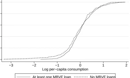
Figure A.1. Cumulative Distribution Functions of Baseline Consumption and Produc-tivity by Different Criteria . . . 144

Figure A.2. Average Village Lending . . . 147

Figure A.3. Short-term Effects on Lending to Other Households . . . 150

Figure A.5. Loan Portfolio Before and After the Program . . . 160

Figure A.6. Productivity and Intermediate Inputs . . . 175

Figure A.7. Short-term on Credit from Local Informal Sources . . . 178

Figure A.8. Short-term Effects on Credit from Relatives- Unconnected Households . . . 179

Figure B.1. Effects on Total Household Labor Supply . . . 190

Figure B.2. Effects on Employment for Adults (1st-8th grade) . . . 191

Figure B.3. Employment and Work Hours (weekly) for Adults . . . 192

Figure B.4. Predicted and Observed Attendance Rates . . . 194

Figure C.1. Effects of program rollout on household income - Fixed-effects approach . 202 Figure C.2. Effects of program rollout on household income . . . 204

LIST OF TABLES

Table 1.1. Program Participation, Poverty and Productivity . . . 49

Table 1.2. Difference with Means-Testing Criterion . . . 50

Table 1.3. Differences with Credit-Scoring Criterion . . . 51

Table 1.4. Access to Credit, Connections, and Borrower Characteristics . . . 52

Table 1.5. Differences in Loan Outcomes by Connections with the Elites . . . 53

Table 1.6. Short-run Program Effects on Credit from Informal Lenders . . . 55

Table 2.1. Program Design . . . 67

Table 2.2. Summary Baseline Statistics . . . 96

Table 2.3. Testing for Parallel Trends . . . 97

Table 2.4. Effects on Employment . . . 98

Table 2.5. Effects on Self-employment: Adult Females . . . 99

Table 2.6. Adult Females: Heterogeneous Treatment Effects by Counterfactual Atten-dance Rate . . . 100

Table 2.7. Adult Females: Heterogeneous Treatment Effects by Access to Credit . . . . 101

Table 3.1. Baseline Summary Statistics . . . 134

Table 3.2. Estimates of Value-added Production Functions . . . 135

Table 3.3. Reduced-form Effects of the Program on Household Profits . . . 136

Table 3.4. Reduced-form Effects of the Program on Off-farm Business Activities . . . . 138

Table 3.5. IV Estimates of the Effects of Total Credit on Income and Profits . . . 139

Table 3.6. IV Estimates of the Effect of Total Credit on Off-farm Businesses (Pre-existing Businesses Only) . . . 140

Table A.1. Distribution of Targeted Households by Alternative Criteria . . . 143

Table A.2. Connections and Baseline Borrower Characteristics . . . 145

Table A.4. Effects on Program and Total Borrowing . . . 148

Table A.5. Short-run Effects on Credit from Non-program Institutional Lenders . . . 149

Table A.6. Short-run Effects on Lending to Other Households . . . 151

Table A.7. Summary Statistics for Baseline Characteristics( 1999-2000) . . . 153

Table A.8. Summary Statistics for Credit Adoption by Type of Lender . . . 154

Table A.9. Demographic Characteristics by Membership in the Village Council . . . 155

Table A.10. Baseline Socioeconomic and Kinship Relationships with Village Council Members . . . 157

Table A.11. Summary Statistics for Connections with the Elite . . . 158

Table A.12. Poverty and Productivity by Baseline Access to Credit and Alternative Targeting Criteria . . . 159

Table A.13. Value Added Function Estimates . . . 170

Table A.14. Production Function Estimates Under Alternative Specifications . . . 173

Table A.15. Test for Frictions in Intermediate Inputs . . . 176

Table A.16. Effects on Total Borrowing (Excluding Attriters) . . . 180

Table A.17. Effects on Informal Credit (Excluding Attriters) . . . 181

Table A.18. Effects on Total Borrowing by Connectedness Score . . . 182

Table A.19. Effects on Informal Credit by Connectedness Score . . . 183

Table B.1. Treatment Effects: Parents of Children from 1st to 8th Grade . . . 189

Table B.2. Effects Excluding Children with Siblings with Different Treatment Status . 193 Table B.3. Heterogeneous Treatment Effects by Counterfactual Attendance Rate . . . 195

Table B.4. Treatment Effects on Enrollment and Employment (Children) . . . 196

Table B.5. Adult females: Heterogeneous Treatment Effects by Access to Credit . . . 197

Table B.6. Effects on Self Employment-Adult Females . . . 198

Table C.2. Correlation between Within-village Productivity Rankings . . . 200

Table C.3. Correlates of baseline productivity and demographic characteristics . . . 201

Table C.4. Reduced-form effects of the program on off-farm business activities-

Win-sorized . . . 203

Table C.5. IV Estimates of the Effects of Program Credit on Income and Profits . . . 206

ACKNOWLEDGEMENTS

I would like to thank Professor Prashant Bharadwaj for his support as the chair of my committee. His commitment to my work and his encouragement were fundamental. I feel lucky for having had him as an advisor. I am also very grateful to Gordon Dahl, Craig McIntosh, Karthik Muralidharan and Krislert Samphantharak for always willing to spend time discussing my research.

I would like to thank my peers, Desmond Ang and Mauricio Romero, for valuable feedback and providing great company during the job-market process. Similarly, I would like to acknowledge Patrick Bloom, Dodge Cahan, Mitch Downey, Kilian Heilman, Claudio Labanca, Bruno Lopez, Julian Martinez, Pablo Ruiz and Gonzalo Valdez for making my experience at UCSD a pleasant one.

I would also like to acknowledge my co-authors, Robert Townsend and Emily Breza. Chapter 1, is currently being prepared for submission for publication of the material. Vera Cossio, Diego ”Targeting credit through community members”.

Chapter 2, is currently being prepared for submission for publication of the material. Vera Cossio, Diego ”Dependence or constraints? Cash transfers and female labor supply”.

Chapter 3, is currently being prepared for submission for publication of the material. Breza, Emily; Townsend, Robert; Vera Cossio, Diego ”Access to credit and productivity: evidence from Thai Villages”. The dissertation author has contributed significantly to the collaborative research.

VITA

2008 Bachelor of Arts, Universidad Catolica Boliviana San Pablo. La Paz, Bolivia.

2009–2010 Research Assistant, Institute of Advanced Development Studies INESAD. La Paz,

Bolivia.

2011 Master of Arts in Economics. Universidad de Chile. Santiago, Chile.

2012-2013 Research Fellow, Inter-American Development Bank. Washington, District of

Columbia. USA

2018 Doctor of Philosophy in Economics. University of California, San Diego.

FIELDS OF STUDY Major Field: Development Economics

ABSTRACT OF THE DISSERTATION

Essays on Development Economics

by

Diego Alejandro Vera Cossio

Doctor of Philosophy in Economics

University of California San Diego, 2018

Professor Prashant Bharadwaj, Chair

A fundamental concern in development economics is the presence of institutional and labor market failures that interact with frictions in financial markets, which may prevent economic growth. This dissertation studies the importance of these interactions in a series of three papers. Chapter 1 studies the extent to which by allowing grassroots organizations–as opposed to banks–to allocate publicly-funded credit, it is possible to overcome existing financial frictions and deliver resources the community members who need it the most: poor, high-productivity households. Using a long panel dataset I find evidence of misallocation: credit was provided to households with poor credit history, which were richer and less productive than non-borrowers. Instead, resources were delivered to households with connections to local political leaders. The

results highlight the limitation of community-based approaches to allocating public resources in developing countries. Chapter 2 shows that a cash-transfer program targeted to children in Bolivian public schools boosted employment among mothers of beneficiary children by providing extra-liquidity in a context of fixed costs to work. Chapter 3 exploits rich data from Thailand to show that estimates of total factor productivity can be used to predict business success in the aftermath of credit-expansion programs.

Chapter 1

Targeting Credit through Community

Members

Abstract

Delegating the allocation of public resources to community members is an increasingly popular form of delivering public resources in developing countries. However, this approach is associated with the tradeoff between improved information about potential beneficiaries and favoritism towards local elites, which could be strengthened in the context of credit. Unlike targeting cash transfers to the poor, the optimal targeting of credit is a more complex problem involving issues of productivity, repayment, and market responses: This paper analyzes this problem using a large-scale lending program, the Thai Million Baht Credit Fund, which decen-tralizes the allocation of loans to an elected group of community members, and provides three main results. First, exploiting a long and detailed panel, I recover pre-program structural esti-mates of household productivity and find that resources from the program were not allocated to high-productivity, poor households, which is inconsistent with poverty and productive efficiency as targeting criteria. Second, using socioeconomic networks data, I show that actual targeting is strongly driven by connections to village elites and is related to lower program profitability, which suggests favoritism as a reason for mistargeting. Finally, I exploit quasi-experimental variation in the rollout of the program and uncover evidence that, in general equilibrium, informal credit markets compensate for targeting distortions by redirecting credit towards unconnected

households, albeit at higher interest rates than those provided by the program. The results highlight the limitations of community-driven approaches to program delivery and the role of markets in attenuating potential targeting errors.

1.1

Introduction

Community-driven development approaches to delivering public resources have gained increasing attention from academics and policy makers around the world. In developing countries, a number of social programs such as public works or cash transfer programs rely on community

members for their implementation or monitoring.1 One of the foundations of this approach is the

idea that community members, as opposed to traditional policy makers, have better information to identify local needs. In the context of credit, delegating the allocation of resources to community members may lead to more accurate identification of potential borrowers and may fulfill the promise that was only partially materialized by traditional microfinance: providing affordable

credit to poor, high-productivity households.2

One important class of community-based policies to expand access to credit is that of government infusions of resources into villages for the establishment of local credit funds which

are managed by elected groups of community members.3 The economic rationales for this

approach include the reduction of intermediation and administrative costs as well as the benefit

1_{See for example Mansuri and Rao (2004) for a review in the case of community-based approaches to}

infrastruc-ture projects. Community based targeting of cash transfers has been studied by Alatas et al. (2012), and participatory rankings among community members have been used in graduation programs (Banerjee et al., 2015), and other programs that involved the delivery of cash transfers to the ultra poor (Bandiera et al., 2017).

2_{Uptake of credit in recent microcredit interventions has been low, due to, among other reasons, high interest}

rates and the difficulty of identifying high-productivity borrowers (Banerjee et al., 2015; Crpon et al., 2015; Banerjee et al., 2015). Reviews from either a policy or an academic perspective regarding the challenges of microfinance are provided by World Bank (2008); Armend´ariz de Aghion and Murdoch (2004); Banerjee and Duflo (2010); Morduch (1999); Karlan and Morduch (2010).

3_{Broadly, community-based credit approaches consist of fostering local credit funds to be managed by community}

members. A clear example is the Million Baht program in Thailand (Kaboski and Townsend, 2012) and the Integrated Rural Development Program in India (Bardhan and Mookherjee, 2006b). While self-funded village credit groups are a growing research topic in the literature (see Deininger (2013); Greaney et al. (2016); Ksoll et al. (2016); Karlan et al. (2017), among others), there are other types of government-funded programs with a community based approach around the world such as the Andhra Pradesh Rural Poverty Reduction Project in India, and the Rural Financial Institutions Programme in Uttar Pradesh.

from information available to community members, which is costly to obtain by policy makers. On the other hand, community members may engage in favoritism towards politically connected households (Bardhan and Mookherjee, 2005). This tension is particularly salient in cases in which community members disperse public funds based on criteria that are hard to observe (unlike poverty targeting) and subject to moral hazard, as is the case with credit markets. Thus, whether the allocation of resources is consistent with poverty, productive efficiency or favoritism as targeting criteria is an empirical question. While the ability of community members to identify profitable households has been documented (Hussam et al., 2017), little is known regarding the effective use of this information when community members themselves are in charge of the allocation of public credit. Moreover, although the use of pre-program data has been essential for the empirical analysis of community-based approaches to delivering resources to the needy (Alatas et al., 2012), other studies analyzing how local leaders allocate productive resources are based on post-program measures of productivity which are likely to be affected by the program itself (Bardhan and Mookherjee, 2006b; Basurto et al., 2017). In addition, previous studies have focused only on understanding how community members allocate resources but have ignored the role of markets in reallocating resources, which may attenuate potential targeting errors.

This paper empirically assesses these issues in the context of the Thai Million Baht Village Fund (MBVF) which is one of the largest community-based credit programs. Between 2001 and 2002, the government donated resources to over 90% of rural villages for the creation of local credit funds, which represented, on average, a 25% increase in the available funds for credit in each village. These funds were fully managed by elected village committees made up

of community members, who decided who obtained credit and under what loan conditions.4

This paper reports results from three empirical exercises: first, using a long panel, I structurally

4_{The importance of this program and the fundamental tradeoffs in the allocation of productive resources have}

been of interest in the literature, but there are both unanswered questions and methodological limitations to existing studies. Kaboski and Townsend (2012) and Kaboski and Townsend (2011) have documented the effects of the MBVF on several household outcomes and the cost-effectiveness of the program. Breza et al. (2017) analyze whether baseline productivity explains heterogeneity in the effects of the program on investment and income growth but do not explore the mechanisms behind the allocation of resources from the program. Thus, what the program’s

estimate a household production function and use the estimated factor elasticities to recover

pre-programestimates of household total factor productivity.5 I combine these estimates with

baseline per-capita consumption data to test:(i)whether village committee members delivered

credit to poor, high-productivity households, and(ii)whether offering credit to villagers based

on alternative targeting criteria (i.e., means-testing and a baseline repayment probabilities) would have delivered credit to poor, high-productivity households. Second, I combine detailed data on pre-program socioeconomic networks with data about loan characteristics and repayment to test for favoritism towards households with connections to the local elite. Third, I use quasi-experimental variation in the rollout of the program to test for within-village general equilibrium responses in credit markets, which could lead to program spillovers to households with limited access to credit from the program.

First, I find that the program does not target poor, high-productivity households and that, in terms of poverty and productive efficiency, the program is outperformed by alternative targeting criteria. In practice, the allocation of loans was regressive and productively inefficient: the distribution of baseline per-capita consumption corresponding to program beneficiaries first-order stochastically dominated that of non-beneficiaries. Moreover, only 40% of high-productivity households (top 25% of the high-productivity distribution) borrowed from the program, and , on average, program borrowers had lower baseline productivity than non-borrowers. This allocation was not consistent neither with concerns regarding equity nor repayment. By comparing program borrowers to households that would have been eligible under an alternative targeting criterion based on baseline wealth rankings (i.e., means testing), I find that, on average, the means-testing criterion would have targeted the poorest households without sacrificing productivity. Furthermore, by comparing program borrowers to households that would have been eligible under an alternative targeting criterion based on baseline repayment probabilities (i.e., repayment score), I find that 38% of households who received credit from the program would

5_{Concretely, I exploit data on households’ financial statements, in particular balance sheets, to measure capital}

as the value of the stock of total fixed assets for each household. The financial accounts data was compiled by Samphantharak and Townsend (2010).

have been ineligible under the repayment-score criterion. On average, these households were 12% less productive than households who did not borrowed from the program but exhibited high repayment probabilities. Reallocating program resources across these groups would have led to an average productivity gain of 4.5%, at no cost in terms of baseline per-capita consumption.

Second, while neither poverty targeting nor productive efficiency were the relevant allocation criteria, subsidized credit was disproportionately allocated to households with socioe-conomic connections to the local elite. Combining socioesocioe-conomic networks data and data on baseline membership in the village council (the highest political authority in each village), I

classify households as connected with the elite if theyi) are members of the village council,

ii)are first-order kin of the local elite, oriii)had direct pre-program socioeconomic ties to the

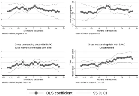
local elite. I find that connected households are 20 percentage points more likely to obtain credit from the program than unconnected households. Connected households were not poorer or more productive than unconnected households, and yet they obtained more credit. Moreover, connected households already had access to institutional credit before the program and had similar baseline delinquency rates. While the correlation between program participation and connection to local elites falls by 45% after controlling for total number of connections in the village, demographic characteristics, business orientation, and credit history, connected house-holds were still 10 percentage points more likely to obtain credit from the program. Thus, the slanted allocation towards connected households was only partially explained by improvements in information regarding borrower characteristics.

I find evidence of favoritism towards connected households with implications for program

profitability. Connected households were favored with low initial interest rates leading toex post

lower internal rates of return for the program. A cross-section sample of loans corresponding to 344 households who borrowed both from the program and privately funded local credit groups allows me to compare loan performance across different lenders for the same household and

control for unobserved borrower characteristics.6 I test for favoritism by analyzing whether

connected households obtain more favorable loan conditions in the case of program loans compared to loans from private credit groups and comparing these differences to those for unconnected households. The results show that program loans to connected households were granted at lower initial interest rates (1.5 percentage points). These differences compromised the

profitability of the program: theex postinternal rate of return on program loans to connected

households is 2 percentage points lower than the return on privately funded loans (on average 7%). These results are driven by differences for connected households, as there were no detectable differences for unconnected households.

Third, while committee members favored connected households and the program might not have directly reached unconnected households, the program indirectly benefited unconnected households by increasing the supply of overall credit available in the village. Aggregate borrow-ing increased by 24% in the sample villages within a year from the rollout of the program. Usborrow-ing high-frequency data, I exploit cross-village variation in the monthly rollout of the program to identify the short-term effects of the program on credit use for unconnected households. While connected households benefited directly from the program, unconnected households obtained loans from other lenders in the system. Event-study estimates for unconnected households show that borrowing from informal lenders increased by 30%; this result was mostly driven by loans from relatives. I also find suggestive evidence of an increase in formal borrowing for unconnected households, albeit at higher interest rates than those from the program. There was also re-lending: the probability of lending to other households increased by 2 percentage points in the case of connected households. Overall, spillovers mildly offset the difference in program borrowing between connected and unconnected households: back of the envelop calculations suggest that these effects only account for one-third of program-borrowing gap between connected and unconnected households.

This paper makes three main contributions to the literature studying community-based approaches to distributing public resources. First, it highlights the limitations of these approaches

to distribute productive resources when attributes of program beneficiaries are not easily observ-able by most community members. Unlike the context of poverty targeting, in the context of credit, the relevant targeting criteria may only be observable by direct economic interactions, strengthening the tension between information and favoritism. Alatas et al. (2012) provide evidence that households with connections to local elites are not more likely to receive cash transfers when resources are allocated by community members relative to a proxy-means-testing targeting criterion. The results from this paper show that this pattern may not hold in the case of credit and are consistent with evidence of favoritism in financial markets in the context of banks and firms (Khwaja and Mian, 2005; Haselmann et al., 2017). In addition, while Hussam et al. (2017) show that community members can identify productive households in India, this paper shows that accurate use of information may depend on social connections. In practice, both lack of information about unconnected households and favoritism can impose higher program-participation costs to households without the relevant connections, with consequences for poverty targeting, productive efficiency, and program sustainability. These losses should be considered whenever policy makers choose among alternative approaches to program delivery.

The second contribution to the targeting literature is methodological. The use of pre-program data has been central to the assessment of community-based approaches to allocate cash transfers to the needy (Alatas et al., 2012). However, studies evaluating the productive efficiency of community-based allocations rely on contemporary or post-program measures of productivity (Bardhan and Mookherjee, 2006b; Basurto et al., 2017). This paper improves previous empirical

assessments by exploiting a long panel dataset to recoverpre-programstructural estimates of

household productivity, which are unlikely to be affected by the program. In terms of results, using self-reported data collected after the implementation of a fertilizer subsidy program in Malawi, Basurto et al. (2017) provide evidence of a tradeoff between targeting the poor and targeting high-return households. Using post-program structural estimates of baseline household productivity, I show that such a tradeoff was not relevant in the more general case of credit.

implemen-tation of a large-scale program, this paper examines the targeting problem both from a partial and general equilibrium perspective. The literature has generally focused only on the targeting or screening process. This paper expands the analysis beyond the program and tests the

conse-quences of thede factotargeting criterion on village credit markets. By providing novel evidence

on the role of informal credit markets in attenuating targeting errors, this paper contributes to the literature documenting general equilibrium effects and spillovers from large-scale programs (Angelucci and De Giorgi, 2009; Muralidharan et al., 2017; Kaboski and Townsend, 2012). In particular, the results show that economic connections and political economy factors can affect not only the distribution of public resources in the village economy, but also the redistribution of these resources through markets (Kinnan and Townsend, 2012; Acemoglu, 2010). More broadly, the results suggest that a complete understanding of targeting problems should involve an analysis of how resources are redistributed across agents.

The results from this paper also build on the literature studying the introduction of micro-credit products in developing countries. A core concern in the development economics literature is that of delivering affordable credit to poor, high-productivity households to enable them to escape poverty traps (Banerjee and Duflo, 2010; Morduch, 1999). While the literature has mostly focused on studying the effects of the introduction of credit products on several

household outcomes,7 an empirical assessment of the productive efficiency of the allocation

of credit in large-scale programs has not yet been provided. My results show that even with low intermediation and administrative costs, credit from the MBVF program did not reach poor, productive households. A comparison of these results with those from studies analyzing selection into credit highlights the importance of different screening mechanisms in credit markets. For instance, Beaman et al. (2014) show that high-return households select into credit in a context

7_{Banerjee et al. (2015) provide a review of six randomized controlled trials studying the introduction of}

microcredit products in a varied of contexts. In particular, Banerjee et al. (2015) and Crpon et al. (2015) document low uptake rates in contexts in which credit was not directly offered to entrepreneurs. Deininger (2013) analyzes the impacts of access to credit on members of self-help groups. Kaboski and Townsend (2012) also provide an assessment in the context of the MBVF program.

in which the screening mechanism is price.8 This paper documents a less efficient result in a

context in which thede factoscreening mechanisms are social connections with local elites.

1.2

The village financial system and the Village Fund

pro-gram

1.2.1

The village financial system

The context of this study corresponds to Thai villages, an environment in which most households own land (80%) and obtain over one-third of their revenues from agricultural activi-ties (see Appendix table A.7). While most households obtain revenues from cultivation activiactivi-ties, the average household obtains revenues from 4 different economic activities: most households also obtain revenues from wage labor (78%), fishing and shrimping (40%) and off-farm family businesses (30%). To finance their economic activities, households borrow either from insti-tutional lenders, informal lenders or relatives. Among instiinsti-tutional sources of credit there are formal lenders, mainly the state-owned Bank of Agriculture and Agricultural Cooperatives

(BAAC), and quasi-formal lenders such as savings and credit groups and cooperatives.9 In terms

of the quantity of loans, half come from informal sources, while formal and quasi-formal sources

of credit provide over 70% of the total loan amount in the village financial system.10 On average,

households hold more than one loan and around one-third of the households hold informal loans (see Appendix Table A.8), which have higher interest rates than formal or quasi-formal loans.

8_{They do so in the context of a micro-credit program in Mali, managed by an NGO with no government}

intervention at all.

9_{Quasi-formal institutions include organizations that have a set of procedures for recording their operations,}

but do not have a physical location. Examples of these are production credit groups (PCGs), women’s groups and other village credit groups. See Kaboski and Townsend (2005) for a detailed description of these quasi-formal organizations in the Thai context.

10_{The top panel in Figure A.5 illustrates the structure of the portfolio of loans associated with the villages in}

the study sample, both in terms of the number of loans and the amount of credit provided before the program was implemented.

1.2.2

The Million Baht Village Fund program

The Million Baht Village Fund (MBVF) program consisted of an initial transfer of THB 1 million (USD 22,500 in 1999 values), from the Government of Thailand to rural and peri-urban

villages.11 The aim of the program was to stimulate the village economies by expanding access

to credit; program funds were used as seed capital for the creation of revolving credit funds in

95% of all villages in Thailand.12 Moreover, the program increased the aggregate gross lending

portfolio by 24% during the first year of its implementation in the sample villages, and modified significantly the composition of the portfolio of loans in each village (See and Appendix Figure A.5). The program offered loans at an average interest rate of 7% per year, which was the lowest rate in the market at that time: The average interest rate for other institutional loans was 11% per year . The program represents an unexpected event in that it was announced following a change in government and rapidly reached borrowers: As of the second year of implementation, the program had provided individual liability loans to 62% of households in the study sample.

The MBVF program differs from formal lenders in its management, relying on community members to manage credit funds. While there are other local savings and credit groups in which community members manage funds, they differ from the MBVF program in the way that they are

funded: The MBVF is mostly subsidized, and local credit and saving groups are self-funded.13

In each village, the MBVF program is managed by a village fund committee (VFC),a group of 10-12 elected community members that is responsible for evaluating loan applications and

monitoring loans.14 Committee members generally met once or twice a year to review loan

applications. While the program was governed by a set of regulatory guidelines, committee

11_{Average loan size is approximately USD 450 which represents roughly 25% of a households’s yearly income.} 12_{A detailed discussion of the application process that villages were required to follow to get access to the funds}

and the way in which those funds were delivered is provided by Kaboski and Townsend (2012), Boonperm et al. (2013), Menkhoff and Rungruxsirivorn (2011) and Haughton et al. (2014).I do not address that process here as all of the villages in the sample participated in the program.

13_{In order to borrow, households were require to purchase a share of the fund, at a very low costs. However, the}

funds themselves come from a one-time transfer by the Government.

14_{The members of the Village Fund Committee were elected for a 2 year term in a transparent setting and received}

a small compensation for their services (Menkhoff and Rungruxsirivorn, 2011), however Haughton et al. (2014) documents that most of the members continued in the position for several years.

members had full discretion to approve or deny applications and set loan amounts, terms, and

the initial interest rate.15 Although the Central Government provided villages with incentives

for sustainable management and sanctions in case of mismanagement, there were no direct incentives for committee members.

1.2.3

Local elites and the MBVF program

Each Thai village is governed by a village head and a group of advisors who make up the village council; they are hereinafter referred to as the “local elite”. The Village Council members are elected by villagers, appointed by district authorities, and usually serve in office

until retirement.16 The Village Council represents the main link between community members

and higher-level authorities. For instance, village council members attend district meetings, collect resources from villagers for religious celebrations or public works, and oversee resolution of disputes between villagers (Moerman, 1969; Mabry, 1979). In the study sample, Village Council members are richer, have larger extensions of land, and are more likely to have off-farm family businesses (see Appendix Table A.9).

The village fund committee wasde jurean independent entity, but it is possible that the

local elite, had enoughde factoauthority to influence committee decisions. Although the election

of village fund committee members is intended to induce accountability in the allocation of loans, committee members may have incentives to favor their political supporters or households with connections to the local elite. For instance, when elections could not take place, the

committee members were appointed by the village Head.17 The local elites could indirectly

influence committee members through their economic or family connections: On average, 46% of households in the sample report transacting with village council members during the two years

15_{The most important of these regulations were that loans could not exceed THB 20,000, a positive interest rate}

had to be imposed on all loans, the initial loan term could not exceed one year, and collateral could not be required, although households had to have one or two cosigners.

16_{This was the case during the study period. However, a reform in 2011 established 5 year terms, but allowed}

Village Heads to run for reelection.

17_{Haughton et al. (2014) document that 15% of village fund committee members were appointed directly by}

preceding the program and 13% of sample households are direct relatives of elite members (see Appendix Table A.10). In addition, relatives of the local elite could end up in charge of the funds

even in transparent elections. 18 Moreover, households with business connections to local elites

could use their privileged position to influence loan allocation decisions or to obtain preferential treatment. In such a context, the potential gains in information from decentralizing the allocation of resources to community members could be undermined by rent-seeking behavior (Bardhan and Mookherjee, 2005).

1.3

The Village Fund committee as a social planner

The central aim of this paper is to evaluate the allocation of resources by community members. The program’s stated objective was to establish credit funds in order to expand access to institutional credit and promote career development and income generation (Government of Thailand, 2004), which suggest that poverty, productivity and repayment were important dimensions to be considered. For instance, access to institutional credit was particular low among

the poor19, the government claimed publicly that resources were allocated to productive activities

(Phongpaichit and Baker, 2004), and the sustainability of the village funds relies heavily on repayment. However, there were no explicit guidelines regarding the target population. Thus, theoretical analysis of the optimal targeting rules will provide insights to understand the different sources that affect the allocation of credit by community members.

In this section, I sketch a simple theoretical framework characterizing the optimal al-location of public resources and apply this framework to the context of the MBVF program. Drawing on the notion that the village fund committee allocates loans in order to maximize a village welfare function as if the committee was a benevolent social planner, the theoretical framework sketched in this section expands the work of Bardhan and Mookherjee (2006b) by

18_{(Cruz et al., 2017) document that individuals who belong to more central families are more likely to be elected}

for office in the Philippines

19_{Per-capita consumption was 16% lower for households without access to institutional credit at baseline (See}

allowing villagers to differ in terms of repayment. The insights from the theoretical framework imply that evaluating the allocation of credit involves considering whether the resources were provided to poor, high-productivity households.

The general problem of community members in charge of allocating public resources is

represented in (1.1). Community members choose the allocation of resourcesb={b∗_i}i=Nv

i=1 that

maximizes the weighted sum of utilities corresponding to their fellow villagers (N_v) subject to

feasibility, sustainability and other constraints imposed by the central government (F(b)):

max {b1,...,bNv} i=Nv

∑

Political favoritism, social norms, and preferences may determine the weights associated

to each village member (ψi), which I assume are exogenous to the allocation problem.Videnotes

a household i indirect utility function which is increasing and concave in bi–i.e., the value

function from the corresponding household optimization problem–. Consider the problem of MBVF committee. For the sake of simplicity, suppose that households repay their loans with

an exogenous probabilityq_iwhich is known to the committee, and that loans are provided at

a government-imposed interest rater. In this case, community members solve the problem in

(1.1) facing a sustainability constraint of the form: F(b) =∑i_i=₌N₁vbi−∑_ii=₌N₁vqi(1+r)bi. The first

order conditions imply:20

20_{More generally, the optimal allocation of resources implies that the ratios between the marginal weighted utility}

of obtaining public resources and the marginal costs of satisfying allocation constraints are equal across all villagers.

ψi∂_∂V_bi_i ∂F ∂bi = ψj ∂Vj ∂bj ∂F ∂bj ∀i,j

ˆ ψi ∂Vi ∂bi =ψˆj ∂Vj ∂bj (1.2) ˆ ψi= ψi 1−q_i(1+r) ∀i,j (1.3)

where ˜ψidenotes the effective weight after incorporating the potential loss from providing

a loan to a given household (i). In words, MBVF committee members will allocate resources such

that the weighted marginal utilities from receiving extra-liquidity are equal across all villagers. Note that while committee members will punish households with a low probability of repayment,

they may still deliver credit to risky households if their personal weightsψiare high enough for

a particular households–i.e., a relative–. If the marginal utility of an extra unit of liquidity ∂Vi

∂bi

is diminishing with respect tobi, then equation (1.2) implies that, conditional on the effective

weights, it is optimal for MBVF committee members to provide resources to households who

would benefit the most out of the program–i.e., high ∂Vi

∂bi–.

The identity of these households depends on the economic context in which they make their optimal decisions regarding consumption and input use. For instance, in a context of complete markets, optimal input choice should not depend on household characteristics (i.e., wealth) as households behave as unconstrained profit maximizer firms. In that context well functioning credit markets will deliver resources to all profitable projects, and the marginal utility from a program loan should not be a function of poverty. However, in contexts of incomplete credit markets, input use will be a function of household’s characteristics, and the marginal utility of a household from obtaining a loan from the program will depend on the type of frictions that characterize rural credit markets.

For ease of exposition I discuss two frictions in credit markets: borrowing constraints and high borrowing interest rates which would make self-financing a more attractive option for

households even in absence of borrowing limits.21 In the case of borrowing constraints, a loan from the program will relax these constraints by providing access to more liquidity. In the second case, because the program offered credit at the lowest interest rate in the village, obtaining a loan for the program would lead to a reduction of the interest rate at which unconstrained households borrow. The following two propositions characterize the household marginal utility derived from a program loan in both cases.

Proposition 1:If households face borrowing constraints, the marginal utility of relaxing this constraint is decreasing in initial wealth. Moreover, the marginal utility of relaxing a house-hold’s liquidity constraint is an increasing function of household productivity if the distortion in

the optimal choice of inputs is large. Proof:See Appendix section A.4.

Intuitively, as richer households can substitute credit with initial wealth, conditional on productivity, their optimal choice of inputs will be less likely to be distorted by the presence of liquidity constraints and the shadow price of relaxing such a constraint will be smaller; this substitution may not be possible for poor households. In the case of productivity, as liquidity-constrained households cannot obtain funds to finance their optimal inputs choice, the marginal product of inputs will exceed the costs of financing inputs. This distortion will be higher for high-productivity households. As poor, high-productivity households are more likely to face binding liquidity constraints and experience higher distortions in their optimal choice of inputs, their marginal utility from a program loan will be higher.

Proposition 2:If households do not face binding borrowing constraints but face high borrowing interest rates, the marginal utility from a reduction in the interest rate is a decreasing

function of initial wealth and an increasing function of household productivity Proof: See

Appendix section A.4.

Intuitively, conditional on productivity, households with low initial wealth will borrow more and would benefit from a decrease in the interest rate. In contrast, as optimal input choice is

21_{Several models could generate such a friction. For instance, the existence of intermediation costs or information}

rents would create a gap between the interest rates obtained by deposits and the borrowing interest rates, making self-financing a cheaper option than borrowing.

increasing in household productivity, conditional on initial wealth, more productive households will demand more inputs, will borrow more and hence will benefit the most out of a decrease in the interest rate.

Propositions 1 and 2 and the first order conditions from the VF committee’s problem (1.2) imply that if the probability of repayment is constant across households, and committee members weight all households equally, it is optimal to deliver more resources to poor, high-productivity households. In practice, any deviations from such behavior should be explained either by

differences in repayment probabilitiesqi, differences in committee member’s preferences for

a particular householdψi or the inclusion of further restrictions to the committee member’s

problem. In the case of the MBVF program, targeting non-poor, low-productivity households would be justified if these households had high repayment probability. However, if this was not the case, then targeting non-poor, low-productivity households should be explained by committee members preferences weighting other household characteristics unrelated to poverty, productivity or repayment such as political connections or differences in the cost of obtaining information.

Motivated by the implications of the previous theoretical framework, this paper reports results from three empirical exercises analyzing the allocation of loans from the program: First, I test whether village committee members delivered credit to poor, high-productivity households. Second, I compare the relative performance of the actual allocation in terms of poverty targeting and productive efficiency with benchmark counterfactual allocation criteria: means testing and repayment score. The former will test the empirical relevance of a trade-off between poverty and productivity, while the latter will test the extent to which there is a trade-ff between targeting high-repayment probability and high-productivity households. Third, I analyze the extent to which socioeconomic connections with local leaders relate to deviations from the optimal target population, and the extent to which these deviations are explained by information or favoritism.

1.4

Data and measurement

This study uses data from 172 waves of the Townsend-Thai Monthly Survey (Townsend, 2014). Starting in September 1998, the survey covers two years prior to and 12 years after the program’s implementation. The survey follows a sample of 709 households from randomly

selected villages corresponding to four provinces in Central and Northeast Thailand.22 The

dataset provides detailed information regarding transactions among households, the portfolio of loans held by each household, input use, and household financial statements.

While Kaboski and Townsend (2012) and Kaboski and Townsend (2011) used the Annual Townsend-Thai dataset to exploit cross-village variation in order to study the effects of the program on household outcomes, the monthly version of the survey is optimal to analyze how resources were distributed within a village. The monthly panel provides detailed information regarding socioeconomic interactions and loan repayment which is not available in the yearly survey. While the annual survey covers a high number of villages, it includes a small number of households in each village. In contrast, the monthly survey includes on average 44 households per village which allows for within-village analysis.

Out of 709 households who were interviewed in the first wave of the survey, 509 house-holds were interviewed in the subsequent 171 waves, and, on average, 670 househouse-holds are interviewed in each wave. As most of the analysis of this paper concerns comparisons of pre-program characteristics corresponding to the first 40 waves of the survey, I focus on the unbalanced panel of 671 households for whom data regarding baseline interactions were available and present robustness checks using the balanced sample for results that are obtained using variation over time (see Appendix Section A.3.1).

1.4.1

Measuring poverty

I approximate poverty using the average baseline per-capita consumption corresponding to the year preceding the program. I focus on per-capita consumption rather than wealth to capture the short-term component of poverty.

1.4.2

Measuring pre-program productivity

To assess productive efficiency, I focus on household total factor productivity as the main variable of interest. I exploit a panel data set to estimate the parameters from a production function which I use to recover pre-program estimates of household total factor productivity. I estimate a production function corresponding to household aggregate value-added by implementing the two-stage approach proposed by Olley and Pakes (1996); Levinsohn and Petrin (2003) and Ackerberg et al. (2015), using intermediate inputs as the proxy variable. I approximate output using total revenues from all household economic activities which include agriculture, livestock farming, fishing and shrimping, off-farm family businesses and wage work outside the household. Capital is measured as the value of the stock of household fixed assets which include land, value of livestock, real-state, appliances and agricultural equipment. Labor is measured as total hours per year of labor provided by household members (on average 85% of total labor) and workers outside the household. Intermediate inputs are measured as the value of inputs purchased outside

the household which were used in revenue-generating activities.23 I also provide robustness

checks using productivity estimates from a gross-revenue function estimated by GMM following a dynamic-panel approach.

The choice of the empirical approach implies a series of assumptions which are discussed in the following paragraphs. First, because there is heterogeneity in the sources of income in

the households in the data and because most households have several sources of income,24 I

23_{These inputs include fertilizer, seeds, hired labor from other households, feed for cattle, and other tools required}

for non-farm family businesses.

24_{A behavior typical of rural environments in which household manage risk by diversifying their sources of}

aggregate revenues and input use all household’s economic activities. This decision comes at a cost of interpretation of the elasticities, since a production function is specific to one particular

process. 25 As the goal of this paper is not to compare elasticities across sectors but to quantify

variations in output conditional on input use, the analysis in this paper focuses on productivity measures from all household activities.

Second, as there is heterogeneity in household economic activities and in the intermediate inputs contributing to the generation of revenues, I estimate a value-added production function.

26 _{However, a value-added approach assumes that households can’t produce any output without}

intermediate inputs–i.e., the underlying production function is Leontief on intermediate inputs (Ackerberg et al., 2015; Gandhi et al., 2016)–; which is a strong assumption in the context of subsistence agriculture but a weak assumption when households have several sources of income

such as off-farm business.27

Third, I choose a choice-based approach (Ackerberg et al., 2015) to recover productivity estimates over a dynamic-panel approach (i.e., Anderson and Hsiao (1982)). While both rely on assumptions regarding the timing of capital and labor choices, they differ in the assumptions regarding the dynamics of unobserved productivity and the way in which households accom-modate productivity shocks. The former does not impose a functional form in the dynamics of unobserved productivity but the latter imposes linearity (productivity follows a first-order autoregressive process). However, the former uses intermediate inputs to proxy for changes in

revenues from 4 different sources: typically cultivation, labor provision, livestock and off-farm family businesses.

25_{This problem is typically assessed in firm-level analysis by estimating production functions by industries.}

However the concept of “industry” is not applicable in the context in which households have several sources of income and sort in and out a particular type of business. For instance, Nyshadham (2014) documents that households transition in and out of off-farm businesses fairly often in the Thai villages of this sample. In the data, all households have at least two sources of revenues.

26_{There are other reasons for the choice of a value-added function approach as opposed to a revenue function.}

The first reason is to minimize the chances of double accounting in cases in which a households uses the output of one activity as intermediate input for another–i.e, using agricultural output as feed for livestock–. The second reason follows from the discussions on Ackerberg et al. (2015), and more generally in Gandhi et al. (2016), regarding the lack of identification of the elasticities corresponding to intermediate inputs in gross revenue functions in choice-based methods such as the one used in this paper.

27_{In a nutshell, this assumption means a household can’t produce crops without fertilizer, which may not be true.}

However, adoption of fertilizer and seeds is quite high in the data. This assumption is also weak when we think of households having several sources of income.

unobserved productivity under the assumption that households can freely adjust intermediate inputs. This assumption will be violated if there are adjustment frictions. In the context of the sample villages, while there might be borrowing constraints, households hold large amounts of

inventories which may allow them to adjust intermediate inputs to productivity shocks.28 More

formally, Section 1.4.2 provides results from a graphical test for this assumption proposed by Levinsohn and Petrin (2003), and from a test for rigidities in input adjustment suggested by Shenoy (2017).

Identification of the production function

In this section I describe the main behavioral assumptions needed to identify a value-added production function, and defer a detailed discussion of these assumptions, estimation

details and specification checks to Appendix sections A.2 and A.2.1.29 Formally, the goal is

to recover pre-program estimates forωit: productivity shocks, observed by the households but

unobserved by the researcher. Letyit denote total value added in logs30,kit denote log capital,lit

denote log labor, andεit denote unforeseen exogenous shocks to production. The log value-added

production function is:

y_it =β0+βllit+βkkit+ωit+εit (1.4)

The empirical challenge is to consistently estimate the parameters from equation (1.4) in

a context in which households choose labor and capital in response to productivity shocks (ω).

Levinsohn and Petrin (2003) and Ackerberg et al. (2015) provide a solution by using variation

28_{See Samphantharak and Townsend (2010) for a detailed description of household financial choices in context}

of incomplete credit and insurance markets in these villages. In fact, ongoing work by Kinnan et al. (2017) find that less central households in the village socioeconomic network have higher levels of inventory to accommodate production in contexts of idiosyncratic shocks.

29_{Appendix section A.2 describes the theoretical model consistent with the empirical estimates, the moment}

conditions required for estimation, and describes the estimation procedure. Appendix Section A.2.1 provides a test for over-identifying restrictions and discusses other alternative specifications.

30_{Value added is computed by subtracting the value of purchased inputs from the gross revenues generated by a}

from a proxy variable (mit) that monotonically responds to productivity shocks to control for

variation in productivity, conditional on labor and capital choices.31 I use the value of inputs to

proxy for variation in productivity. Hence, the main identification assumption is that households flexibly adjust their demand for intermediate inputs in order to accommodate productivity shocks

in a strict monotonic way (m_it = f_t(ωit;lit,kit)), , conditional on capital and labor choices. Strict

monotonicity allows me to model variation in productivity shocks as a function of intermediate

inputs (ωit = ft−1(mit;lit,kit)) and use this function to control for variation in productivity.32

Four other assumptions are necessary to recover total factor productivity estimates. First,

I assume that, conditional on village-specific shocks,ωit follows a first-order Markov process.

Second, I assume that the stock of capital is a predetermined with respect to productivity shocks–i.e., it is a function only of investment and the stock of capital in the previous period

(k_t=k(i_it−1,k_it−1))–. This is operationalized by measuring capital as the stock of fixed assets

at the beginning of each calender year. Third, I allow labor choices to be flexibly adjusted in response to contemporary productivity shocks, but assume that labor decisions are not correlated with future shocks to productivity. Finally, as physical measures of output and intermediate inputs are not available, I include village-year fixed effects, and assume that input and output

prices are common for households in the same village in a given year.33

Following the estimation process detailed in Appendix Section A.2.1. Appendix table A.13 presents estimates for the elasticities of labor and capital corresponding to equation (1.4). Column (3) presents results for my preferred specification which uses 13 years of panel data to compute production function elasticities which are then used to compute pre-program households productivity and provides evidence of constant returns to scale. Column (4) reports elasticities obtained by instrumenting pre-determined capital with its first lag to account for potential

31_{Most firm-level studies either use investment as the proxy variable (Olley and Pakes, 1996), or intermediate}

inputs, such as electricity, as proxy variables (Levinsohn and Petrin, 2003).

32_{This motivates the first stage of the estimation approach. However, as discussed by Ackerberg et al. (2015) and}

Gandhi et al. (2016), none of the elasticity estimates are identified from equation (1.4). See Appendix section A.2.1 for a discussion of the moment conditions required for the identification and estimation of the elasticitiesβl,βk.

33_{Accounting for the influence of prices requires incorporating a demand-system to the estimation framework}

measurement error. The results are robust to using only data corresponding to pre-program periods (1999-2001) and a balanced panel of non-attriter households for the estimation (Columns

(5) and (6)).34 Finally, using an overidentified version of the model (see Column(7)), I find that it

is not possible to reject the null that the model’s structural restrictions hold.35 Finally, Appendix

table A.14 shows that results are fairly robust to alternative measurements of capital, labor, and revenues and to estimating different production functions for households whose primary source of revenues are related to agriculture (see Panel B).

Validation and discussion of the main identifying assumption

The main assumption of this approach is that, conditional on capital and labor, there is a strict monotonic relation between intermediate inputs and productivity. Appendix Figure A.6 provides a graphical examination of this assumption by plotting the productivity estimates as a function of the value of purchased inputs, after partialling out the variation from capital, labor, and village-year shocks (Levinsohn and Petrin, 2003). I find evidence of a strict monotonic relation between productivity and the proxy variable. Table A.15 reports results from the test for adjustment rigidities suggested by Shenoy (2017) and shows that there is no evidence of rigidities

in the adjustment of intermediate inputs. 36 An alternative way of relaxing this assumption

is to estimate a value-added function using a dynamic-panel approach (Anderson and Hsiao,

1982) through GMM after “ρ-differencing” equation (1.4). Columns(8) and (9) from Appendix

table A.13 reports elasticities from this approach which are similar to the benchmark estimations obtained following a choice-based model. Columns(10)-(11) relax the value-added assumption

34_{Production function elasticities using only pre-program data are very similar, almost identical. I base my}

conclusions on pre-program productivity measures using elasticities corresponding to 13 years which are more conservative than results using only pre-program data.

35_{Note that although an overidentified system would deliver more precisely estimated coefficients, the fact that I}

only observe two years of baseline data limits the estimation of TFP precisely for the baseline years, which are the main input for the analysis in this study. More importantly, consistency of these estimates depends on the correct specification of the variance-covariance matrix.

36_{To implement the test, I first regress value added on a flexible third-order polynomial of current choices of}

capital, labor and intermediate goods and compute the residuals. Second, I test whether flexible polynomials of lags for capital, labor and intermediate inputs have explanatory power on the residuals from the first regression. Rejecting the null of no explanatory power of lagged inputs will be supportive of rigidities in the market for inputs.

and report factor elasticities from a gross-revenue function estimated through GMM following a dynamic approach. Identification in this case comes at the cost of assuming that there are rigidities in the adjustment of intermediate inputs which allow the econometrician to use input choices in previous periods as instruments for current inputs (see Appendix section A.2.1 for details). As no approach is perfect, I report results from estimates of total factor productivity following the dynamic panel approach for all the comparisons in this paper. I also report results using direct measures of financial profitability following Samphantharak and Townsend (2010), such as the asset-turnover ratio and profitability margins per unit of revenue.

1.4.3

Measuring repayment behavior

I track the full stream of disbursements and payments associated to each loan reported in the survey, until a loan is fully paid or defaulted on, and use these data to construct four indicators of loan performance: First, I count the number of times a borrower failed to make a payment and construct delinquency rates for each loan. Second, I compute an indicator of whether the loan experienced any delinquent payment. Third, I identify whether a loan was repaid in a longer

period than its original term. Fourth, I measure returns to the lender using theex postinternal

rate of return on each loan in order to have a common measure of loan profitability that accounts for loan size and changes in the loan payment schedule. Although default is observed, there is little variation on this as default rates are mostly zero in the data.

I complement these indicators with information regarding the loans’ initial characteristics such as size, term, the need for collateral, or a cosigner. Initial interest rates were self-reported and are converted to yearly values by multiplying them by 12 or 52, in the case of monthly and weekly rates, respectively. To recover baseline delinquency rates for each household and avoid sample selection, I take the average over all the loans that were obtained before the program,

including loans from informal lenders.37

37_{Use of institutional credit was not universal and would limit the ability to use pre-program information for}