Identification of Peer Effects with Missing Peer Data: Evidence from Project STAR

DISCUSSION PAPER SERIES

Forschungsinstitut zur Zukunft der Arbeit Institute for the Study of Labor

Identifi cation of Peer Effects with Missing Peer Data:

Evidence from Project STAR

IZA DP No. 5432

January 2011

Aaron Sojourner

Identification of Peer Effects with

Missing Peer Data:

Evidence from Project STAR

Aaron Sojourner

University of Minnesota and IZA

Discussion Paper No. 5432

January 2011

Any opinions expressed here are those of the author(s) and not those of IZA. Research published in this series may include views on policy, but the institute itself takes no institutional policy positions. The Institute for the Study of Labor (IZA) in Bonn is a local and virtual international research center and a place of communication between science, politics and business. IZA is an independent nonprofit organization supported by Deutsche Post Foundation. The center is associated with the University of Bonn and offers a stimulating research environment through its international network, workshops and conferences, data service, project support, research visits and doctoral program. IZA engages in (i) original and internationally competitive research in all fields of labor economics, (ii) development of policy concepts, and (iii) dissemination of research results and concepts to the interested public. IZA Discussion Papers often represent preliminary work and are circulated to encourage discussion. Citation of such a paper should account for its provisional character. A revised version may be available directly from the author.

IZA Discussion Paper No. 5432 January 2011

ABSTRACT

Identification of Peer Effects with Missing Peer Data:

Evidence from Project STAR

This paper studies peer effects on student achievement among first graders randomly assigned to classrooms in Tennessee’s Project STAR. The analysis uses previously unexploited pre-assignment achievement measures available for 60 percent of students. Data are not missing at random, making identification challenging. The paper develops new ways, given random assignment of individuals to classes, to identify peer effects without imposing other missing-data assumptions. Estimates suggest positive effects of mean peer lagged achievement on average. Allowing heterogeneous effects, evidence suggests lower-achieving students benefit more than higher-lower-achieving students do from increases in peer mean. Further, the bias in a widely used, poorly understood peer-effects estimator is analyzed, implying that caution is warranted in interpreting many peer-effects estimates extant in the literature.

NON-TECHNICAL SUMMARY

This paper provides evidence that, as early as first grade, the academic achievement of a classroom peers affects student achievement. Putting a student in a first-grade class with peers whose achievement averaged 10 percentile points higher at the end of kindergarten is estimated to increase that student’s first-grade achievement by about 2.5 percentile points. Most interesting, there is some evidence that average peer achievement matters more for low-achieving students than for high-achieving students.

JEL Classification: C2, I21, J13

Keywords: peers, missing data, education

Corresponding author: Aaron Sojourner University of Minnesota

Carlson School of Management

Dept. of Human Resources and Industrial Relations 321 Nineteenth Avenue South 3-300Y

Minneapolis, MN 55455-0438 USA

E-mail: [email protected]

*

This paper benefited from many helpful insights from Charles Manski, Christopher Taber and Greg Duncan. Thanks also to Charles Achilles, Jayne Boyd-Zaharias, Matthew Genztkow, Larry Hedges, Kyoo Il Kim, Colleen Manchester, Jason O’Connor, Steve Pischke, Christopher Rhoads, James Roberts, Elizabeth Tipton, and seminar participants at many venues for generous assistance at

1

Introduction

Imagine yourself in the position of an elementary school principal about to start a new school year. You can access records of each student’s background characteristics and past years’ test scores. You must decide how to divide the students into classes. If each student’s classmates affect her outcomes, then your class composition decision has consequences both for students and for society. Answers to some empirical questions would help with your decision. How can students’ outcomes be expected to differ depending on their peers? What trade-offs do you face in choosing one class composition policy versus another? Although not sufficient for choosing optimal policy, understanding how peer effects work would be useful. A large literature on peer effects in education aims to generate insight into how classroom peers affect student outcomes.

In application, this paper examines peer effects on academic achievement among first graders randomly assigned to their classrooms and teachers as part of Tennessee’s Stu-dent/Teacher Achievement Ratio Project (Project STAR), one of America’s largest educa-tion experiments ever conducted. The analysis draws on previously unexploited measures of kindergarten achievement taken before random assignment to first grade classes and available for about 60 percent of this sample. Data are not missing at random. This paper studies the effects of peer lagged achievement on own first grade achievement.

Peer effects also play a prominent role in research on workplace teams, health habits, mar-keting, neighborhood influences, price bubbles, crime, microfinance, networks, and elsewhere. This paper contributes methodologically to the larger peer-effects literature by developing a new way to exploit random assignment of individuals to groups to overcome an otherwise severe problem caused by missing data on the causally relevant peer variables.

Peer-effects researchers confront at least two methodological challenges: how to deal with possible selection into peer groups and how to deal with missing data. Although it is well known that random assignment of individuals to peer groups helps avoid selection problems, this paper points out how it can help overcome missing data problems as well.

the influence exerted by omitted variables that are correlated with peer measures [Manski (1993)]. Researchers analyzing normal administrative data sets from school districts do not generally understand the process of student and teacher sorting well enough to model selec-tion credibly. Consequently, estimates can suffer from omitted-variable bias, mistaking the influence of unobserved factors for the causal influence of peers. Though difficult to address, this challenge is well understood and receives a great deal of attention in empirical papers. In this paper’s empirical analysis, random assignment of students and teachers to classes helps meet this challenge.

Researchers must also deal with the challenge posed by any missing data on variables theorized to influence peers. Methods and intuitions for dealing with missing data that were developed in other contexts do not translate immediately to peer-effects research. Peer-effects research differs because missing information about one individual does not remain isolated to that individual’s observation. Rather, it spills over as missing peer information for all of the individual’s peers as well. The missing-data problem is particularly severe in the data studied here, as about 40 percent of students are missing lagged achievement scores and students select into missingness.

The challenge posed by missing data on peer-influencing covariates rarely receives at-tention in the theoretical or empirical literature, though this kind of missing data pervades empirical work. Many studies deal with missing data using an estimation procedure that this paper terms anindividual-deletion procedure (IDP): delete individuals with missing covariate data and carry out the analysis as if the remaining individuals represented the population. Consider these examples from recent studies of peer effects in education. In their study of K-12 schools, Vigdor and Nechyba (2007) drop about 20 percent of students in this way. Lefgren (2004) drops between 8 and 10 percent of various cohorts. Atkinson et al. (2008), Burke and Sass (2008), and Zabel (2008) do the same without specifying the percentage of individuals dropped. Foster (2006) studies peer effects at the University of Maryland. She drops at least 10 percent of individuals due to missing data. Arcidiacono and Nicholson (2005) drop about 35 percent from their study of peer effects in medical schools. Though convenient, the

prop-erties of IDP estimates are not well understood. IDP estimators are often employed without much comment or theoretical justification. The current paper shows that IDP estimators are generally biased and inconsistent and relates this bias to the interplay between the data missingness and group formation processes.

This paper develops a new way to handle missing peer data that delivers unbiased esti-mates of peer effects under certain conditions. The paper shows that peer effects are point identified in the most commonly used model, the linear-in-peer-means model, when peer groups are formed by random assignment or under any other conditions that generate mean independence for the expectation of the mean value of missing-data peers’ causal variable. The result holds without any other conditions on the distribution of missing data. Missing data are not restricted to be missing completely at random (MCAR) or missing at random conditional on other observable variables (MAR). This facilitates credible inference when indi-viduals select into missingness. The result comes from decomposing causal peer variables into observed and unobserved portions. This analysis suggests a simple procedure for obtaining unbiased estimates of effects of some properties of the distribution of peer characteristics. A set of closely related estimators is also proposed, which have substantially less variance at the expense of potentially introducing some bias. Analytic and Monte Carlo results are used to describe this trade-off. Empirical analysis is done with a range of estimators in this set.

Further, this paper shows that peer effects are partially identified when peer groups are formed by an unknown assignment process. The paper presents estimates of an inner bound on the range of peer effects consistent with the observed data and the model using a method that hinges on considering all feasible distributions for the missing data. Until now, this type of partial identification analysis has not been adapted to the peer effects context.

This paper’s empirical contribution derives from overcoming both methodological chal-lenges, thereby, generating credible insight into the operation of peer effects in first grade classrooms. Drawing on the identification results, the effect of mean peer lagged achieve-ment for all students is estimated. Estimates assuming homogeneous effects suggest that, on average, end-of-first-grade achievement rises moderately as mean peer lagged achievement

rises. The paper then permits heterogeneous peer effects, allowing the strength of peer ef-fects to differ between students with low, middle, and high levels of lagged achievement. The evidence weakly suggests that lower-achieving students benefit more than higher-achieving students from increases in the peer mean. When we entertain the possibility that students may be assigned to classes nonrandomly, we see that missing peer data make the observed data consistent with a wide range of peer effects.

Concurrent work by Ammermueller and Pischke (AP) is the closest paper in the literature, and we have all benefited from our dialogue. They also consider the problem of inference on peer effects with missing data on the causally relevant peer variable. By a different mode of analysis and using narrower conditions, they propose a correction to the IDP estima-tor. Early versions of their paper relied on MCAR assumptions [Ammermueller and Pischke (2008)]; based partly on insights from this paper, later versions relax MCAR and rely on random assignment alone [Ammermueller and Pischke (2009)]. Their estimator is biased and inconsistent across multiple schools, although the bias is small under certain conditions. The performance of the IDP and the AP-corrected IDP estimators are compared to those devel-oped here analytically and through simulations. They also consider issues not considered here, such as measurement error in the peer-influencing variable. In application, our papers focus on different populations and variables.

The remainder of the paper is organized as follows. Section 2 generalizes the linear-in-peer-means model to allow for missing data on covariates that influence peers’ outcomes. Section 3 studies identification of the model, develops new methods, and describes properties of peer-effects estimators under various conditions on the peer group formation and data missingness processes. Section 4 describes the STAR data, explains why data are not credibly missing at random, and provides evidence on random assignment of students and teachers to classes. Section 5 describes empirical results. Section 6 highlights the paper’s limitations, describes the next steps in this research program, and concludes. Connections to the literature are discussed throughout.

2

Model

A standard linear-in-peer-means model of achievement production is modified to study what happens when data on the individual covariates that influence peers’ outcomes are missing. This section defines the population, production function, and variables.

Population and sample. Index individual students by 𝑖= 1,2...𝐼. In any given academic year, each student is assigned to a class in a school. Classes are indexed by𝑐= 1,2...𝐶 and the number of students in class-𝑐is𝑁𝑐. Schools are indexed by𝑠= 1,2...𝑆, and each contains

multiple classes.1

Production. Each individual-𝑖’s outcome (𝑦) is produced according to this function of mean leave-me-out classroom-peer characteristics (¯𝑣), own and class wide characteristics (𝑥), a school fixed effect, and within-school unobserved influences (𝑒):

𝑦=𝛽¯𝑣+𝑓(𝑥) +𝛾𝑠+𝑒 (1)

Starting with a nonparametric function of own and class wide characteristics𝑓 allows one to clarify where identification requires linearity (𝑓(𝑥)≡𝜋𝑥) and where it does not. Estimation will always assume linear production. Most empirical papers on peer effects use a version of this production function. It identifies the combination of endogenous and exogenous effects as𝛽 without attempting to separate them [Manski (1993)].

Variables. The outcome, 𝑦 ∈ 𝑌 ⊆ R, is continuous, and its value for individual-𝑖 in classroom-𝑐in school-𝑠is𝑦𝑠𝑐𝑖. In this application,𝑦is the end-of-first-grade academic

achieve-ment percentile.

Each student has a vector of covariates 𝑥 ∈ 𝑋 ⊆ RK that influence her own outcomes. This includes student characteristics fixed at the time of peer group formation, such as birth date or pre-assignment measures of achievement. It may also include characteristics of the classroom, such as the teacher’s years of experience or class size.

To capture peer effects, each individual’s𝑦 also depends on her peers’ 𝑥. Consider some

1_{To apply the model to other contexts, consider individuals in peer groups (classes) drawn from multiple,}

known function 𝑔 : 𝑋 → 𝑉 ⊆ RM for all 𝑥 ∈ 𝑋 and define each student’s peer-influencing variable𝑣 ≡𝑔(𝑥), which could be a vector. For any student-𝑖in class-𝑐, peers affect her 𝑦𝑠𝑐𝑖

via her leave-me-out classroom mean𝑣,

¯

𝑣𝑠𝑐𝑖≡(𝑁𝑐−1)−1

X

𝑗∕=𝑖,𝑗∈𝑐

𝑔(𝑥𝑠𝑐𝑗). (2)

Substantively, this restriction permits analysis of just those properties of the distribution of peer𝑥 that can be expressed as additively separable functions of individual peers’𝑥and is necessary for the decomposition used to break ¯𝑣𝑠𝑐𝑖 into observed and missing portions.

Define 𝑧 ∈ {0,1} to indicate the observability of an individual’s 𝑣 = 𝑔(𝑥). If 𝑧𝑠𝑐𝑖 = 0,

individual-𝑖’s𝑣𝑠𝑐𝑖is not observable due to missing data on components of𝑥𝑠𝑐𝑖that matter for 𝑖’s peers. Otherwise, if the missing data were on components of 𝑥 that did not affect peers, there would be no missing peer data problem. If𝑧𝑠𝑐𝑖= 1, all components of𝑥𝑠𝑐𝑖are observed,

which is sufficient for observation of𝑣𝑠𝑐𝑖.

In any class-𝑐 with 𝑁𝑐 total students, let the number with fully observed data 𝑧 = 1 be

𝑛𝑐. The number with missing data is 𝑁𝑐−𝑛𝑐. For any student-𝑖 in class-𝑐, some peers’ 𝑣

are observed and others’ 𝑣 are missing. The researcher knows the fraction of 𝑖’s peers with observed𝑣:

𝑝𝑠𝑐𝑖≡(𝑁𝑐−1)−1

X

𝑗∈𝑐,𝑗∕=𝑖 𝑧𝑠𝑐𝑗.

Since 𝑁𝑐 and 𝑛𝑐 vary across classes within school, so does 𝑝. Within class, 𝑝 varies slightly

depending on one’s own𝑧.

Define observed 𝑣 as 𝑣𝑜𝑏 ≡ 𝑣𝑧 and missing 𝑣 as 𝑣𝑚 ≡ 𝑣(1−𝑧). The mean 𝑣 among

student-𝑖’s classroom-𝑐peers with observed𝑣 is

¯ 𝑣_𝑠𝑐𝑖𝑜𝑏 ≡ 8 > < > : [(𝑁𝑐−1)𝑝𝑠𝑐𝑖]−1 P 𝑗∈𝑐,𝑗∕=𝑖𝑣𝑠𝑐𝑗𝑜𝑏, if𝑝𝑠𝑐𝑖>0 0, if𝑝𝑠𝑐𝑖= 0.

¯ 𝑣𝑚_𝑠𝑐𝑖≡ 8 > < > : [(𝑁𝑐−1)(1−𝑝𝑠𝑐𝑖)]−1 P 𝑗∈𝑐,𝑗∕=𝑖𝑣𝑚𝑠𝑐𝑗, if𝑝𝑠𝑐𝑖<1 0, if𝑝𝑠𝑐𝑖= 1.

By definition, ¯𝑣𝑜𝑏_𝑠𝑐𝑖 is always observed and ¯𝑣_𝑠𝑐𝑖𝑚 is never observed except trivially when

𝑝𝑠𝑐𝑖 = 1. The causal peer variable ¯𝑣𝑠𝑐𝑖 can be decomposed into observed and unobserved

portions using the identity ¯

𝑣𝑠𝑐𝑖= ¯𝑣𝑠𝑐𝑖𝑜𝑏𝑝𝑠𝑐𝑖+ ¯𝑣𝑠𝑐𝑖𝑚(1−𝑝𝑠𝑐𝑖). (3)

This decomposition will be useful in dealing with the missing peer data. It also highlights the types of functions that are permissible for𝑔 and the properties of the distribution of peer 𝑥 that are amenable to study in this framework.2

The model is more flexible than it may first appear and includes many commonly studied aspects of peers. Consider three examples of using this framework to study the effect of different aspects of peers. Let the first component of𝑥𝑠𝑐𝑖 (𝑥1,𝑠𝑐𝑖) be own lagged 𝑦𝑠𝑐𝑖. First,

to study the effect of mean peer lagged achievement, let 𝑔(𝑥𝑠𝑐𝑖) ≡ 𝑥1,𝑠𝑐𝑖. Second, to study

the effect of the fractions of peers with lagged achievement scores in the top and bottom terciles, with middle tercile as the omitted category, let 𝑇1 ≡ [1,33.3], 𝑇3 ≡ [66.7,99] and 𝑔(𝑥𝑠𝑐𝑖) ≡(1(𝑥1,𝑠𝑐𝑖 ∈𝑇1),1(𝑥1,𝑠𝑐𝑖 ∈𝑇3))′. Third, to study the effect of the fraction of peers

female, let 𝑔 return a female indicator. Polynomials, logs, or other functions of 𝑥𝑠𝑐𝑖 are

also allowed. In each case, equation (2) governs and the causal peer variable ¯𝑣𝑠𝑐𝑖is additively

separable in𝑖’s peers’𝑥𝑠𝑐𝑗. Missing peer data pose an open and difficult challenge in analyzing

the effects of nonseparable properties of the peer distribution.3

2_{To verify your understanding of the notation, suppose𝑁}

𝑐= 3 for some class-𝑐and suppose𝑣is observable

for students 1 and 2 (𝑧𝑠𝑐1= 1, 𝑧𝑠𝑐2= 1) but not for student 3 (𝑧𝑠𝑐3= 0). Then,𝑝𝑠𝑐1=𝑝𝑠𝑐2 =1₂ and𝑝𝑠𝑐3= 1.

As described by equation (3), mean peer influence for student 1 is ¯𝑣𝑠𝑐1=1₂(¯𝑣𝑜𝑏𝑠𝑐1+ ¯𝑣𝑚𝑠𝑐1) = 12(𝑣𝑠𝑐2+𝑣𝑠𝑐3). 3

For instance, suppose each student’s outcome depends on minimum peer lagged achievement due to dis-ruptiveness in behavior or curriculum. If, in each class, we are missing𝑣for one student, information about all the other students’𝑣does little to pin down the minimum. Formally, this effect of the peer minimum would be operationalized as𝑣𝑠𝑐𝑗 = min𝑘∕=𝑖,𝑘∈𝑐𝑥1,𝑠𝑐𝑘. This violates the separability condition since∀𝑗, 𝑘∈𝑐,∀𝑗, 𝑘∕=𝑖, 𝑣𝑠𝑐𝑗 depends on 𝑥𝑠𝑐𝑘 as well as on𝑥𝑠𝑐𝑗. The standard deviation of𝑥1,𝑠𝑐𝑗 is also ruled out since it requires

computing the squared deviation of each individual𝑥1,𝑠𝑐𝑗 from the mean of all𝑥1,𝑠𝑐𝑘,∀𝑗, 𝑘∕=𝑖, 𝑗, 𝑘∈𝑐. This

mean is not known if𝑝𝑠𝑐𝑖 <1. Some previous studies of the effect of the standard deviation of peer lagged

achievement use IDP to deal with missing data and so deliver biased estimates [Hanushek et al. (2003), Vigdor and Nechyba (2007), Zabel (2008)]. Neither percentiles nor order statistics of the distribution of peer𝑥are permissible in the current framework but remain open for future research. Understanding the effect of the

The school fixed effect 𝛾𝑠 is defined as the average, additive unobserved influence among

students in each school. Conceptually, 𝛾𝑠 is generated by two processes, which we do not

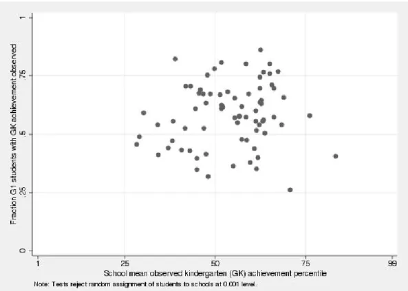
separate. First, a selection process matches students to schools at the beginning of the year. Students are not assigned to schools randomly, so this generates unobserved differences be-tween school populations. Figure 1 gives a sense of how different the Project STAR schools are from one another in terms of average returning student achievement and fraction of students returning. Second, unobserved school quality differences operate during the year. Non-shared, within-school unobserved influences are captured in𝑒∈R with𝐸[𝑒∣𝑠] normalized to 0.

Define 𝜃 ≡ (𝛽, 𝑓, 𝛾) to represent elements of the production function. Neither 𝜃 nor the conditional distribution of individual unobserved influences𝑃(𝑒∣𝑣¯𝑜𝑏,𝑣¯𝑚, 𝑥, 𝑠, 𝑧, 𝑝) is known.

If one assumes that the unobserved influences 𝑒 and the missing 𝑥 values have known parametric distributions and that the𝑥data are missing at random conditional on observable data, one can achieve point identification by integrating out the missing data. Such a model can be estimated by maximum likelihood methods. However, the focus here is on obtaining identification absent these strong assumptions, which have questionable credibility in this application and many others.

spread of peer achievement would be particularly interesting because, for the school principal, moving from a policy of achievement mixing to one of achievement tracking would increase the spread of each student’s peers’ lagged achievement in addition to introducing changes in the peer mean.

3

Identification

This section explores identification of𝜃under various conditions on the peer group formation and data missingness processes. Throughout, we suppose the researcher has an interest in 𝑃(𝑦∣¯𝑣, 𝑥, 𝑠), which is equivalent to knowledge of 𝜃. It describes the distribution of outcomes among students with individual, observable pre-assignment characteristics𝑥who are assigned to a class with peers of type ¯𝑣. This knowledge in the presence of peer effects could help a school principal raise welfare through classroom composition policy. If the principal can take the distribution of students as given and if𝜃captures a stable structural relationship between peers and outcomes, this is all the principal needs. In more general, more realistic contexts, families and schools can respond to one another’s decisions [Epple and Romano (1998), Epple et al. (2002), Hidalgo-Hidalgo (2007), Carrell et al. (2010)]. In that case, knowledge of 𝜃 is useful but not sufficient for optimal policy.

3.1 Complete data, 𝑃 𝑟(𝑧 = 1) = 1

As a prelude to the problem of missing peer data, this section discusses the most common way researchers identify peer effects given complete data. The primary concern is potential selection into peer groups. A mean independence condition identifies𝜃if all data are observed:

𝑀 𝐼:𝐸[𝑒∣𝑣, 𝑥, 𝑠¯ ] =𝐸[𝑒∣𝑠].

Here, the researcher observes𝑃(𝑦,𝑣¯𝑜𝑏_{, 𝑥, 𝑠∣𝑧= 1, 𝑝= 1) =𝑃(𝑦,𝑣, 𝑥, 𝑠¯ ). This implies𝑃(𝑦∣𝑣, 𝑥, 𝑠¯ ),}

which identifies𝜃 under𝑀 𝐼. Mean regression of𝑦 on (¯𝑣𝑜𝑏_{, 𝑥, 𝑠) identifies 𝛽,𝑓, and 𝛾} 𝑠:

𝐸[𝑦∣¯𝑣𝑜𝑏, 𝑥, 𝑠, 𝑧= 1] = 𝐸[𝑦∣¯𝑣, 𝑥, 𝑠]

= 𝛽𝑣¯+𝑓(𝑥) +𝛾𝑠+𝐸[𝑒∣𝑣, 𝑥, 𝑠¯ ]

The credibility of inference hinges on the credibility of 𝑀 𝐼. It overcomes the first method-ological challenge, allowing researchers to separate the causal peer effects of ¯𝑣from the effects of unobserved influences𝑒.

Consider an example when𝑀 𝐼would not be satisfied. Suppose unobserved teacher quality were systematically matched to student achievement and, hence, to peer achievement. This might happen due to unmodeled parent, teacher, or principal influence over the student-teacher matching process. Identification of peer effects will fail, as 𝑒 would not be mean independent of ¯𝑣. Estimates of 𝛽 would suffer from omitted-variable bias. If better teachers go to classes with higher (lower) levels of lagged student achievement, the effect of mean peer lagged achievement will be over- (under) stated.

Random assignment of students and teachers to classes has great value because it gives𝑀 𝐼 credibility. To see this, decompose school unobserved influences into a shared, within-class component and an idiosyncratic component,𝑒≡𝜅𝑐+𝜖. Unobserved differences in teacher

quality or other classroom resources that affect everyone in class equally are captured by𝜅𝑐.

Under random assignment of teachers, expected teacher quality does not depend on own and peer𝑥, 𝐸[𝜅𝑐∣𝑠] = 𝐸[𝜅𝑐∣¯𝑣, 𝑥, 𝑠]. Under random assignment of students,𝐸[𝜖∣𝑣, 𝑥, 𝑠¯ ] = 𝐸[𝜖∣𝑥, 𝑠]

since peer 𝑥 is randomly assigned and independent of own 𝜖. Given 𝐸[𝜖∣𝑥, 𝑠] = 𝐸[𝜖∣𝑠], we obtain𝑀 𝐼.4

In this way, Sacerdote (2001) and Zimmerman (2003) study the effect that randomly-assigned college roommates have on one another. Others have exploited the random as-signment of students and teachers to classes in Project STAR to understand the effect of pre-assignment observables. Dee (2004) studies the effect of student-teacher racial matches, Whitmore (2005) the effect of fraction of peers female, and Cascio and Schanzenbach (2008) the effect of peers’ ages. Unlike the present study, previous papers have not included pre-assignment achievement in own or peer𝑥 because these measures are not generally available in the STAR data.

Boozer and Cacciola (2001) and Graham (2008) also study peer effects using the STAR

4_{Formal arguments are provided in Section A of the Web Appendix available athttps://netfiles.umn.} edu/users/asojourn/Sojourner_Peer_WebApp.pdf.

data, but their work differs from the approach described thus far. One fundamental difference is that they study the effect of peers’𝑦 on own𝑦 rather than the effect of peers’ 𝑥 on own𝑦. This is possible without pre-assignment measures of achievement but is not as useful for the school principal’s problem, since𝑦 is not observable at the time classroom allocations must be decided. Also, methodologically Graham does not use mean independence conditions but develops an innovative analysis based on conditional variance restrictions.

Without random assignment of students and teachers to classes, researchers justify 𝑀 𝐼 in other ways. They may assume that they are conditioning on sufficient observables so as to render unobservables mean independent [Ding and Lehrer (2007)]. Given multiple matches of students and teachers, student and teacher fixed effects can be used to condition out the constant, additive unobserved influences attributable to each [Betts and Zau (2004), Arcidiacono et al. (2007), Burke and Sass (2008)]. However, the credibility of this approach is undermined if schools sort students on the basis of annual fluctuations in unobservables. Rothstein (2010) finds evidence of precisely this in elementary schools. Other researchers appeal to known institutional features of the data-generating process to argue that variation in peer assignment is mean independent of unobservables [Hoxby (2000), Lavy et al. (2007), Vigdor and Nechyba (2007)]. Some papers combine both fixed effects and knowledge of the data-generating process [Hanushek et al. (2003), Cooley (2006), Hoxby and Weingarth (2007), Zabel (2008)]. All of these aim to make𝑀 𝐼 credible without groups being formed by random assignment of students and teachers.

3.2 New approaches given missing data

Consider the common case where each class contains individuals with missing data on the peer-influencing covariate. The researcher observes 𝑃(𝑦,𝑣¯𝑜𝑏, 𝑥, 𝑠, 𝑧, 𝑝) across individuals. Using

equations (1) and (3), the mean regression of𝑦 on (𝑣𝑜𝑏, 𝑝, 𝑥, 𝑠, 𝑧= 1) gives

𝐸[𝑦∣¯𝑣𝑜𝑏, 𝑝, 𝑥, 𝑠, 𝑧= 1] = 𝐸[𝛽[¯𝑣𝑜𝑏𝑝+ ¯𝑣𝑚(1−𝑝)] +𝑓(𝑥) +𝛾𝑠+𝑒∣𝑣¯𝑜𝑏, 𝑝, 𝑥, 𝑠, 𝑧= 1]

= 𝛽𝑣¯𝑜𝑏𝑝+𝛽(1−𝑝)𝐸[¯𝑣𝑚∣𝑣¯𝑜𝑏, 𝑝, 𝑥, 𝑠, 𝑧= 1]

+𝑓(𝑥) +𝛾𝑠+𝐸[𝑒∣¯𝑣𝑜𝑏, 𝑝, 𝑥, 𝑠, 𝑧= 1]. (4)

This regression focuses on the subsample of students whose own 𝑣 is observed (𝑧 = 1). By assuming𝑧does not enter the production function, we imposed that the 𝑧= 1 subpopulation and the whole population share the same𝛽 and𝑓.5 However, the distributions of𝑥and 𝑒can differ depending on 𝑧. Without further conditions, 𝜃 is not identified. We want conditions that overcome two main challenges: selection (the distribution of𝑒depends on (¯𝑣𝑜𝑏, 𝑝, 𝑥)) and

missing data (the distribution of ¯𝑣𝑚depends on (¯𝑣𝑜𝑏, 𝑝, 𝑥)). The following sections study such

conditions.

3.2.1 Mean independence and connection to random assignment of students

This section describes a new way to handle missing peer data relying on two mean indepen-dence conditions,𝑀 𝐼1 and 𝑀 𝐼2, to point-identify 𝛽. Random assignment of students (both those with observed and those with missing𝑣) and teachers to classes helps make these condi-tions credible, but random assignment is not necessary for the condicondi-tions to hold. Beyond this, no other conditions are imposed on the missing data, such as missing completely at random or missing at random conditional on observables. The missing and observed data could come from arbitrarily different distributions, making the analysis consistent with data missing not at random (MNAR) or nonignorability. For example, it could be that students with observed 𝑣 data are higher achieving than those with missing data, so that 𝐸[𝑣𝑜𝑏∣𝑠]> 𝐸[𝑣𝑚∣𝑠].

Sec-tion A of the Web Appendix formally connects the mean independence condiSec-tions to random assignment.

5_{Alternatively, this analysis could be interpreted as identifying the effect of observed peers, which may differ}

from the unidentified effect of missing-data peers. That is, in the last line of equation (4), we could distinguish 𝛽𝑜𝑏 _{as the parameter multiplying ¯𝑣}𝑜𝑏_{𝑝 and 𝛽}𝑚 _{as the parameter on (1−𝑝)𝐸[¯𝑣}𝑚_∣𝑣¯𝑜𝑏_{, 𝑝, 𝑥, 𝑠, 𝑧 = 1]. In the}

The first mean independence condition requires that any student in school-𝑠would expect the mean of her peers’ missing𝑣 (¯𝑣𝑚) to be the same as the average missing 𝑣 in the school regardless of the realized mean𝑣 of the student’s own observed-data peers (¯𝑣𝑜𝑏_{), the fraction}

of her peers with observed𝑣 (𝑝), her own characteristics (𝑥), or the observability of her own 𝑣 (𝑧):

𝑀 𝐼1 :𝐸[¯𝑣𝑚∣¯𝑣𝑜𝑏, 𝑝, 𝑥, 𝑠, 𝑧] =𝐸[𝑣𝑚∣𝑠].

Among students with missing 𝑣 in the school population, there is an average value for 𝑣, 𝐸[𝑣𝑚∣𝑠]. Random assignment of students to classes within school implies the credibility of

𝑀 𝐼1. By random assignment of students to classes, each student in the school should expect her missing peers’ mean𝑣 to equal it. Conditional on school, (¯𝑣𝑜𝑏, 𝑝, 𝑥, 𝑧) does not affect this

expectation. Although random assignment of all individuals to groups is sufficient for𝑀 𝐼1, it is not necessary. 𝑀 𝐼1 can arise under other assignment processes. For instance,𝑀 𝐼1 would also come from a deterministic process of assigning𝑧= 0 individuals to classes in a way that is independent of the assignment of𝑧= 1 individuals (¯𝑣𝑜𝑏, 𝑥, 𝑧= 1) and the fraction of 𝑧= 1

individuals per class, which determines𝑝.6

We also use a mean independence condition on the within-school unobserved influences of those with observed𝑣:

𝑀 𝐼2 :𝐸[𝑒∣¯𝑣𝑜𝑏, 𝑝, 𝑥, 𝑠, 𝑧= 1] =𝐸[𝑒∣𝑠, 𝑧= 1].

Conditional on school and own observability (𝑠, 𝑧= 1), the expected unobserved influence on outcomes is the same for all students regardless of (¯𝑣𝑜𝑏, 𝑝, 𝑥). Random assignment of teachers

gives credibility to 𝜅𝑐 ⊥ (¯𝑣𝑜𝑏, 𝑝, 𝑥). Conditional on (𝑠, 𝑧 = 1), systematic matching of 𝜅𝑐

6_{The following three examples are constructed simply to illustrate that 𝑀 𝐼1 can hold without random}

assignment of all individuals to groups. They do not describe the STAR data. First, suppose𝑧= 1 individuals are randomly assigned to classes. Suppose further that all𝑧= 0 individuals share a single value of𝑥=𝑥𝑚_{. In}

that case, Var(𝑥𝑚) = 0, so ¯𝑣𝑚is constant and𝑀 𝐼1 holds. Second, suppose there are two values of𝑥𝑚: one higher and one lower,𝑥𝑚ℎ_{> 𝑥}𝑚𝑙_{. Suppose a principal knows each 𝑧= 0 student’s value of𝑥}𝑚_{although the}

econometrician does not. If the principal assigns one𝑥𝑚ℎ and one𝑥𝑚𝑙 individual to each class in the school, then𝑀 𝐼1 will hold. Third, suppose that one of each type is assigned to half the classes and two of each are assigned to the other half and that the choice between these two treatments is random; then𝑀 𝐼1 holds. In each case, ¯𝑣𝑚is the same for every student in the school and𝑀 𝐼1 holds. More cases are possible.

to students depending on (𝑣, 𝑥, 𝑝) would violate 𝑀 𝐼2. Systematic matching would create a classic omitted-variable problem. Random assignment of teachers to classes within school alleviates concern about this problem. The same arguments apply to any other influence common within class but differing between classes within schools, such as teachers’ aides or computers. If they are unobserved and mean dependent on observables, they threaten identification. If they are either observed or mean independent of observables, they do not. Random assignment of students to classes ensures that students’ idiosyncratic, unobserved influences 𝜖 are independent of (¯𝑣𝑜𝑏, 𝑝). Given these and a standard mean independence

assumption (𝐸[𝜖∣𝑥, 𝑠, 𝑧 = 1] =𝐸[𝜖∣𝑠, 𝑧= 1]),𝑀 𝐼2 follows.

𝑀 𝐼1−𝑀 𝐼2 are sufficient for point identification of 𝛽. They imply that equation (4) becomes

𝐸[𝑦∣¯𝑣𝑜𝑏, 𝑝, 𝑥, 𝑠, 𝑧= 1] = 𝛽¯𝑣𝑜𝑏𝑝+𝛽(1−𝑝)𝐸[¯𝑣𝑚∣¯𝑣𝑜𝑏, 𝑝, 𝑥, 𝑠, 𝑧 = 1]

+𝑓(𝑥) +𝛾𝑠+𝐸[𝑒∣𝑣¯𝑜𝑏, 𝑝, 𝑥, 𝑠, 𝑧= 1]

= 𝛽¯𝑣𝑜𝑏𝑝−𝛽𝐸[𝑣𝑚∣𝑠]𝑝+𝛽𝐸[𝑣𝑚∣𝑠] +𝑓(𝑥) +𝛾𝑠+𝐸[𝑒∣𝑠, 𝑧= 1].

(5)

The production function (1) and decomposition of ¯𝑣 (3) give the first equality. 𝑀 𝐼1−𝑀 𝐼2 give the second.

Equation (5) is the basic expression used for identification. Consider the mean regression of 𝑦on (¯𝑣𝑜𝑏𝑝, 𝑝⋅1𝑠, 𝑥,1𝑠). Variation in ¯𝑣𝑜𝑏𝑝identifies the peer mean effect𝛽. Variation in𝑝within

school permits recovery of each school’s mean missing𝑣,𝐸[𝑣𝑚∣𝑠], from the second term and

knowledge of𝛽. It is the coefficient on𝑝⋅1𝑠divided by𝛽. This permits identification of𝐸[𝑣𝑚∣𝑠]

as𝑛𝑠→ ∞. The coefficient on each school-𝑠dummy identifies 𝛽𝐸[𝑣𝑚∣𝑠] +𝛾𝑠+𝐸[𝑒∣𝑠, 𝑧= 1],

from which we can back out 𝛾𝑠 +𝐸[𝑒∣𝑠, 𝑧 = 1] ≡ 𝛾1𝑠. Using just the 𝑧 = 1 subsample

yields school fixed effects normalized to their mean unobserved influence. Estimates based on equation (5) will be referred to asp-weight estimators.

𝑀 𝐼1. Conditions such as data MCAR or MAR were not necessary. However, random assign-ment of𝑧= 0 students and the additive separability of ¯𝑣 in individual peer𝑥 were essential. Identification in more general production models is possible but challenging.7

This analysis suggests that mean regression of𝑦𝑠𝑐𝑖 on (¯𝑣𝑠𝑐𝑖𝑜𝑏𝑝𝑠𝑐𝑖, 𝑥𝑠𝑐𝑖, 𝑝𝑠𝑐𝑖1𝑠,1𝑠) conditional

on𝑧𝑠𝑐𝑖= 1 will produce an unbiased estimate of𝛽and other production parameters. However,

in estimation, we are concerned with variance as well as bias. Unfortunately, inclusion of the 𝑝𝑠𝑐𝑖1𝑠 interaction terms induces a great deal of collinearity with other regressors (¯𝑣𝑜𝑏𝑠𝑐𝑖𝑝𝑠𝑐𝑖,1𝑠)

and requires estimation of𝑆 parameters, one for each school, in addition to the production parameters (𝛽, 𝑓, 𝛾).

As interest focuses on𝛽 and we are willing to forego estimation of the𝑆 separate 𝐸[𝑣𝑚∣𝑠] values, we propose a set of restricted estimators, closely related to the unrestricted𝑝-weight estimator. These greatly improve precision at the cost of introducing some bias. Below, we analytically study the bias and propose ways to deal with it. Rather than including𝑆 terms interacting 𝑝 with school fixed effects, consider a model with 𝐾 such interaction terms for 1≤𝐾 < 𝑆. In such a model, the𝑆 schools are partitioned into𝐾 groups, a set of𝐾 dummies are created 1𝑘, and each student’s𝑝 is interacted with her group dummy. The regression of𝑦

on (¯𝑣𝑜𝑏𝑝, 𝑝1𝑘, 𝑥,1𝑠, 𝑧= 1) is studied.

This proposal leads to two practical questions. First, how many groups should be formed? That is, which𝐾 should be used? In simulations and empirical analysis, I present estimates based on a range of 𝐾 from 1 to 𝑆: 1, 3, 15, 25 and 75. The unrestricted estimator has 𝐾=𝑆 = 75. Second, how should the schools be partitioned into groups? In theory, grouping schools with similar missing student means should reduce bias. If schools𝑠 and𝑠′ had equal

7_{Consider replacing𝛽𝑣¯in the production function with the more generalℎ(¯𝑣) =ℎ(¯𝑣}𝑜𝑏_{𝑝+ ¯𝑣}𝑚_{(1−𝑝)). What}

property ofℎdelivers point identification ofℎwith𝑀 𝐼1? Linearity. Mathematically, it allows the expectation operator to pass inside the function and to separate the missing and observed components. Substantively, it says that variation in the observed portion is sufficient to identify a peer effect.

Consider studying the effect of other properties of the peer𝑣distribution besides the mean, ¯𝑣. A different issue arises. Although random assignment guarantees that the expectation of ¯𝑣 is constant within a school regardless of the number of missing-data students in a class, the same is not true for the expectation of other properties of the peer𝑣 distribution. For instance, the variance of mean missing peer 𝑣𝑚 _{depends on the}

number of𝑧 = 0 students whose𝑣𝑚 are being averaged to form ¯𝑣𝑚. Therefore, across classes with different numbers of missing-data students, the variance of ¯𝑣𝑚 _{will not be constant. This can be dealt with using}

missing data means (𝐸[𝑣𝑚∣𝑠] =𝐸[𝑣𝑚∣𝑠′]), equation (5) shows that grouping them would create

no bias and would reduce variance. However,𝐸[𝑣𝑚∣𝑠] are never observed. Assumptions about the relationship between observables and 𝐸[𝑣𝑚_{∣𝑠] can be used. For instance, assume that}

the missing student mean and observed student mean have the same rankings across schools: 𝐸[𝑣𝑜𝑏∣𝑠]< 𝐸[𝑣𝑜𝑏∣𝑠′]⇒𝐸[𝑣𝑚∣𝑠]< 𝐸[𝑣𝑚∣𝑠′]. This suggests partitioning the schools into groups

on the basis of their observed student mean𝑣rankings — dividing them into 𝐾-ciles. If true, this should lead to less bias than some other partitions into𝐾 groups.

To understand the bias of these estimators, consider the limiting case where no group dummy×𝑝terms are included (𝐾= 0). Transforming to first differences permits a relatively simple expression for bias in this case. Define 𝑤∗ as the difference between any variable 𝑤=𝑦,𝑣¯𝑜𝑏_{𝑝, 𝑝, 𝑒and its expectation conditional on (𝑥,1}

𝑠, 𝑧 = 1): 𝑤∗ ≡𝑤−𝐸[𝑤∣𝑥, 𝑠, 𝑧 = 1].

Then,

𝑦∗ =𝛽𝑣¯𝑜𝑏𝑝∗+𝛽𝐸[𝑣𝑚∣𝑠]𝑝∗+𝑒∗

The bias in estimating 𝛽 by regression of 𝑦∗ on ¯𝑣𝑜𝑏𝑝∗ is the covariance of the regressor with

the omitted terms𝐸[𝑣𝑚∣𝑠]𝑝∗ over the variance of the regressor,

𝛽X 𝑠

𝐸[𝑣𝑚∣𝑠]𝐸[1𝑠(¯𝑣

𝑜𝑏_𝑝∗_)(𝑝∗_)]

𝑉(¯𝑣𝑜𝑏_𝑝∗₎ . (6)

In this case, bias increases in𝛽,𝐸[𝑣𝑚∣𝑠], and𝐸[1𝑠(¯𝑣𝑜𝑏𝑝∗)(𝑝∗)]. It decreases in𝑉(¯𝑣𝑜𝑏𝑝∗). This

is analogous to a panel data model where there is a common main effect of an interaction of two variables and a unit-specific effect of one of the variables.

Monte Carlo simulations can compare the performance of𝑝-weight estimators with various 𝐾 to one another and to the two other estimators in the literature — the IDP and AP-corrected IDP — in terms of bias, variance, and mean squared error (MSE).8 We consider four different data-generating processes (DGP). In every DGP, observed data are taken as given, values for the missing𝑣𝑚 data are drawn for each 𝑧= 0 student from a school-specific

distribution, and outcomes are generated. Then the generated𝑣𝑚 data are deleted and peer

8_{The IDP and AP-corrected IDP will be discussed analytically in Section 3.3; discussion of the simulation}

effects are estimated. DGP vary along two dimensions: how the ordering of schools’ missing student mean lagged achievement𝐸[𝑣𝑚∣𝑠] was determined and whether teachers (correlated effects) are absent/present. For each DGP, 5,000 Monte Carlo replications were performed. In each replicate, all seven estimators were used to estimate 𝛽. The distribution of each estimator’s 5,000 ˆ𝛽s measure its squared error, variance, and MSE.

Monte Carlo results are presented in Table 1. Each estimator’s MSE is expressed as a multiple of the MSE for the unrestricted𝑝-weight estimator in the no-teacher condition under the same𝐸[𝑣𝑚∣𝑠]-ordering process. The share of each estimator’s total MSE due to squared

error and to variance is also displayed.

What do the results tell us about the performance of the𝑝-weight estimators with various 𝐾? Consider the top left panel where the assumption that the missing student mean and ob-served student mean have the same rankings across schools (𝐸[𝑣𝑜𝑏∣𝑠]< 𝐸[𝑣𝑜𝑏∣𝑠′]⇒𝐸[𝑣𝑚∣𝑠]<

𝐸[𝑣𝑚∣𝑠′]) is true. As expected, the unrestricted𝑝-weight estimator appears unbiased. Squared

error accounts for only 0.02 percent of the MSE whereas variance accounts for the other 99.98 percent. The MSE of the restricted𝑝-weight estimators is less for all𝐾. Bias does not appear to be a problem, but reducing the collinearity in the regressors and reducing the number of parameters estimated does reduce variance considerably. Including randomly assigned teach-ers raises the variance of all the estimators but does not affect bias. For instance, the MSE of the unrestricted 𝑝-weight estimator is 1.56 times larger when teachers are included as when they are excluded.

What happens if our assumption about the ranking of schools’ 𝐸[𝑣𝑚∣𝑠] is violated? The

right panel of Table 1 assigns𝐸[𝑣𝑚∣𝑠] randomly while ensuring that they have similar

distri-butional characteristics as obtained in the other DGP. Relative performance does not change much, although the variance of all estimators increases. The unrestricted 𝑝-weight estima-tor in the no-teacher condition has an MSE that is 17.4 times larger in the random ranking condition than in the𝐸[𝑣𝑜𝑏∣𝑠] ordering condition. The MSE decreases proportionally less as

𝐾 decreases and increases more when teachers are considered. However, in every case, bias remains minimal. Shifting the𝐸[𝑣𝑚∣𝑠] to extreme values does increase bias considerably for

𝐾 < 𝑆 but not for𝐾 =𝑆, as expected from equation (6) (results available on request).

3.2.2 Analyzing students with missing 𝑥 data

Thus far, we have ignored outcome and available covariate information for students with missing data on a peer-influencing covariate (𝑧 = 0). This section extends𝑝-weight analysis to those with 𝑧 = 0 using a few mild assumptions. Although some components of 𝑥 are sometimes missing, other components are always observed. Divide the components of 𝑥 between those that are sometimes missing (𝑎) and those that are always observed (𝑏) such that𝑥≡(𝑎′, 𝑏′)′.

We can use the observed (𝑦, 𝑏∣𝑧 = 0) information to estimate 𝛽 by studying the effect of observed peer mean on outcomes among those with𝑧= 0. Although we cannot condition on𝑎 for these students, random assignment ensures that observed peer quality is mean independent of observed characteristics and therefore delivers an unbiased estimate of peer effects. With nonparametric𝑓, no new structure is required. For linear 𝑓(𝑎, 𝑏), the expectation of 𝑎must be linear in𝑏: 𝐸[𝑎∣𝑏, 𝑠, 𝑧= 0]≡𝛿𝑎(see note for details).9 We can combine the analysis done

9_{Let a new conditioning set be ˜𝑑≡(¯𝑣}𝑜𝑏_{, 𝑝, 𝑏, 𝑠, 𝑧 = 0). Assume two mean independence conditions closely}

linked to those defined earlier and one new one. These are formally justified in Section A of the Web Appendix.

𝑀 𝐼1𝑏: 𝐸[¯𝑣𝑚∣𝑣¯𝑜𝑏, 𝑝, 𝑏, 𝑠, 𝑧= 0] =𝐸[𝑣𝑚∣𝑠]

𝑀 𝐼2𝑏: 𝐸[𝑒∣𝑣¯𝑜𝑏, 𝑝, 𝑏, 𝑠, 𝑧= 0] =𝐸[𝑒∣𝑠, 𝑧= 0]

𝑀 𝐼3𝑏: 𝐸[𝑓(𝑎, 𝑏)∣𝑣¯𝑜𝑏, 𝑝, 𝑏, 𝑠, 𝑧= 0] =𝐸[𝑓(𝑎, 𝑏)∣𝑏, 𝑠, 𝑧= 0]

Their credibility depends on random assignment. 𝑀 𝐼1𝑏 follows directly from𝑀 𝐼1. 𝑀 𝐼2𝑏 is justified by the

same logic as𝑀 𝐼2. Neither one’s observed peer mean, fraction of peers observed, own characteristics, nor unobserved teacher characteristics affect either the expectation of one’s missing peer mean ¯𝑣𝑚or within-school unobserved influences.

𝑀 𝐼3𝑏 is a different kind of condition. It requires that the expected effect of one’s own (𝑎, 𝑏) does not vary

with the realized mean among one’s observed peers ¯𝑣𝑜𝑏 _{or the fraction𝑝of observed peers. It deals with the}

expected effect of𝑓(𝑎, 𝑏) on 𝑦where 𝑓(𝑎, 𝑏) is integrated over the distribution of (𝑎, 𝑏) conditional on ˜𝑑. In the production function, (𝑎, 𝑏) does not interact with ¯𝑣𝑜𝑏 _{or𝑝, so that the productivity of own (𝑎, 𝑏) does not}

change with (¯𝑣𝑜𝑏, 𝑝). By random assignment,𝑃(𝑎, 𝑏∣¯𝑣𝑜𝑏, 𝑝, 𝑏, 𝑠, 𝑧= 0) =𝑃(𝑎, 𝑏∣𝑏, 𝑠, 𝑧= 0).These imply𝑀 𝐼3𝑏.

Taking the expectation of the production equation conditional on ˜𝑑gives

𝐸[𝑦∣𝑑˜] = 𝛽𝑣¯𝑜𝑏𝑝+𝛽𝐸[¯𝑣𝑚(1−𝑝)∣𝑑˜] +𝐸[𝑓(𝑎, 𝑏)∣𝑑˜] +𝛾𝑠+𝐸[𝑒∣𝑑˜]

= 𝛽𝑣¯𝑜𝑏𝑝+𝛽𝐸[𝑣𝑚∣𝑠]−𝛽𝐸[𝑣𝑚∣𝑠]𝑝+𝐸[𝑓(𝑎, 𝑏)∣𝑏, 𝑠, 𝑧= 0] +𝛾𝑠+𝐸[𝑒∣𝑠, 𝑧= 0].

The first term identifies𝛽. The covariates 𝑏 no longer identify 𝑓. They pick up a mix of direct effects of 𝑏 and indirect effects of 𝑎 correlated with 𝑏. For instance, suppose 𝑓 is additively separable in 𝑎 and 𝑏: 𝑓(𝑎, 𝑏)≡𝑓𝑎(𝑎) +𝑓𝑏(𝑏). Then variation in𝑏identifies𝐸[𝑓𝑎(𝑎)∣𝑏, 𝑠, 𝑧= 0] +𝑓𝑏(𝑏). The other terms work as in

Section 3.2.1. For linear𝑓(𝑎, 𝑏)≡𝜋𝑎𝑎+𝜋𝑏𝑏, which is used in estimation, the conditional expectation of𝑎must

on 𝑧 = 0 and 𝑧 = 1 students into one analysis. In practice, this is implemented in a single regression with appropriate interactions with𝑧.

Thus far, we have not pursued the traditional route for dealing with missing data, which is to impose some equivalence across the distributions of (𝑥, 𝑒) between students with 𝑧= 1 and𝑧 = 0 such as MCAR or MAR. Everything has been done in a way consistent with data missing not at random (MNAR). In the application, this approach seems appropriate. The following section proposes a new method for improving inference under stronger assumptions.

3.2.3 Improving inference with information about variance ratios

This section develops conditions that allow use of observed differences across classes in the missing-data students’ outcomes (𝑦) and never-missing covariates (𝑏) to make inference about differences across classes in the average missing peer-influencing variables ¯𝑣𝑚. This brings

more information to bear in making inference about𝛽. The variables used are the same as in the previous section, but now (𝑦, 𝑏) conditional𝑧= 0 are taken as informative about the class’s ¯

𝑣𝑚, whereas the only structure imposed on ¯𝑣𝑚 until now was𝑀 𝐼1. New structure is assumed, which tightens inference. The approach borrows from the measurement error literature [Boggs et al. (1987), Carroll (2006)] and exploits information about the ratio between the variance of 𝜖for any𝑧= 1 student and the variance of the average𝜖among all missing-data students in the same class. This information depends on the assumption that𝑧= 1 and𝑧= 0 students’𝜖 come from distributions with the same variance conditional on observables. Such conditions provide a new way to identify peer effects in the presence of missing data that may be useful in many settings.

The study of peer effects provides a uniquely credible setting for using this variance ratio approach to measurement error because, here, one student’s outcome error𝑒is the source of other students’ measurement error in covariates. In contrast, in most settings outside social interactions, measurement error derives from a source less closely related to the outcome error. Recast the missing peer mean ¯𝑣𝑚 in terms of average observables and unobservables by

Con-sider any class-𝑐. It has𝑁𝑐students: 𝑛𝑐with𝑧= 1 and𝑁𝑐−𝑛𝑐students with𝑧= 0. Define the

average value among missing-data students in the class as𝑤𝑠𝑐0 ≡(𝑁𝑐−𝑛𝑐)−1

P

𝑖∈𝑐𝑤𝑠𝑐𝑖(1−𝑧𝑠𝑐𝑖)

for any variable 𝑤 = 𝑦, 𝑎, 𝑏, 𝑝,¯𝑣𝑜𝑏_{𝑝, 𝑒. This is a class average conditional on 𝑧}

𝑠𝑐𝑖 = 0, not a

leave-me-out mean.

We use two new assumptions about functional form. First, assume production is linear (𝑓(𝑎, 𝑏) ≡𝜋𝑎𝑎+𝜋𝑏𝑏). Second, assume peer effects operate through 𝑎≡𝑣 = 𝑔(𝑎, 𝑏); that is,

we want to study the effect of the average value of the sometimes-missing, peer-influencing variable per se rather than a known function of it.

It follows that for any 𝑧 = 1 student, her missing peer mean — the vexing variable that causes all the trouble — can be expressed as

¯ 𝑣𝑚_𝑠𝑐𝑖= 𝑦𝑠𝑐0−𝛽¯𝑎 𝑜𝑏_𝑝 𝑠𝑐0−𝜋𝑏𝑏𝑠𝑐0−𝛾𝑠−𝑒𝑠𝑐0 𝛽(1−𝑝_𝑠𝑐0) +𝜋𝑎 (7) .

Details are available.10

10_{Consider any student-𝑗with𝑧}

𝑠𝑐𝑗= 0. They all share the same values of variables relating to one’s

observed-data peers. The fraction of 𝑗’s peers with 𝑧 = 1 is 𝑝𝑠𝑐𝑗 = 𝑁𝑐_𝑁−𝑛𝑐−1

𝑐−1 =𝑝𝑐0, and the observed peer mean is ¯

𝑣𝑜𝑏

𝑠𝑐𝑗= ¯𝑣𝑜𝑏𝑐0. Their product is ¯𝑣𝑠𝑐𝑗𝑜𝑏 𝑝𝑠𝑐𝑗= ¯𝑣𝑜𝑏𝑝𝑠𝑐0.

For any class-𝑐, the𝑧 = 1 students’ missing peer mean, which is the average𝑣=𝑎 of the𝑧 = 0 students in class-𝑐, can be expressed as a function of observable characteristics of 𝑧= 0 students and other factors by manipulating the𝑧= 0 students’ production equations. The production model implies that, for any𝑗,

𝑦𝑠𝑐𝑗 = 𝛽𝑣¯𝑜𝑏𝑠𝑐𝑗𝑝𝑠𝑐𝑗+𝛽𝑣¯𝑠𝑐𝑗𝑚(1−𝑝𝑠𝑐𝑗) +𝜋𝑎𝑎𝑠𝑐𝑗+𝜋𝑏𝑏𝑠𝑐𝑗+𝛾𝑠+𝑒𝑠𝑐𝑗 = 𝛽𝑣¯𝑜𝑏_𝑝 𝑠𝑐0+𝛽[(𝑁𝑐−𝑛𝑐−1)−1 X 𝑘∕=𝑗,𝑧𝑠𝑐𝑘=0 𝑎𝑚𝑠𝑐𝑘](1−𝑝𝑠𝑐0) +𝜋𝑎𝑎𝑠𝑐𝑗+𝜋𝑏𝑏𝑠𝑐𝑗+𝛾𝑠+𝑒𝑠𝑐𝑗. (8)

Indexing the𝑧= 0 individuals in class-𝑐by𝑗= 1,2...(𝑁𝑐−𝑛𝑐) and adding up their production equations (8)

gives X 𝑗 𝑦𝑠𝑐𝑗= (𝑁𝑐−𝑛𝑐)𝛽𝑣¯𝑜𝑏𝑝𝑠𝑐0+𝛽(1−𝑝𝑠𝑐0) X 𝑗 𝑎𝑚𝑠𝑐𝑗+𝜋𝑎 X 𝑗 𝑎𝑚𝑠𝑐𝑗+𝜋𝑏 X 𝑗 𝑏𝑠𝑐𝑗+ (𝑁𝑐−𝑛𝑐)𝛾𝑠+ X 𝑗 𝑒𝑠𝑐𝑗. (9) The𝑎𝑠𝑐𝑗 in the𝜋𝑎 P 𝑗𝑎 𝑚

𝑠𝑐𝑗 term are all missing since these are𝑧= 0 students. They are the same values in

the𝛽(1−𝑝𝑠𝑐0)

P

𝑗𝑎 𝑚

𝑠𝑐𝑗 term. Any of the𝑧= 1 students will have ¯𝑣𝑚𝑠𝑐𝑖= (𝑁𝑐−𝑛𝑐)−1

P

𝑗∈𝑐,𝑧𝑠𝑐𝑗=0𝑎

𝑚

𝑠𝑐𝑗. Solving

equation (9) for this term yields

(𝑁𝑐−𝑛𝑐)−1 X 𝑗∈𝑐,𝑧𝑠𝑐𝑗=0 𝑎𝑚𝑠𝑐𝑗 = 𝑦𝑠𝑐0−𝛽𝑣¯𝑜𝑏𝑝𝑠𝑐0−𝜋𝑏𝑏𝑠𝑐0−𝛾𝑠−𝑒𝑠𝑐0 𝛽(1−𝑝_𝑠𝑐0) +𝜋𝑎 . (10)

This can be substituted into the production function for 𝑧 = 1 students in class-𝑐 and 𝑒 expanded such that

𝑦𝑠𝑐𝑖 = 𝛽𝑣¯𝑠𝑐𝑖𝑜𝑏𝑝𝑠𝑐𝑖+𝛽𝑣¯𝑠𝑐𝑖𝑚(1−𝑝𝑠𝑐𝑖) +𝜋𝑎𝑎𝑠𝑐𝑖+𝜋𝑏𝑏𝑠𝑐𝑖+𝛾𝑠+𝑒𝑠𝑐𝑖 = 𝛽¯𝑎𝑜𝑏_𝑠𝑐𝑖𝑝𝑠𝑐𝑖+𝛽 – 𝑦_𝑠𝑐0−𝛽¯𝑎𝑜𝑏_𝑠𝑐0𝑝_𝑠𝑐0−𝜋𝑏¯𝑏𝑠𝑐0−𝛾𝑠−𝜅𝑐−𝜖𝑐0 𝛽(1−𝑝_𝑠𝑐0) +𝜋𝑚 ™ (1−𝑝𝑠𝑐𝑖) +𝜋𝑎𝑎𝑠𝑐𝑖+𝜋𝑏𝑏𝑠𝑐𝑖+𝛾𝑠+𝜅𝑐+𝜖𝑠𝑐𝑖. (11)

This single equation captures the relationship between all observable information given the model.

Straight forward estimation based on equation (11) runs into stumbling blocks. Consider the mean regression of 𝑦𝑠𝑐𝑖 on ˇ𝑑 ≡ (¯𝑎𝑜𝑏𝑠𝑐𝑖𝑝𝑠𝑐𝑖, 𝑦𝑠𝑐0,𝑎¯𝑜𝑏𝑝𝑠𝑐0, 𝑏𝑠𝑐0, 𝑎𝑠𝑐𝑖, 𝑏𝑠𝑐𝑖,1𝑠, 𝑧 = 1). For each

𝑧 = 1 student, there are two kinds of unobservables here: additive equation error 𝜅𝑐+𝜖𝑠𝑐𝑖

and measurement error in the covariates expressed in the−𝜅𝑐−𝜖𝑐0 term.

By rearranging equation (7), the measurement error can be expressed as classical, additive error where the noisy measure (the LHS) equals a ratio of the latent true value (¯𝑣𝑚_𝑠𝑐𝑖) plus

noise (𝜅𝑐+𝜖𝑠𝑐0) that has conditional mean zero:

𝑦_𝑠𝑐0+𝛽¯𝑎𝑜𝑏_𝑝

𝑠𝑐0+𝜋𝑏𝑏𝑠𝑐0+𝛾𝑠= [𝛽(1−𝑝𝑠𝑐0) +𝜋𝑎]¯𝑣𝑠𝑐𝑖𝑚 +𝜅𝑐+𝜖𝑠𝑐0.

The measurement error and the equation error in equation (11) are correlated through𝜅𝑐.

This causes problems. One could simply assume that no group-level unobserved influences are present: 𝜅𝑐 ≡ 0. This is not credible in the current application, but it is credible in

some settings. If this assumption is maintained in error, estimates of𝛽 are upwardly biased. Correlation in𝑦𝑠𝑐𝑖and𝑦𝑠𝑐0 would be mistaken for the effect of peers rather than for the effect

of teachers.11

One approach to white-noise measurement error uses a restriction on the ratio of vari-ances between the error in the outcome (𝜖𝑠𝑐𝑖) and the measurement error in the regressor

11

(¯𝜖𝑠𝑐0) [Boggs et al. (1987), Carroll (2006)]. Assume that conditional within-class idiosyncratic

influences for individuals in the same class all have the same variance and are independent across individuals:

𝑉[𝜖∣𝑎¯𝑜𝑏, 𝑝, 𝑎, 𝑏, 𝑐] =𝑉[𝜖∣¯𝑎𝑜𝑏, 𝑝, 𝑎, 𝑏, 𝑐, 𝑧]. (12)

Given random assignment of individuals to classes from school populations, this would follow from 𝑉[𝜖∣𝑠] = 𝑉[𝜖∣𝑧, 𝑠]. Alternatively, it would also follow from the more general missing at random (MAR) assumption: 𝑃[𝜖∣¯𝑎𝑜𝑏, 𝑝, 𝑎, 𝑏, 𝑐] =𝑃[𝜖∣¯𝑎𝑜𝑏, 𝑝, 𝑎, 𝑏, 𝑐, 𝑧]. Then, for any 𝑧= 1 individual in class-𝑐,

𝑉[𝜖𝑠𝑐𝑖∣𝑑ˇ] 𝑉[𝜖𝑠𝑐0∣𝑑ˇ]

=𝑁𝑐−𝑛𝑐. (13)

The ratio of the outcome variance to the measurement error variance is exactly the number of missing-data individuals in the class, that is, the number of individuals over whom the average ¯

𝜖𝑠𝑐0 is taken.12 Averaging over more 𝑧 = 0 students reduces the variance of ¯𝜖𝑠𝑐0 and raises

the ratio. Under this condition, Boggs et al. (1987) develop an estimator based on nonlinear orthogonal regression. Adapted here, we propose to find the parameters that minimize,

min

𝜃,𝜖𝑠𝑐0

Σ𝑧𝑠𝑐𝑖=1[(ˆ𝜖𝑠𝑐𝑖)

2_{+ (𝑁}

𝑐−𝑛𝑐)(𝜖𝑠𝑐0)2],

where ˆ𝜖𝑠𝑐𝑖 is defined as a function of data and parameters after solving equation (11) for𝜖𝑠𝑐𝑖

and 𝜖𝑠𝑐0 is a parameter shared by all 𝑧= 1 students in class-𝑐. This can be implemented by

Generalized Method of Moments. This approach, assuming 𝜅𝑐 ≡ 0, is implemented in the

Section 5 but likely exaggerates peer effects.

3.3 Analysis of and comparison to existing approaches

Boucher et al. (2010) extend the analysis of Lee (2007) to deal with missing data when group-level fixed effects are used. They point out that these fixed effects absorb the influence of

12

More generally, one could assume that 𝜆𝑉[𝜖∣𝑐, 𝑧 = 1] = 𝑉[𝜖∣𝑐, 𝑧 = 0] with a known𝜆. The (equation error/measurement error) ratio would then be𝜆(𝑁𝑐−𝑛𝑐).

missing-data peers as well as teachers or other contextual factors in analysis of the 𝑧 = 1 sample. In the notation here, such a fixed effect would be 𝛾𝑐 ≡ 𝜅𝑐+𝛽¯𝑣𝑚(1−𝑝). Rather

than use across-group variation in peers, this approach identifies peer effects from within-group peer variation derived from leaving 𝑖 out of the class mean 𝑣 for different 𝑖. It uses a mean independence condition similar to 𝑀 𝐼 defined at the class rather than school level. However, in the present application, this approach yields imprecise estimates as class fixed effects explain 99 percent of the variance in ¯𝑣𝑜𝑏.

The most common approach to missing data in the literature is to use an individual-deletion procedure (IDP). This approach produces biased and inconsistent estimates in the presence of missing data. In general the bias can be up or down or can even produce the wrong sign. When individuals are randomly assigned to groups, the bias attenuates estimates to zero. It acts similarly to white-noise measurement error, although it is not exactly that. The best approach in the literature is the correction to the IDP estimator proposed by Ammermueller and Pischke (2009). Its properties relative to 𝑝-weight estimators are explored analytically and through Monte Carlo simulation.

An IDP amounts to regressing𝑦 on (¯𝑣𝑜𝑏, 𝑥,1𝑠) in the𝑧= 1 subsample. For compactness,

let the IDP conditioning variables be represented by a vector𝑑≡(¯𝑣𝑜𝑏, 𝑥′, 𝑠, 𝑧 = 1)′. An IDP

leads one to study the following misspecified regression equation in the𝑧= 1 subpopulation:

𝐸[𝑦∣𝑑] =𝛼𝑣¯𝑜𝑏+𝑓𝐼𝐷𝑃(𝑥) +𝛼𝑠+𝐸[𝑒∣𝑑]. (14)

The peer effect measured by IDP is how the expectation of𝑦 changes as ¯𝑣𝑜𝑏 changes. The

misspecification means that the coefficient on ¯𝑣𝑜𝑏is not constant. It varies with the particular values (¯𝑣𝑜𝑏_{, 𝑥, 𝑠) at which the expression is evaluated. For this reason, it is denoted𝛼(𝑑):}

𝛼(𝑑) = ∂𝐸[𝑦∣𝑑] ∂𝑣¯𝑜𝑏 = 𝛽 𝐸[𝑝∣𝑑] + ¯𝑣𝑜𝑏∂𝐸[𝑝∣𝑑] ∂𝑣¯𝑜𝑏 + ∂𝐸[¯𝑣𝑚∣𝑑] ∂𝑣¯𝑜𝑏 − ∂𝐸[¯𝑣𝑚𝑝∣𝑑] ∂¯𝑣𝑜𝑏 +∂𝐸[𝑒∣𝑑] ∂𝑣¯𝑜𝑏 ≡ 𝛽Λ(𝑑) +∂𝐸[𝑒∣𝑑] ∂𝑣¯𝑜𝑏 . (15)

The ˆ𝛼that is estimated using an IDP is a weighted average of this quantity across values of𝑑. By equation (15), ˆ𝛼 →𝛽 only if ∂𝐸[𝑒∣¯𝑣𝑜𝑏_∂¯𝑣,𝑥,𝑠,𝑧𝑜𝑏 =1] = 0 and Λ(𝑑) = 1 for all (¯𝑣𝑜𝑏, 𝑥, 𝑠) such that

𝑃 𝑟(¯𝑣𝑜𝑏_{, 𝑥, 𝑠, 𝑧 = 1)>0. In general, Λ(𝑑) can take any value. The IDP estimator ˆ𝛼 aggregates}

across estimates of𝛼(𝑑), none of which equal𝛽.

Therefore, the IDP estimator is biased and inconsistent without a general direction, sign, or magnitude. The bias depends on the interaction of the missingness and group formation processes as expressed in Λ(𝑑). Asymptotically, the IDP estimate could be larger or smaller than the true parameter or of an opposite sign. Caution is in order when interpreting IDP estimates in the literature.

We now study how an IDP performs assuming that students are assigned randomly to classes. As before, random assignment implies that errors are mean independent of ¯

𝑣𝑜𝑏 (∂𝐸[𝑒∣𝑣¯_∂𝑜𝑏_¯𝑣,𝑥,𝑠,𝑧𝑜𝑏 =1] = 0) and helps separate causal from correlated effects. However,

ran-dom assignment also ensures that Λ(𝑑) < 1 and that the IDP estimator is attenuated to zero. Under random assignment of students to classes, any student’s 𝑝 will be inde-pendent of her (¯𝑣𝑜𝑏,𝑣¯𝑚, 𝑥) conditional on (𝑧 = 1, 𝑠). This gives both ∂𝐸_∂𝑣¯[𝑝𝑜𝑏∣𝑑] = 0 and ∂𝐸[¯𝑣𝑚_𝑝∣𝑑]

∂𝑣¯𝑜𝑏 =

∂𝐸[¯𝑣𝑚_∣𝑑]

∂¯𝑣𝑜𝑏 𝐸[𝑝∣𝑑]. Further, random assignment implies that the likelihood of any

student’s missing peer mean ¯𝑣𝑚 taking a particular value is independent of (¯𝑣𝑜𝑏, 𝑥, 𝑧)

condi-tional on𝑠. This can be expressed as a mean independence condition that follows from 𝑀 𝐼1, one that excludes 𝑝 from the conditioning set: 𝐸[¯𝑣𝑚∣¯𝑣𝑜𝑏, 𝑥, 𝑠, 𝑧] = 𝐸[𝑣𝑚∣𝑠], which implies

∂𝐸[¯𝑣𝑚∣𝑑] ∂¯𝑣𝑜𝑏 = 0. Therefore, Λ𝑅𝐴(𝑑) = 𝐸[𝑝∣𝑑] + ¯𝑣𝑜𝑏 ∂𝐸[𝑝∣𝑑] ∂𝑣¯𝑜𝑏 + ∂𝐸[¯𝑣𝑚∣𝑑] ∂¯𝑣𝑜𝑏 − ∂𝐸[¯𝑣𝑚𝑝∣𝑑] ∂¯𝑣𝑜𝑏 = 𝐸[𝑝∣𝑑] + (1−𝐸[𝑝∣𝑑])∂𝐸[¯𝑣 𝑚_∣𝑑] ∂¯𝑣𝑜𝑏 = 𝐸[𝑝∣¯𝑣𝑜𝑏, 𝑥, 𝑠, 𝑧 = 1] = 𝐸[𝑝∣𝑠, 𝑧= 1]<1. (16)

The first equality is the definition of Λ(𝑑), the second comes from the independence of 𝑝 and (¯𝑣𝑜𝑏,𝑣¯𝑚, 𝑥), the third from the definition of 𝑑 and ∂𝐸_∂[¯𝑣_𝑣¯𝑚𝑜𝑏∣𝑑] = 0, and the last from the

independence of𝑝 from (¯𝑣𝑜𝑏, 𝑥) conditional on 𝑠. The inequality comes from the presence of

missing data in each class.

Random assignment of students within school makes Λ𝑅𝐴(𝑑) invariant within school.

Us-ing equations (15) and (16), we can define 𝛼𝑅𝐴(𝑑) = 𝛽𝐸[𝑝∣𝑠, 𝑧 = 1] ≡ 𝛼𝑅𝐴(𝑠) < 𝛽. Given

finitely many students and classes per school while allowing the number of schools to go to infinity, the IDP estimator aggregates across schools with different 𝐸[𝑝∣𝑠, 𝑧 = 1]. No 𝐸[𝑝∣𝑠, 𝑧= 1] is identified. The IDP estimator of peer effects ˆ𝛼𝑅𝐴 aggregates across the

sam-ple. Given infinitely many classes in a school-𝑠,𝛽 could be identified using only information from within school-𝑠. As𝑛𝑠→ ∞,𝐸[𝑝∣𝑠, 𝑧= 1] would be observed and𝛽 would be identified

from the IDP as𝛼𝑅𝐴(𝑠)(𝐸[𝑝∣𝑠, 𝑧= 1])−1.

Monte Carlo simulations contrast the properties of the biased, precise IDP estimator and the unbiased, imprecise unrestricted𝑝-weight estimator developed in Section 3.2.1. In these simulations, various fractions of the simulated 𝑎values are then censored.13 Peer effects are estimated using both IDP and 𝑝-weights. Results are displayed in Figure 2. The IDP esti-mates grow more attenuated as the fraction of missing data grows. The𝑝-weight estimator’s confidence intervals contain the true value for all degrees of missingness, but it is imprecise.

Ammermueller and Pischke (2009), through a different route of analysis, arrive at a similar finding and propose a correction to the IDP estimator. They suggest multiplying the IDP estimate by 𝐶−1P_𝑐𝑁𝑐−1

𝑛𝑐−1. Conceptually, this correction factor is very similar to (𝐸[𝑝∣𝑠, 𝑧 =

1])−1_{. Approximately, the AP correction scales up the IDP’s point estimate and standard}

errors by the inverse of the fraction of data observed.

Returning to Table 1, we can compare the performance of the IDP and AP-corrected estimators with that of the𝑝-weight estimators. This evidence illustrates the analytic points made above and shows that across a range of DGP, the restricted 𝑝-weight estimators have minimal bias and reduced variance. Together this translates into lower mean squared error than the alternatives. As expected, the IDP estimator is biased but precise. Its MSE is 51.85 percent that of the unrestricted𝑝-weight estimator but larger than that of all the restricted

13_{In the Table 1 simulation, in contrast, all simulated𝑎values were subsequently censored so that the fraction}

𝑝-weight estimators. Unlike the𝑝-weight estimators, squared error makes a large contribution to the IDP’s MSE. The AP correction generally has a smaller MSE than the unrestricted 𝑝-weight estimator but larger than the MSE of any of the restricted versions. It also has a larger MSE than the IDP estimator. It is much less biased but also much less precise.

The problem with IDP estimates should not be confused with a classical errors-in-variables problem where the observed variable is the true variable plus mean zero noise. To see this, express the noisy observed variable ¯𝑣𝑜𝑏 as a function of the true causal variable ¯𝑣 plus noise.

Rearranging the decomposition of ¯𝑣 gives

¯ 𝑣𝑜𝑏= 1 𝑝¯𝑣+ 1−𝑝 𝑝 𝑣¯ 𝑚

Conditional on any true ¯𝑣 and any 𝑝∈(0,1), the expectation of ¯𝑣𝑜𝑏 is

𝐸[¯𝑣𝑜𝑏∣𝑣¯] = 1 𝑝¯𝑣+

1−𝑝 𝑝 𝐸[¯𝑣

𝑚_∣¯𝑣]

By definition, the noise is mean zero if 𝐸[¯𝑣𝑜𝑏∣𝑣¯] = ¯𝑣. This requires 𝐸[¯𝑣𝑚∣¯𝑣] = ¯𝑣. With-out some further restriction on the distributions of 𝑣𝑜𝑏 _{and 𝑣}𝑚_{, this will not hold. Even if}

𝐸[𝑣𝑚∣𝑠] = 𝐸[𝑣𝑜𝑏∣𝑠], finite sample variance ensures the equality does not hold generally since

the realized ¯𝑣∕=𝐸[𝑣∣𝑠].

3.3.1 Partial identification with data not missing at random

We have explored how a condition on the peer group formation process, random assignment, gives point identification of 𝛽 without requiring conditions on the data missingness process. The identifying power of the random assignment condition can be illustrated by relaxing it and seeing what we learn from the model and the observable data in its absence.

We can study the set of values of 𝜃 consistent with the observed data and the assumed model given any feasible distribution of the missing data. We translate ideas developed in Horowitz et al. (2003) to the present context. Considering all possible missingness processes and all possible group formation processes, the identification set 𝐻[𝜃] is the set of possible