Analysis of Independent Roulette Selection in Parallel Ant Colony Optimization

Amos, M

and

Lloyd, H

(2017)

Analysis of Independent Roulette Selection in

Parallel Ant Colony Optimization.

In: The Genetic and Evolutionary

Compu-tation Conference 2017 (GECCO 2017), 15 July 2017 - 19 July 2017, Berlin,

Germany. (Unpublished)

Downloaded from:

http://e-space.mmu.ac.uk/618526/

Version:

Accepted Version

Please cite the published version

Analysis of Independent Roulette Selection in Parallel Ant

Colony Optimization

Huw Lloyd

Chester Street,

Manchester, United Kingdom M1 5GD. [email protected]

Martyn Amos

Chester Street,

Manchester, United Kingdom M1 5GD. [email protected]

ABSTRACT

The increased availability of high-performance parallel architec-tures such as the Graphics Processing Unit (GPU) has led to sig-nificant interest in modified versions of metaheuristics that take advantage of their capabilities. Parallel Ant Colony Optimization (ACO) algorithms are now widely-used, but these often present a challenge in terms of maximizing the potential for parallelism. One common bottleneck for parallelization of ACO occurs during the tour constructionphase, when edges are probabilistically selected. Independent Roulette (I-Roulette) is an alternative to the standard Roulette Selection method used during this phase, and this achieves significant performance improvements on the GPU. In this paper we provide the first in-depth study ofhowI-Roulette works. We establish that, even though I-Roulette works in a qualitatively dif-ferent way to Roulette Wheel selection, its use in two popular ACO variants does not affect thequalityof the solutions obtained. How-ever, I-Roulettesignificantly acceleratesconvergence to a solution. Our theoretical analysis shows that I-Roulette possesses several interesting and non-obvious features, and is capable of a form of dynamical adaptationduring the tour construction process. ACM Reference format:

Huw Lloyd and Martyn Amos. 2017. Analysis of Independent Roulette Selection in Parallel Ant Colony Optimization. InProceedings of the Genetic and Evolutionary Computation Conference 2017, Berlin, Germany, July 15–19, 2017 (GECCO ’17),8 pages.

DOI: 10.475/123 4

1

INTRODUCTION

Ant Colony Optimization (ACO) is a meta-heuristic method for combinatorial optimization which is based on the foraging behavior of ants. The scheme was first proposed by Dorigo [8] and has subsequently appeared in several variants [10]. The algorithm is commonly applied to discrete optimization problems such as the Traveling Salesman Problem (TSP), in which the edges of a complete graph are assigned cost values, and the problem is to find the Hamiltonian circuit with minimum total cost.

Applied to the TSP, the ACO algorithm proceeds as follows: at each iteration, a number of simulated ants are placed on random

Permission to make digital or hard copies of part or all of this work for personal or classroom use is granted without fee provided that copies are not made or distributed for profit or commercial advantage and that copies bear this notice and the full citation on the first page. Copyrights for third-party components of this work must be honored. For all other uses, contact the owner/author(s).

GECCO ’17, Berlin, Germany

© 2017 Copyright held by the owner/author(s). 123-4567-24-567/08/06...$15.00 DOI: 10.475/123 4

vertices of the graph. Each ant then constructs a Hamiltonian circuit of the graph, selecting the next vertex from the set of unvisited ver-tices according to a weighted random process in which the weights are determined by heuristic values assigned to the edges. The heuris-tic value assigned to an edge combines the cost of the edge with the amount of pheromone deposited by ants in previous iterations. After the tour construction is complete, ants deposit pheromone on the edges visited in their tours, the amount of pheromone being inversely proportional to the cost of the tour. At each iteration, the pheromone on each edge is evaporated by a constant fraction. The iterations are repeated until some convergence criterion, or time limit, is met.

The increasing availability of high performance computing plat-forms such as Graphics Processing Units (GPUs) has led to growing interest in their potential as a platform forparallelACO [1], [4] [11], [20]. GPUs typically offer high computational throughput (albeit with high latency) at relatively low financial cost and with low energy consumption (see, for example, [12]). However, appli-cations require a high degree ofparallelismin order to exploit the full performance of the hardware, and ACO is a challenging case. Both the main phases of the algorithm – tour construction and pheromone deposition – present challenges for a parallel imple-mentation. Pheromone deposition requires concurrent access to the pheromone data, represented as a two-dimensional square (N×N) matrix, with each entry representing an edge of the complete graph of orderN. Although the tour construction phase can be trivially parallelized by assigning one ant to each thread, thistask-parallel approach is not sufficiently fine-grained to take full advantage of massively parallel hardware such as GPUs.

As an alternative, Cecilia et al. [1] describe an implementation of ACO which instead uses adata parallelapproach, and which is capable of high parallel efficiency on GPUs. A key component of this algorithm is the Independent Roulette (I-Roulette) method, which is used during the tour construction phase to select edges. The development of I-Roulette is motivated by the fact that the standard sequential Roulette Wheel selection method (i.e., where the chance of an edge being selected is directly proportional to its “quality”) is extremely difficult to parallelize. I-Roulette is able to achieve significant performance improvements on the GPU, and has provided the foundation for recent work on parallel ACO for image processing [3, 6] and (in an adapted form) data mining [7].

Analyses of I-Roulette [3, 4] focus almost exclusively on its per-formance in terms ofrun-time, motivating the development of methods that are superior in terms of this metric. Although the I-Roulette method was originally intended to simply replace the

GECCO ’17, July 15–19, 2017, Berlin, Germany &

sequential version of Roulette Wheel selection, the two methods produce very differentselection probabilities, which may affect the performance of the algorithm in terms of solution quality and con-vergence speed. In this paper we address two research questions:

(1) How are the probabilities of selecting edges modified by using I-Roulette?

(2) What effect, if any, does I-Roulette have on the speed of convergence and final solution quality?

We establish that, even though I-Roulette works in aqualitatively differentway to Roulette Wheel selection, its use in two popular ACO variants does not affect the quality of the solutions obtained, and, moreover,significantly acceleratesthe convergence to a so-lution. Our theoretical analysis shows that I-Roulette possesses several interesting and non-obvious features, and is capable of a form ofdynamical adaptationduring the tour construction process. The remainder of the paper is organized as follows. In section 2 we provide a brief motivation for the current work, placing it in the context of existing studies. In section 3 we describe the ant colony algorithms used for the experiments in this paper, and the Roulette Wheel and I-Roulette selection methods. Section 4 presents an analysis of I-Roulette, in which we derive expressions for the probability of selecting an edge using I-Roulette as a function of the distribution of heuristic weights. Section 5 presents the results of experiments conducted to compare the quality of solutions obtained using the two selection methods on a range of standard problem instances using two different ACO variants (and the convergence speed of the algorithms using each method). Finally, in section 6, we summarize our findings and discuss possible directions for future research.

2

MOTIVATION AND RELATED WORK

In order to parallelize the tour construction phase, Cecilia et al. [1] introduced theI-Roulette(independent roulette) method. In this scheme, the heuristic weights (Wi,i∈ [1,N]) for theNedges under consideration are independently multiplied by uniform random deviatesRi ∈ [0,1]; the edge with the highest productWiRi is

then chosen as the next edge in the tour. The generation of the deviates and the multiplication by the weights is carried out in parallel, and the maximum is then obtained by a parallel reduction. The algorithm is used to replace the usualRoulette Wheel Selection, in which the probablility of selecting an edge is proportional to the edge’s weight. Importantly, in the I-Roulette algorithm, that proportionality is lost.

Dawson and Stewart [4] and Dawson [3] also present a GPU implementation of ACO, and introducedouble spin rouletteas a method for selecting edges. In this work, the authors highlight the superiority of their method in terms of runtime. However, unlike I-Roulette, double spin roulette produces a probability of selecting a given edge which is proportional to its weight (as with “traditional” Roulette Wheel selection); Dawson and Stewart [4] argue that thisshouldresult in better quality solutions. However, the results presented in [1] show no evidence for a degradation in solution quality using I-Roulette, and, if anything, show some evidence forimprovement. This provides the motivation for the current study, in which we conduct experiments to determine the

effects of I-Roulette on thequality of solutionsfound by ant colony algorithms.

Uchida et al. [20] use four different selection algorithms. Three of these are essentially the same as Roulette Wheel selection, with different GPU implementations, while the fourth isStochastic Ac-ceptance[13], which is also equivalent in that it retains the propor-tionality between the edge weights and the probability of selection. Finally, Fu et al. [11] use the‘all-in roulette’scheme in their GPU ACO implementation, which is effectively the same as I-Roulette.

The study presented in this paper has two aims: firstly, to gain an understanding of how the selection probabilities are changed by using the I-Roulette process, and, secondly, to empirically deter-mine the effects of I-Roulette selection on ant colony optimization implementation.

3

ANT COLONY OPTIMIZATION

Since it was first described by [8], many variants of ACO have been proposed. In this study, we limit our attention to Max-Min Ant System (MMAS)[18] and Ant Colony System (ACS) [9], two of the best-performing variants.

We now expand on our earlierinformaldescription of ACO algo-rithms for the TSP, in order to establish basic notation and terms. These algorithms proceed iteratively; each iteration comprises two stages:tour constructionandpheromone update. The ant system containsmants. At the beginning of the tour construction stage, each ant is placed randomly on one of thenvertices of the graph. At each subsequent step in the construction of a tour, ants select the next vertex to visit (and consequently the next edge to traverse) by a random process in which the probabilities of selecting edges are determined by a heuristic weight calculated from the pheromone value associated with the edge and the edge length. The probability of antk, currently placed on vertexi, of choosing vertexjis given by pk_i,j =        [τi,j]α[ηi,j]β Í j∈N k_i[τi,j]α[ηi,j]β i∈N_ik 0 otherwise (1)

whereηi,j =1/di,j anddi,j is the length of the edge connecting

verticesiandj.τi,jis the amount of pheromone associated with

edgei,j. Nk

i is thefeasible regionfor antkon vertexi – this

is simply the set of vertices not yet visited on the current tour, and is maintained in practice by using thetabu list, a list of the vertices already visited. The two parametersαandβare fixed at the beginning of a run, and control the relative importance of edge cost and pheromone in determining the probabilities. In the ACS algorithm, an additional parameter,q0 ∈ [0,1], is introduced. In this algorithm, with probabilityq0, the random selection process

is replaced by ‘greedy’ selection – i. e. the edge with the highest weight is chosen without making a random selection.

When all ants have completed their tours, the pheromone values associated with each edge of the graph are updated. Firstly, the pheromone values areevaporatedaccording to the rule

τi,j← (1−ρ)τi,j∀(i,j) ∈L (2) whereρ∈ [0,1]is a parameter which controls the rate of evapora-tion andLis the set of edges in the complete graph. Finally, some

subset of ants deposit pheromone on all edges visited in their tours. The pheromone is updated using

τi,j ←τi,j+ m Õ k=1 ∆τ_ik_,k,∀(i,j) ∈L (3) where∆τk

i,kis the amount of pheromone deposited on edge(i,j)

by antk, which is given by

∆τ_ik_,k=

(

1/Ck if edge(i,j) ∈Tk

0 otherwise (4)

whereTkis the set of edges in antk’s tour, andCkis the total cost of tourTk_{, which is equal to the sum of the edge lengths,}

Í

i,j∈Tkdi,j. MMAS and ACS differ in how the pheromone is

de-posited: in MMAS, the iteration-best or best-so-far ant deposits pheronome. In ACS,onlythe best-so-far (global best) ant deposits pheromone. Finally, in the MMAS algorithm, aclampingprocedure limits the pheromone values between some global minimum and maximum value.

The use of nearest-neighbor lists or candidate sets is an important optimization in the tour construction process [10]. When selecting the next vertex in a tour, only a fixed number of nearest neighbour vertices are considered: if all of these have already been visited (i. e. are in thetabulist), a random vertex is chosen. Two of the GPU im-plementations described in the literature include this optimization ([2], [5]).

4

ANALYSIS OF I-ROULETTE

In this section we analyze I-Roulette in terms of the effect the method has in modifying the probabilities from a given set of weighted edges during the tour construction phase, by deriving exact expressions for the probabilities of selecting edges in terms of the edge weights.

We consider the case where I-Roulette is used to select from a set ofNedges with non-zero weightsW₁,W₂, ...,WN. Without

loss of generality, let the weights be ordered such thatW1≤W₂≤

. . .≤WN. We first calculate the probability of selecting the

high-est weighted edge,N. The probability of choosing edgeNusing Roulette Wheel Selection is

PN =ÍWNN

i=1Wi (5)

We seek the modified probability, which we denoteP0

N, of selecting

the highest weighted edge using the Roulette scheme. In the I-Roulette process, each of the weightsWi,i∈ [1,N]is multiplied by an independent uniform random deviateRi ∈ [0,1], and the chosen edge is

i_selected=arg max

i∈[₁,N]WiRi (6)

We seek the probabilityP0

N thatWNRN >WiRi∀i ∈ [1,N −1].

Let the cumulative probability distribution (the probability that WiRi ≤x) ofWiRi beqi(x), given by

qi(x)=

(

x/Wi x ≤Wi

1 otherwise (7)

The probability distribution function ofWNRN,pN(x)is given by

pN(x)=

(

1/W_N x ≤W_N

0 otherwise (8)

The probability thatWNRN >WiRi∀i ∈ [1,N −1]can then be written as P0 N = ∫ WN 0 q1(x)q2(x). . .qN−1(x)pN(x)dx =_W1 N ∫ WN 0 qi(x)q2(x). . .qN−1(x)dx (9)

Since theW’s are ordered, andqi(x)=1 forx >W_i, we can split the integral as follows

P0 N =_W1_N ∫W₁ 0 q1(x). . .qN−1(x)dx+ ∫ W₂ W1 q₂(x). . .q_N−1(x)dx+. . .+ ∫ W_N−1 WN−2 qN−1(x)dx + ∫ W_N WN−1 dx (10) Substituting for theqi’s and integrating, we find

P0 N =_W1_N ( 1 N W₁N W1. . .WN−₁+ 1 N−1 WN−1 2 −W1N−1 W2. . .WN−₁ + . . .+1₂WN2−1−WN2−2 WN−₁ +WN −W_N−₁ ) (11) Gathering terms inWiand rearranging, we obtain

P0 N =1− N−1 Õ i=1 1 (N−i)(N+1−i) WN−i i ÎN j=i+1Wj (12) For a given unmodified probabilityPN, the modified probability

will depend on the detailed distribution of the weightsW1. . .WN−₁.

We now find the conditions under whichP0

Ntakes minimum and

maximum values.

For givenPN,WN, the sum of the weights fromW1toWN−₁is a

constant – different values ofP0

Nare thus obtained by sharing out

this total weight in different ways betweenW1. . .WN−₁. Consider

the case where a small amount of weightϵis exchanged between two adjacent weightsWk andWk−1, (k >1) such thatϵis small

compared to the weights, and sufficiently small so as not to disturb the ordering of the weights. We now show that thisalwaysleads to an increase in the modified probabilityP0

N. We note thatϵwill

appear in all terms of the sum in equation 12 withi≤k(these are the terms that includeWk−1andWk). LetTk be the termi =k, T_k−₁be the termi=k−1, andSbe the sum of all the terms with i<k−1 (ifk=2,S=0). Setting W0 k=Wk−ϵ (13) and W0 k−1=Wk−1+ϵ (14) we can write S0_=S WkWk−1 (W_k−ϵ)(W_k−1+ϵ) (15)

GECCO ’17, July 15–19, 2017, Berlin, Germany & T0 k=Tk W k−ϵ Wk N−k (16) and T0 k−1=Tk−1 _W k Wk−ϵ Wk−1+ϵ Wk−1 N+1−k . (17) We now treat each of these terms in turn.

Rearranging equation 15 we obtain S0_=S1 − ϵ Wk −1 1+ ϵ Wk−1 −1 (18) Expanding in terms ofϵ/W_kandϵ/W_k−1, and retaining termsO(ϵ),

S0_=S 1+ϵ ₁ Wk − 1 Wk−1 +O(ϵ2). (19) SinceWk−1≤Wk, thenS0<Sfor small values ofϵ>0,

indepen-dent of the distribution of weights within the terms ofS.

Rearranging equation 16, and expanding in terms ofϵ/W_k, we obtain T0 k=Tk 1− ϵ Wk +O(ϵ2). (20) Hence,T0

k<Tkfor small values ofϵ>0.

ForTk−₁, we again expand in terms ofϵ/Wk andϵ/W_k−₁and

retain termsO(ϵ)to obtain T0 k−₁=Tk−1 1+ϵ _N+1 −k W_k−₁ + 1 W_k +O(ϵ2). (21) Thus,T0

k−₁>Tkfor small positive values ofϵ.

In order to show thatP0_{always increases under the}

transforma-tionW_k←W_k0,W_k−₁←W_k0₋₁, it suffices to show thatT_k0+T_k0₋₁≤ Tk+Tk−1, sinceS0<S, and in any case there are no terms inSfor k=2. This is equivalent to the condition

T0

k−1−Tk−1

Tk−T_k0 ≤1 (22)

From equations 20 and 21, and ignoring the termsO(ϵ2), we write T0 k−1−Tk−1 T_k−T_k0 = Tk−1 T_{k W} k W_k−₁ N+2−k N−k (23) Substituting forTk−1andTk, this takes the simple form

T0 k−1−Tk−1 Tk−T_k0 = _W k−1 Wk N−k . (24) SinceWk−1≤Wkby construction, condition 22 is satisfied andP_N0

increases under the transformationWK ←W_k0,W_k−₁←W_k0₋₁, for

sufficiently small values ofϵ.

We can now determine the conditions under whichP0

N is a

minimum and maximum. The maximum value ofP0

N, for a givenPN,

will occur when all the weightsW1,W2, . . .WN−₁are equal toWN× (1−PN)/(N−1); for any other arrangement of the weights,WN−1

can be reduced by exchangingϵwithWN−₂leading to an increase

inP0

N– hence the maximum ofPN coincides with the minimum

ofWN−1. We apply similar arguments to find the minimum. Since

we can always reduceP0

N by exchanging small amountsϵin the

directionWitoWi+1, then the minimum value ofPN will be when

WN−₁,WN−₂etc. are maximized in turn. This is achieved forWj

by settingWjto the minimum of the remaining weight (WN × (1−

ÍN

i=j+1Pi)/PN) andWj+1.

WhenPN =1/M,M<N, the minimum is constructed by setting WN,WN−1...WN−M to the same value, and all other weights to

zero. This reduces to the case whereN =Mand the probabilities are equal, henceP0

N,min = PN. BetweenPN =1/MandPN =

1/(M+1), there is an additional term in the series. We now use this behavior to show thatP0

N,min ≥PN. If 1/(M+1) ≤ PN ≤1/M, Man integer less thanN, then we constructP0

N,minas follows.

For convenience, and without loss of generality, let the weights be normalized such that we can identify weights with probabilities andWN =PN. Then the weightsWN−M+1. . .WN are equal toPN,

andWN−M =1−MPN. All other weights are zero. We can now

use these weights with equation 12, after some manipulation, to writeP0

N,min, the minimum value ofPN0 as

P0 N,min=_M1 −_M(M1₊₁₎ 1 −MPN PN M (25) We wish to show thatP0

N,min ≥PN for 1/(M+1) ≤PN ≤1/M.

This will be the case ifP0

N,min−PN ≥0. Using equation 25, we

write the condition forP0

N,min≥PMas ₁ M −PN − 1 M(M+1) ₁ −MP_N PN M ≥0 (26) WritingPNas PN =_M1_+∆ (27)

with 0≤∆≤1, condition 26 becomes

∆

M(M+∆) −

∆M

M(M+1) ≥0 (28)

For 0≤∆≤1 this is always true since the second term is always less than or equal to the first term, and both terms are positive. Since this is true for anyM<N, we conclude thatP0

N,minis always≥PN,

and henceP0

N is always≥PN.

To summarize the results onP0

N,

(1) The modified probability is given by P0 N =1− N−1 Õ i=1 1 (N−i)(N+1−i) WN−i i ÎN j=i+1Wj (29) (2) P0

N is a maximum for a givenPN when all the weights

W1. . .WN−1are equal.

(3) P0

N is a minimum for a givenPNwhen the weightsWN−₁, WN−2. . .are maximized in turn (i.e. by setting each weight Wi to the minimum of the remaining total weight and

Wi+1).

(4) P0

N ≥PN.

The modified probability of edgeN−1,P_N0₋₁can then be found using the reduced set of edges 1. . .N−1, and scaling by 1−P_N0. This process can then be applied recursively to obtain the complete set of modified probabilities. The general expression forP0

N−k, k∈ [1,N−1]is P0 N−k= 1− N Õ i=N−k P0 i ! × " 1− N−k−1 Õ i=1 1 (N−k−i)(N+1−k−i) WN−k−i i ÎN−k j=i+1Wj # (30)

a b

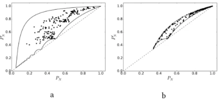
Figure 1: Plots of the minimum and maximum values ofP_N0 as functions ofPNfor (a)N=20and (b)N=5

Figure 1 shows plots of the allowed values ofP0

N (the shaded

area) forN =3 andN=20. Note that only the regionPN ≥1/Nis plotted – sinceWN is the largest weight,PN <1/Nis impossible. Clearly, whenNis relatively large, it is possible forP0

Nto approach

unity even whenPN is small. The effect of I-Roulette appears to be

that when selecting from a large number of edges (as is the case early in the construction of a tour), the highest weighted edge is chosen with disproportionately high probability with respect to the weights.

It is instructive to look at real instances of I-Roulette extracted from runs of an ACO code. Figure 2 shows data extracted from runs of the MMAS algorithm on the d198 TSP test problem. The plots show probabilites derived from weights extracted from cases when ants were choosing between 20 and 3 non-zero weighted edges respectively. The maximum and minimum values ofP0

Nas a

function ofPN, and the lineP_N0 =PNare shown for guidance.

For the caseN =3, I-Roulette selects using probabilities that do not deviate greatly from Roulette Wheel. ForN =20, however, we see that in many cases the algorithmconsiderably amplifies the probability of the most likely edge. These are cases where the selection method is presented with a set of edges in which one edge carries a significantly larger weight than the others. In these cases, the algorithm tends towardsgreedyselection (in which the highest weighted edge is always selected). This situation is more likely to occur at relatively early stages of tour construction , when most of the edges in the nearest-neighbor list are available.

Clearly, I-Roulette is behaving in aqualitatively different way to roulette selection, often amplifying the probability of an edge by a large factor in cases where there are a large number of edges to be chosen from and when one edge carries the majority of the weighting. When there are relatively few edges to choose from, as will occur in the later stages of tour construction, the behavior more closely approximates the proportional probabilities obtained from Roulette Wheel selection.

The effect of I-Roulette in amplifying certain probabilities by large factors may seem counter-intuitive, but the underlying mech-anism is easily demonstrated by example. Consider the case which is schematically represented in Figure 3, in which there are 20 weights, the largest weight is 1, and the other weights are all ap-proximately equal but<0.8. Using Roulette Wheel selection, all the

a b

Figure 2: Values ofP_N0 vs. PN extracted runs of the MMAS algorithm with I-Roulette on the test problem d198 when se-lecting between (a) 20 edges and (b) 3 edges. Data is extracted at the tenth iteration of the algorithm.

Figure 3: Schematic representation of an illustrative prob-lem with 20 weights. See text for details.

choices would carry a probability∼0.05, with slightly higher prob-ability for the highest weighted choice. However, using I-Roulette, we see that there is a probability of 0.2 thatW20is multiplied by a

random number (R₂₀) which is greater than 0.8. In this case, it is impossible for any of the other choices to ‘win’ the process, so the probability of selecting the highest weighted choice is at least 0.2. There will be a small additional contribution from the possibility ofW₂₀R₂₀winning the process whenR₂₀ <0.8, but this will be again∼0.05. Thus, the probability is amplified by a factor of at least four. The I-Roulette probability is dominated in this case by the relative amount by whichW₂₀is greater than its nearest rival, W19. This effect is greater whenNis large, since the roulette wheel

probability varies as 1/N, whereas the I-Roulette probabilityP0

N

is dominated by the relative difference betweenWN andWN−₁,

GECCO ’17, July 15–19, 2017, Berlin, Germany &

Table 1: TSPLIB Instances used for the experimental runs.

Group A

kroA100, kroB100, kroC100, kroD100, kroE100, rd100, eil101, lin105, pr107, pr124, bier127, ch130, pr136, gr137, pr144, ch150, kroA150, kroB150, pr152, u159, rat195, d198, kroA200, kroB200, gr202, ts225, tsp225, pr226, gr229, gil262, pr264, a280, pr299, lin318, rd400, fl417, gr431, pr439, pcb442, d493

Group B att532, ali535, u574, rat575, p654,_{d657, gr666, u724, rat783}

Group C dsj1000, pr1002, u1060, vm1084, pcb1173, d1291, rl1304, rl1323, nrw1379, fl1400, u1432, fl1577, d1655, vm1748, u1817, rl1889

5

EXPERIMENTAL RESULTS

In this section we describe a series of experiments conducted to investigate the effect of I-Roulette on solution quality and conver-gence speed with two ACO variants, using a set of standard test problems.

5.1

Experimental Setup

Runs were carried out using the standard ACOTSP code [17], with a modification to allow the roulette selection procedure to be replaced by I-Roulette. Other than this change, the code is unmodified.

5.1.1 Problem Instance Set. Problem instances were selected

from the TSPLIB [16] library of TSP instances. All instances with 100–2000 vertices and edge weight types supported by ACOTSP were used in the experiments: this gives a total of 65 instances, which are listed in Table 1. For the selection of ACO parameters, these were divided into three groups: those with 100–499, 500–999 and 1000–2000 vertices respectively. For each instance, we ran 50 trials each of ACS and MMAS, both with and without I-Roulette.

5.1.2 Algorithms and Parameters.Runs were carried out using

two ACO variants: Ant Colony System (ACS) and Max-Min Ant System (MMAS). These two variants are among the best perform-ing ACO algorithms for the symmetric TSP. The parameters were chosen based on recommendations in [19], and are listed in Table 2. Note that [19] recommends a small number of ants (m=10) for ACS, and, although their default setting for MMAS ism=nants (wherenis the number of vertices), they obtain better results with fewer ants. Here, we usem =50 for the smaller problems, and m=100 in the larger problems. The runs are limited to a fixed number of tour evaluations: this parameter is set to a different value for each of the three size groups in order to ensure well-converged solutions in all cases. The tour evaluation limit is the same for both MMAS and ACS; since the ACS runs use fewer ants, they run for more iterations, but the total runtime is comparable.

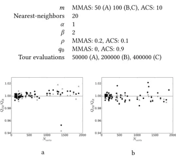
Table 2: ACOTSP parameters for the experimental runs

m MMAS: 50 (A) 100 (B,C), ACS: 10 Nearest-neighbors 20

α 1

β 2

ρ MMAS: 0.2, ACS: 0.1 q₀ MMAS: 0, ACS: 0.9

Tour evaluations 50000 (A), 200000 (B), 400000 (C)

a b

Figure 4: Plots of solution quality ratio (I-Roulette/Roulette) vs. number of vertices for (a) MMAS and (b) ACS. Circles represent mean solutions, crosses best solutions.

5.2

Solution Quality

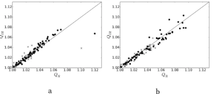
We define thesolution quality,Q, as the ratio of the length of the shortest tourfound in a run to theknown optimumfor the problem instance. The results are summarized in Figure 4, in which we plot the mean values of the solution quality obtained using I-Roulette (QI R) versus those obtained using Roulette Wheel selection (QR)

for ACS and MMAS. Both algorithms obtain very similar solution quality, and the data is clustered closely around the lineQI R =QR.

With MMAS, the solution quality appears to be slightly degraded by using I-Roulette, whereas there is no noticeable effect in the ACS runs. In order to investigate any dependency on the number of vertices, we plot the ratioQI R/QRas a function of number of

vertices in figure 5. Table 3 gives the mean and standard deviation of the ratioQI R/Q_Rfor each group in instances for MMAS and ACS. Values are given for ratios calculated using both the mean and best values ofQ.

Figure 5 (a) shows that MMAS has marginally worse performance with I-Roulette for instances with>1000 vertices, apart from one outlier (instance fl1400), in which I-Roulette appears to perform much better. If this point is discounted, the mean ratioQI R/Q_Rfor MMAS in Group C is 1.0058±0.0022 for mean values, and 1.0048± 0.0060 for best values, which is less than a 0.5% degradation. We conclude, therefore, that I-Roulette does not lead to any significant degradation of the quality of solutions obtained using ACS and MMAS. This conclusion is supported by the data in Table 4, which shows the results of applying the Wilcoxon signed rank test to the paired values of mean and best solution quality. The null hypothesis that the median difference in quality is zero can be rejected for the mean solution quality (hQi) using MMAS, and in this case the size of the effect (from the median difference) is small (0.015).

a b

Figure 5: Plots of solution quality, IRoulette vs. Roulette for (a) MMAS and (b) ACS. Circles represent mean solutions, crosses best solutions.

Table 3: Mean and standard deviation ofQI R/Q_Rfrom the experimental runs. MeanQ BestQ hQ_{I R}/Q_Ri σ(Q_{I R}/Q_R) hQ_{I R}/Q_Ri σ(Q_{I R}/Q_R) A 1.0001 0.0028 1.0003 0.0028 MMAS B 1.0013 0.0033 0.9993 0.0028 C 1.0025 0.0129 1.0010 0.0159 A 0.9996 0.0047 0.9997 0.0031 ACS B 0.9997 0.0043 0.9984 0.0036 C 0.9995 0.0095 0.9980 0.0051

Table 4: Results of statistical tests. ∆is the median differ-ence (I-Roulette minus Roulette) for the quantityx, andpis

the two-sidedp-value from the Wilcoxon signed rank test.

Statistically significantpvalues are in bold face.

x ∆ p hQi 0.015 0.004 MMAS Q_best 0.0003 0.094 T0.05 −3700 0.000 T₀.1 −2400 0.000 hQi −0.005 0.094 ACS Q_best 0.0 0.113 T0.05 −1800 0.000 T₀.1 −480 0.000

5.3

Convergence Speed

We define the quantityTf as the number of tour evaluations in

a run before the solution quality is within a factor 1+f of the best solution found in the run. For example,T0.05is the number

of tours constructed in the run when the solution is within 5% of the best value found at the end of the run. For each problem instance and algorithm, we compute the median over 50 trials of T₀.05andT0.1. These quantities are plotted for the 65 instances in

Figure 6. In all cases, bar one outlier in the MMAS runs, I-Roulette showsconsiderably quicker convergenceto the region of the best solution. The values for all runs are considerably lower than the maximum number of tour evaluations for the experiments, which

a b

Figure 6: Scatter plots of median values for (a)T0.05and (b)

T0.1for IRoulette (y-axis) vs. Roulette (x-axis).

confirms that the solutions obtained are all well converged. As may be expected from the plots, the statistical tests (Table 4) give very strong support to the conclusion that I-Roulette accelerates the convergence to a solution.

6

CONCLUSION AND FURTHER WORK

This paper presents a detailed analysis of I-Roulette, a replacement for Roulette Wheel selection in parallel Ant Colony Optimization. The theoretical analysis shows that the probabilities are modified in a way that tends towards greedy selection in cases where there are a large number of non-zero weights, but reverts to proportional probabilities when faced with fewer choices. The algorithm will therefore tend to greedy selection early in the construction of a tour, but will become more conservative in the later stages. Our experimental results with the MMAS and ACS variants of ACO show that there is no significant effect on solution quality, and that convergence to a solution is greatly accelerated by using I-Roulette. As well as allowing efficient parallel implementations of ACO on hardware such as GPUs, I-Roulette may also confer considerable benefits, by reducing the number of trials required to reach a given quality of solution, accelerating the computation even further.

The results pose a number of questions, which we hope to ad-dress in future work. Firstly, although the behavior of I-Roulette in modifying the probabilities has been determined analytically, and the effects on the solutions obtained have been observed empiri-cally, there is no clear mechanism which links the two:whythe modified probabilities lead to faster convergence remains an open question. An understanding of this mechanism may lead to new variants of the ACO algorithm which use the behavior to improve performance.

Secondly, we have conducted experiments which have shown that there is, on average, little effect on solution quality and, in general, an improvement in convergence speed, but there is con-siderable variation among the problem instances studied here. It may be possible to predict, for a given problem instance, whether I-Roulette may be preferred over Roulette wheel selection orvice versa. Recent work on analyzing the performance of TSP algorithms in terms of problem instance features ([14], [15]) has determined a range of metrics which can predict the performance of some algo-rithms on a given TSP instance. This has enabled the development of techniques for generating instances which are ‘hard’ and ‘easy’.

GECCO ’17, July 15–19, 2017, Berlin, Germany &

A similar analysis could be used to investigate the performance of I-Roulette in ACO.

Finally, this study used fixed values of the algorithm parame-ters. It is possible that a parameter tuning approach could lead to I-Roulette being even more effective in ACO, and the optimum pa-rameters when using I-Roulette may differ from those for Roulette Wheel selection. This is an area for future study.

REFERENCES

[1] Jos´e M. Cecilia, Jos´e M. Garc´ıa, Andy Nisbet, Martyn Amos, and Manuel Ujald´on. 2013. Enhancing Data Parallelism for Ant Colony Optimization on GPUs.J. Parallel Distrib. Comput.73, 1 (2013), 42–51.

[2] J. M. Cecilia, J. M. Garcia, M. Ujaldon, A. Nisbet, and M. Amos. 2011. Paralleliza-tion strategies for ant colony optimisaParalleliza-tion on GPUs. InParallel and Distributed Processing Workshops and Phd Forum (IPDPSW), 2011 IEEE International Sympo-sium on. 339–346. DOI:http://dx.doi.org/10.1109/IPDPS.2011.170

[3] Laurence Dawson. 2015.Generic Techniques in General Purpose GPU Program-ming with Applications to Ant Colony and Image Processing Algorithms. Ph.D. Dissertation. Durham University, UK.

[4] Laurence Dawson and Iain Stewart. 2013. Improving Ant Colony Optimization performance on the GPU using CUDA. In2013 IEEE Conference on Evolutionary Computation, Luis Gerardo de la Fraga (Ed.), Vol. 1. Cancun, Mexico, 1901–1908. [5] Laurence Dawson and Iain A. Stewart. 2013. Candidate Set Parallelization

Strate-gies for Ant Colony Optimization on the GPU. InAlgorithms and Architectures for Parallel Processing: 13th International Conference, ICA3PP 2013, Vietri sul Mare, Italy, December 18-20, 2013, Proceedings, Part I, Joanna Ko lodziej, Beniamino Di Martino, Domenico Talia, and Kaiqi Xiong (Eds.). Springer International Publishing, 216–225.DOI:http://dx.doi.org/10.1007/978-3-319-03859-9 18 [6] Laurence Dawson and Iain A Stewart. 2014. Accelerating ant colony

optimization-based edge detection on the GPU using CUDA. In2014 IEEE Congress on Evolu-tionary Computation (CEC). IEEE, 1736–1743.

[7] Youcef Djenouri, Ahcene Bendjoudi, Malika Mehdi, Nadia Nouali-Taboudjemat, and Zineb Habbas. 2015. GPU-based bees swarm optimization for association rules mining.The Journal of Supercomputing71, 4 (2015), 1318–1344. [8] Marco Dorigo. 1992. Optimization, Learning and Natural Algorithms. Ph.D.

Dissertation. Politecnico di Milano, Italy.

[9] M. Dorigo and L. M. Gambardella. 1997. Ant colony system: a cooperative learning approach to the Traveling Salesman Problem. IEEE Transactions on Evolutionary Computation1, 1 (Apr 1997), 53–66.DOI:http://dx.doi.org/10.1109/ 4235.585892

[10] Marco Dorigo and Thomas St¨utzle. 2004.Ant Colony Optimization. Bradford Company, Scituate, MA, USA.

[11] Jie Fu, Lin Lei, and Guohua Zhou. 2010. A parallel Ant Colony Optimization algorithm with GPU-acceleration based on All-In-Roulette selection. InAdvanced Computational Intelligence (IWACI), 2010 Third International Workshop on. 260– 264.

[12] M. Garland, S. Le Grand, J. Nickolls, J. Anderson, J. Hardwick, S. Morton, E. Phillips, Yao Zhang, and V. Volkov. 2008. Parallel Computing Experiences with CUDA.Micro, IEEE(2008).

[13] Adam Lipowski and Dorota Lipowska. 2012. Roulette-wheel selection via sto-chastic acceptance.Physica A: Statistical Mechanics and its Applications391, 6 (2012), 2193 – 2196.

[14] Olaf Mersmann, Bernd Bischl, Heike Trautmann, Markus Wagner, Jakob Bossek, and Frank Neumann. 2013. A novel feature-based approach to characterize algorithm performance for the Traveling Salesperson Problem.Annals of Mathe-matics and Artificial Intelligence69, 2 (2013), 151–182.DOI:http://dx.doi.org/10. 1007/s10472-013-9341-2

[15] Samadhi Nallaperuma, Markus Wagner, and Frank Neumann. 2015. Analyzing the Effects of Instance Features and Algorithm Parameters for Max-Min Ant System and the Traveling Salesperson Problem.Frontiers in Robotics and AI2 (2015), 18.DOI:http://dx.doi.org/10.3389/frobt.2015.00018

[16] Gerhard Reinelt. 1991. TSPLIB – A Traveling Salesman Problem Library.ORSA Journal on Computing3, 4 (1991), 376–384.

[17] Thomas St¨utzle. 2004. ACOTSP, Version 1.03. http://www.aco-metaheuristic.org/aco-code. (2004). Accessed: 2017-01-31.

[18] T. Stutzle and H. Hoos. 1997. MAX-MIN Ant System and local search for the Trav-eling Salesman Problem. InEvolutionary Computation, 1997., IEEE International Conference on. 309–314.DOI:http://dx.doi.org/10.1109/ICEC.1997.592327 [19] Thomas St¨utzle, Manuel L´opez-Ib´a˜nez, Paola Pellegrini, Michael Maur, Marco

Montes de Oca, Mauro Birattari, and Marco Dorigo. 2012.Parameter Adaptation in Ant Colony Optimization. Springer Berlin Heidelberg, Berlin, Heidelberg, 191–215. DOI:http://dx.doi.org/10.1007/978-3-642-21434-9 8

[20] A. Uchida, Y. Ito, and K. Nakano. 2012. An Efficient GPU Implementation of Ant Colony Optimization for the Traveling Salesman Problem. InNetworking and