SEQUENTIAL RESOURCE ALLOCATION UNDER
UNCERTAINTY: AN INDEX POLICY APPROACH
A Dissertation
Presented to the Faculty of the Graduate School of Cornell University
in Partial Fulfillment of the Requirements for the Degree of Doctor of Philosophy
by Weici Hu August 2017
c
2017 Weici Hu ALL RIGHTS RESERVED
SEQUENTIAL RESOURCE ALLOCATION UNDER UNCERTAINTY: AN INDEX POLICY APPROACH
Weici Hu, Ph.D. Cornell University 2017
We consider a class of stochastic sequential allocation problems - restless multi-armed bandits (RMAB) with a finite horizon and multiple pulls per period. Leveraging the La-grangian relaxation of the problem, we propose an index-based policy that uses the opti-mal Lagrange multipliers to index individual arms, and prove that the policy is asymptot-ically optimal as the number of arms tends to infinity. We also demonstrate numerasymptot-ically that this index-based policy outperforms state-of-the-art heuristics in several instances of RMAB. In addition, we study two other applications of sequential resource allocation problems which are extensions of the RMAB problem, and demonstrate how our index policy can be adapted to these settings.
BIOGRAPHICAL SKETCH
Born as a mainlander, Weici Hu spent most of her childhood in a southern city of China. She then went further south to Singapore to complete her secondary school and high school education. Tired of the tropical climate, she spent the past 8 years acquiring a college degree and trying to acquire a PhD degree in the Northeast of the United States.
ACKNOWLEDGEMENTS
I would like to first thank my advisor for his guidance and extreme patience and for not kicking me out of the program. I would also like to thank my parents for their non-interference policy which has allowed me to experience life in its truest states. Lastly I would like to thank two of my best pals in graduate school: Wei Qian and Kenneth Chong, for handing me water and energy bars during my Marathon race.
TABLE OF CONTENTS
Biographical Sketch . . . iii
Dedication . . . iv
Acknowledgements . . . v
Table of Contents . . . vi
List of Tables . . . viii
List of Figures . . . ix
1 Introduction 1 2 An Asymptotically optimal Index policy for RMAB 7 2.1 Problem Description and Notation . . . 7
2.2 Lagrangian Relaxation and Upper Bounds . . . 9
2.3 An Index Based Heuristic Policy . . . 11
2.3.1 Pre-computations . . . 11
2.3.2 Index policy . . . 14
2.4 Proof of Asymptotic Optimality . . . 15
2.5 Numerical Experiments . . . 24
2.5.1 Multi-armed bandit . . . 24
2.5.2 Project assignment problem . . . 26
2.5.3 Subset selection problem . . . 27
2.6 Conclusion . . . 29
3 Parallel Bayesian Policies For Finite Multiple Comparisons With a Known Standard 30 3.1 Introduction . . . 30 3.2 Problem Formulation . . . 34 3.3 Upper Bound . . . 38 3.4 Index Policy . . . 44 3.5 Numerical Results . . . 47 3.6 Conclusion . . . 49
4 Bayes-Optimal Effort Allocation in Crowdsourcing: Bounds and Index Policies 50 4.1 Introduction . . . 50
4.2 Related Work . . . 53
4.3 Problem Statement . . . 54
4.4 Dynamic Programming Formulation . . . 56
4.5 Upper Bound on the Bayes-Optimal Policy . . . 61
4.6 Index Policy . . . 67
4.7 Numerical Experiment . . . 68
4.7.1 Simulation using simulated data . . . 68
4.7.2 Simulation using real data . . . 71
A 73
A.1 Notation of Chapter 2 . . . 73
A.2 Upper Bound . . . 75
A.3 Decomposition . . . 76
A.4 Show arg infλλλ∈RTP(λλλ) is non-empty . . . 76
A.5 Proof of the existence ofπ∗∗ . . . 77
A.6 Proof ofT∗maxs,a,trt(s,a) upper boundsβt(s) . . . 78
A.7 A result that justifies using bisection . . . 79
A.8 Proof of Lemma 3 . . . 79
A.9 Proof of Lemma 4 . . . 80
A.10 Lemma 14 . . . 81
A.11 Proof of Lemma 5 . . . 82
A.12 Proof of Lemma 6 . . . 84
A.13 Proof of Lemma 7 . . . 85
A.14 Bellman’s recursion forT =∞ . . . 87
LIST OF TABLES
LIST OF FIGURES
2.1 Upper bound and simulation results of MAB . . . 25 2.2 Upper bound and simulation result of project assignment problem . . . 27 2.3 Upper bound and simulation result of subset selection . . . 29 3.1 This figure illustrates howzn is chosen by the index-based policy with
k = 2 systems, m = 2 parallel computing resources, andN = 20 sim-ulation batches. Figure (a) plots zλλλ2,2, the optimal number of samples to take in batch 3 from system 1 when it is in state (2,2), against the value ofλ; Figure (b) plotszλλλ3,3, the optimal number of samples to take in batch 3 from system 2 when it is in state (3,3). Figure (c) plots
zλλλ2,2+zλλλ3,3, the optimal total number of samples to take across both sys-tems. The dashed line in (c) shows the constraint m = 2, and λ∗ will
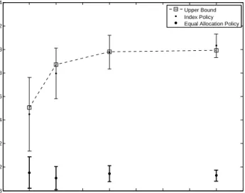
be the left endpoint of the solid line overlapping this dashed line. The number of samples taken from each system will bezλλλ2∗,2 =1 andzλλλ3,∗3 = 1 respectively. . . 46 3.2 This figure shows the upper bound on the performance of the optimal
policy for the MCS problem (dashed line with squares) normalized by dividing byk, as well as the estimated performance of two sub-optimal policies: the index policy from Section 4.6 (thinner lines and dots); and the equal allocation policy (thicker lines and dots). The setting pictured usesm=k,dx =0.2,α0x = β0x = 1,cx =0. We use 10,000 independent replications to estimate the value of the index policy, and 50,000 for the equal allocation policy. The plot shows that the index policy is substan-tially better than equal allocation, and is statistically indistinguishable from optimal given the number of replications performed. . . 48
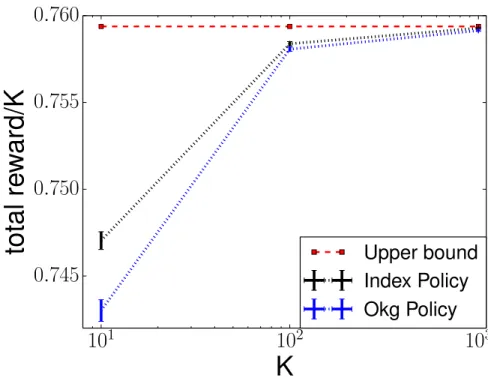
4.1 Semi-log plot ofKagainst average per task reward (R/K) forK =10,102,103. 69
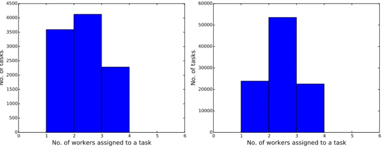
4.2 Histogram of number of workers assigned to a task . . . 70
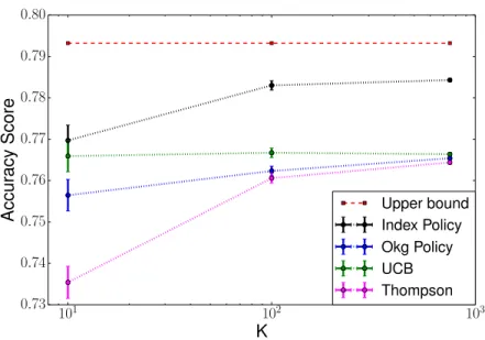
4.3 Semi-log plot ofKagainst accuracy score forK=10,100,750. . . 72
CHAPTER 1
INTRODUCTION
We consider a general class of dynamic resource allocation problems with average-case criteria. Such problems enjoy a variety of applications in a wide range of industries. Examples include:
• Facebook displays ads in thesuggested postssection every time its users browse their personal pages. Among the ads that have been shown, some are known to attract more clicks than others. But there are also many ads which have yet to be shown and they may attract even more clicks. Given that the slots for display are limited, a policy is required to select ads to maximize total clicks.
• In a multi-stage clinical trial, a medical group starts with a number of new treat-ments and an existing treatment with reliable performance. In each stage, a few treatments are selected from the pool to test, with the goal to identifying the new treatments that perform better than the existing one with high confidence. A strat-egy is required to select which treatments to test at every stage to most effectively support their judgment at the end of the trial.
• A data analyst wishes to label a large number of images using crowdsourced effort from low-cost but potentially inaccurate workers. Each label given by the crowd-workers comes with a cost and the analyst has limited budget. Hence she needs to carefully assign tasks to workers so as to maximize the likelihood of correct labeling.
We formulate such problems as instances of the restless multiarmed bandit (RMAB) problem [48] with a finite horizon and multiple pulls per period, which, in turn, is closely related to a broader class of problem calledWeakly Coupled Dynamic Programs
(WCDP) [25]. In the RMAB, we have a collection of “arms”, each of which is endowed with a state that evolves independently. If the arm is “pulled” or “engaged’ in a time period then it advances stochastically according to one transition kernel, and if not then it advances according to a different kernel. Rewards are generated with each transition, and our goal is to maximize the expected total reward over a finite horizon, subject to a constraint on the number of arms pulled in each time period. The RMAB forms a generalization of the more famous multi-armed bandit (MAB) [41] by allowing arms that are not engaged to change state and multiple pulls per period.
Theoretically an optimal solution of a RMAB can be obtained by leveraging the Bell-man equationand solving it as a dynamic program (DP) [40]. However, this approach becomes computationally infeasible when the state space grows large. In particular, the state space grows exponentially with the number of arms in a RMAB, and the number of arms are often large in practice. This approach therefore suffers the so-called “curse of dimensionality” [39]. Much research has been dedicated to efficiently finding “good” solutions. Gittin in 1979 proposed a tractable-to-compute optimal policy for the infinite horizon MAB with one pull per time period, which is famously known as the Gittins index policy [21]. This policy is appealing because it can be computed by considering the state space for only a single arm, making it computationally tractable for problems with many arms. This policy loses its optimality properties, however, when modifying the problem in any problem dimension: when allowing arms that are not engaged to change state; when moving to a finite horizon [6]; or when allowing multiple pulls per period. Thus, the Gittins index does not apply to our problem setting.
While the RMAB is not known to have a computable optimal policy, [48] proposed a heuristic called the Whittle index for the infinite-horizon RMAB with multiple pulls per period, which is well-defined when arms satisfy an indexability condition. This policy
is derived by considering a Lagrangian relaxtion of the RMAB in which the constraint on the number of arms pulled is replaced by a penalty paid for pulling an arm. An arm’s Whittle index is then the penalty that makes a rational player indifferent between pulling and not pulling that arm. The Whittle index policy then pulls those arms with the highest Whittle indices. Appealingly, the Whittle index and the Gittins index are identical when applied to the MAB problem with a single pull per period. [48] further conjectured that if the number of arms and the number of pulls in each time period go to infinity at the same rate in an infinite-horizon RMAB, then the Whittle index policy is asymptotically optimal when arms are indexable. [46, 47] gave a proof to Whittle’s conjecture with a difficult-to-verify condition: that the fluid approximation has a globally asymptotically stable equilibrium point. This condition was shown to hold when each arm’s state space has at most 3 states, but this condition does not hold in general and [46] provides a counterexample with 4 states.
Our contribution in this dissertation is to (1) create an index policy for finite horizon RMABs with multiple pulls per period, and (2) show that it is asymptotically optimal in the same limit considered by Whittle. Like the Whittle index, our approach is com-putationally appealing because it requires considering the state space for only a single arm, and its computational complexity does not grow with the number of arms. Un-like the Whitle index, our index policy does not require an indexability condition to be well-defined, and in contrast with [46, 47] our proof of asymptotic optimality holds re-gardless of the number of states, and does not depend on hard-to-verify conditions. We further demonstrate our index policy numerically on problems from the literature that can be formulated as finite-horizon RMABs, and show that it provides finite-sample performance that improves over the state-of-the-art. We also use our framework to de-velop policies for two major RMAB-like applied problems: Multiple comparison with a standard (MCS) in the field of simulation and crowdsourcing in the field of artificial
intelligence, and demonstrate numerically that our index-based policies out-perform the state-of-art using both real and synthetic data.
In addition to building on [48, 46, 47], our work builds on the literature in weakly coupled dynamic programs (WCDP), that itself builds on RMABs. Indeed, at the end of his paper, Whittle pointed out that his relaxation technique can be applied to a more gen-eral class of problems in which sub-problems are linked by constraints on actions, but are otherwise independent. Hawkins in his thesis [25] formally termed these problems (but with a more general type of constraints) as WCDPs and proposed a general decou-pling technique. Moreover, he proposed a minimal-lambda policy for infinite horizon WCDPs which, like the Whittle index policy, is derived by considering a Lagrangian relaxation of the WCDP. The minimal-lambda policy finds the smallest Lagrange mul-tiplier so that the current optimal decision for the Lagrangian relaxation is also feasible for the original WCDP. The minimal-lambda policy then pulls arms according to this optimal decision. In the case of RMAB, the minimal-lambda policy is equivalent to the Whittle index with the smallest of the indices of all pulled arms for the former being the same as the smallest Lagrange multiplier to attain a feasible solution for the latter.
Another major work in WCDP is [1] which shows that the ADP relaxation is tighter than the Lagrangian relaxation but is also computationally more expensive. It gives necessary and sufficient conditions for the Lagrangian relaxation to be tight and proves that the optimality gap is bounded by a constant when the Lagrange multipliers are allowed to be state dependent. The last result that the optimality gap is bounded by a constant implies that the per arm gap goes to zero as the number of arms grows. We achieve a similar result in the dissertation by showing the per arm reward of our index-based heuristic policy goes to the per-arm reward of the Lagrangian bound, despite that our Lagrange multipliers not being state-dependent. While there are similarities between
the two works, the focus differs: while our work focuses on offering an asymptotically optimal heuristic policy, [1] examines the ordering and tightness of different bounds. The heuristic proposed in [1] is based on an ADP technique, and is different from our index-based policy.
Other work on WCDP also includes [52] who proposes an even tighter bound by incorporating an information relaxation on the non-anticipative constraints in addition to the existing relaxation methods. [24] considers two classes of large-scale WCDPs in which the state and action space in each sub-problem also grows exponentially and uses an ADP technique to approximate the value functions of individual sub-MDPs in addition to employing a Lagrangian relaxation for the overall problem.
In this thesis, we use Chapter 2 to present the main theoretical work on RMAB and propose an index-based policy. Chapter 3 and 4 present applied problems that are similar to RMAB but with some variations, and index-based policies for these problems. Below is a brief outline of the chapters in the dissertation:
• In Chapter 2, we consider the RMAB with a finite horizon and multiple pulls per period. Leveraging a Lagrangian relaxation, we approximate the RMAB with a problem that can be decomposed into a collection of single arm problems. We then propose an index-based policy that uses optimal solutions of the single arm problems to index individual arms, and offer a proof that it is asymptotically op-timal as the number of arms tends to infinity. We also use simulation to show that this index-based policy performs better than the state-of-art heuristics in various problem settings.
• In Chapter 3, we consider the problem of multiple comparisons with a known stan-dard, in which we wish to allocate simulation effort efficiently across a finite num-ber of simulated systems, to determine which systems have mean performance
exceeding a known threshold. We suppose that parallel computing resources are available, and that we are given a fixed simulation budget. We consider this prob-lem in a Bayesian setting, and formulate it as a stochastic dynamic program. The set-up of the problem is the same as a RMAB except that every simulated sys-tem (the arms) is allowed to have multiple computing resources (the pulls) in a time period. For simplicity, we focus on Bernoulli sampling, with a linear loss function. Using links to restless multi-armed bandits, we provide a computation-ally tractable upper bound on the value of the Bayes-optimal policy, and an index policy motivated by these upper bounds. This chapter has been published in the proceedings of the 2014Winter Simulation Conference.
• In Chapter 4, we consider effort allocation in crowdsourcing, where we wish to as-sign labeling tasks to imperfect homogeneous crowd workers to maximize overall accuracy in a continuous-time Bayesian setting, subject to budget and time con-straints. The Bayes-optimal policy for this problem is the solution to a partially observable Markov decision process, but the curse of dimensionality renders the computation infeasible. Based on the Lagrangian Relaxation technique in [1], we provide a computationally tractable instance-specific upper bound on the value of this Bayes-optimal policy, which can in turn be used to bound the optimality gap of any other sub-optimal policy. In an approach similar in spirit to the Whittle index for restless multi-armed bandits, we provide an index policy for effort allo-cation in crowdsourcing and demonstrate numerically that it outperforms the state of the art and is near-optimal. This chapter has been published in the proceedings of the 2016Artificial Intelligence and Statistics Conference.
CHAPTER 2
AN ASYMPTOTICALLY OPTIMAL INDEX POLICY FOR RMAB
Chapter 2 presents the major theoretical work of this dissertation. In this chapter, Section 2.1 formulates the problem, Section 2.2 discusses the Lagrangian relaxation of the problem, Section 2.3 states our index-based policy and provides computational methods, Section 2.4 gives a proof of asymptotic optimality, Section 2.5 numerically evaluates our index policy, and Section 7 concludes.
2.1
Problem Description and Notation
We consider an MDP (SK,AK,P,R) which is created by a collection ofK sub-processes
(S,A,P,r). The sub-processes are independent of each other except that the actions
taken by each sub-process have to jointly satisfy some constraints at each time step. These sub-processes are also referred to as arms in the bandit literature and shall be indexed by x ∈ {1, ...,K}. Following a standard construction for MDPs, both the larger joint MDP and the sub-processes will be constructed on the same measurable space (Ω,F). Random variables on this measurable space will correspond to states, actions, rewards, and each policy will induce a probability measure over this space.
We describe the MDP to consider formally as comprising:
• Thetime horizonT <∞.
• Thestate space SK is the cross product ofKsub-processes’ state spaceS, which
is assumed to be finite. We uses = (s1, ...,sK) to denote an element inSK andS
when the state is random. We also useSt to emphasize that the state is at timet. Likewise, we usesto denote an element inS, andS orSt when it is random.
• Theaction spaceAK is the cross product of K sub-processes’ action spaceA = {0,1}. We usea to denote a generic element ofA, and Awhen it is random. We usea=(a1,a2, ...,aK) to denote a generic element inAKandAwhen it is random.
In the context of bandit problems,a=1 is called “pulling” an arm (sub-process). • The reward function Rt : SK × AK 7→ R for each 1 ≤ t ≤ T. Rt(s,a) =
PK
x=1rt(sx,ax), wherert(sx,ax) is the reward obtained by a sub-process when ac-tion ax is taken in state sx at time t. We assume rewards are non-negative and finite.
• Thetransition kernelPa(s0,s) =QK x=1P
ax(s0
x,sx), whereP
a(s0,s) is the
probabil-ity of a sub-process transitioning from s0 to sif action ais taken, i.e., P(s|s0,a).
The product implies that theKsub-processes evolve independently. RMAB differ from MAB in that MABs requireP0(s,s)= 1 while RMABs allows P0(s,s) < 1.
Since we are considering both cases, we do not restrict the value ofP0(s,s).
Next we describe the set of policies for our MDP problem. Since the state and action space defined above are finite, it is sufficient to consider the set of Markov policies Π [40]. Define a policy πππ ∈ Π as a function SK × AK × {1, ...,T} → [0,1]
that determines the probability of choosing action a in state s at time t. Subse-quently we have P
a∈AKπππ(s,a,t) = 1, ∀s ∈ S K,∀
1 ≤ t ≤ T. A policy πππ and the transition kernel P·(·,·) together defines a probability distribution Pπππ on all possible
paths of the process {s1a1...sT : st ∈ SK,at ∈ AK}. Starting at a fixed state s1, i.e.,
Pπππ(S1 = s1) = 1, we have the conditional distributions ofSt andAt defined recursively byPπππ(St+1= s0|St =s,At =a)=Pa(s,s0) and Pπππ(At =a|St =s)=πππ(s,a,t).
The MDP we are considering allows exactlymsub-processes to be set active at each time step. Hence a feasible policy,πππ∈Π, has to satisfyPπππ(|At|=m)=1,∀t∈ {1, ...,T}. Here we use| · |as an operator that sums all the elements in a vector.
The objective of our MDP is: maximize πππ∈Π E πππ T X t=1 Rt St,At subject to Pπππ(|At|=mt)= 1, ∀1≤ t≤T. (2.1)
Since we will discuss other MDPs in the process of solving this one, (2.1) will be re-ferred to as theoriginalMDP in the rest of the chapter to avoid confusion. For conve-nience, we summarize our notation in Appendix A.1.
The original MDP (2.1) suffers from the “curse of dimensionality”, and hence solv-ing it is computationally intractable. In the remainder of the chapter we build a compu-tationally feasible index-based heuristics with a performance guarantee.
2.2
Lagrangian Relaxation and Upper Bounds
In this section we discuss the Lagrangian relaxation of the original MDP and the cor-responding single process problem. These single process problems together with the Lagrange multipliers form the building blocks of our index-based policy, which will be formally introduced in Section 2.3. The Lagrangian relaxation considers an uncon-strained problem whose objective is obtained by augmenting the objective of (2.1):
P(λλλ)=max πππ∈Π E πππ T X t=1 Rt St,At −Eπππ T X t=1 λt(|At| −mt) , (2.2) for anyλλλ={λ1, ..., λT} ∈RT
. This unconstrained problem has the following property:
Lemma 1. For anyλλλ ∈RT, P(λλλ)is an upper bound to the optimal value of the original
MDP.
straightforward proof by viewingP(λλλ) as the Lagrange dual function of a relaxed
prob-lem of the original MDP; see Appendix A.2.
This Lagrangian relaxation then decomposes into K smaller MDPs, which we can easily solve to optimality. To elaborate on this idea of decomposition, we construct a
sub-MDPproblem based on tuple (S,A,P·(·,·),r(·,·)). Again we consider only the set
of Markov policies, Π, for this problem. Similarly a policy π ∈ Π is a function that determines the probability of choosing action a in state s at time t, i.e., π : S× A× {1, ...,T} → [0,1]. The sub-MDP starts at a fixed state s1. Subsequently we can define
distributions ofSt and At under Pπ in a similar manner as we did forSt and At in the previous section. The objective of the sub-MDP is:
Q(λλλ)= max π∈Π E π T X t=1 rt(St,At)−λtAt . (2.3)
We are now ready to present the decomposition of the Lagrangian relaxation.
Lemma 2. The optimal value of the relaxed problem satisfies
P(λλλ)= KQ(λλλ)+X
t
mtλt, (2.4)
[1] also gave a proof to Lemma 2, and we again provide a different proof in Appendix A.3. Since the state space of the sub-MDP is much smaller, we can solve it directly by using backward induction and the optimality equation. The existence of such an optimal Markov deterministic policy follows from that the state and action spaces of the sub-MDP being finite [40]. Let Π∗(λλλ) be the set of optimal Markov deterministic policies of the sub-MDP for a givenλλλ. The relaxed problem can be solved by combining the solutions of individual sub-MDPs, that is, we can construct an optimal policy of the relaxed problemπππλλλ by settingπππλλλ(s,a,t) = QK
x=1πλλλ(sx,ax,t), where πλλλ is an element in
2.3
An Index Based Heuristic Policy
Our index based heuristic policy assigns an index to each sub-process, based upon its state and current time. At each time step, we set active the m sub-processes with the highest indices. Before carrying out the process of sequential decision-making, our index policy calls for pre-computation of 1)λλλ∗∈arg infλλλP(λλλ), as defined in Section 2.2;
2) a set of indices,βββ, that will later be used for decision-making at every time step; 3) an optimal policyπ∗∗ for the sub-MDP problem in (2.3). In the first part of this section
we discuss how we carry out such computations.
2.3.1
Pre-computations
Dual optimalλλλ∗
We use subgradient descent to solve infλλλP(λλλ), which converges to its solutionλλλ∗ by convexity ofλλλ7→ P(λλλ) (Theorem 7.4 in [42]). By (2.3) and (2.4), a sub-gradient ofP(λλλ)
with respect toλλλ is given by (−KEπλλλ[At]+m : 1 ≤ t ≤ T), whereπλλλ is any policy in
Π∗(λλλ).
To compute this sub-gradient, we compute a policy πλλλin Π∗(λλλ) and then use exact
computation or simulation with a large number of replications to computeEπ
λλλ
[At]. To compute a policy inΠ∗(λλλ), we first compute the value functionVλλλ : S× {1, ...,T} 7→ R
of sub-MDPQ(λλλ). We accomplish this using backward induction [40]:
Vλλλ(s,t)= maxa∈A{rT(s,a)−aλT} ift =T, maxa∈A{rt(s,a)−aλt+ P s0∈ SP a(s,s0)Vλλλ(s0,t+1)} otherwise. (2.5)
Recalling that Π∗(λλλ) includes only deterministic policies, a policy πλλλ in Π∗(λλλ) are
rt(s,a)−aλt+P
s0∈ SP
a
(s,s0)Vλλλ(s0,t+1) is equal toVλλλ(s,t), and then settingπλλλ(s,a,t)=1 for thisa. For those sand t for which both actionsa have one-step lookahead values equal toVλλλ(s,t), one may setπλλλ(s,a,t) =1 for either such action. Thus, the cardinality ofΠ∗(λλλ) is 2 raised to the power of the number ofs,tfor which the one-step lookahead
values for playing and not playing are tied.
When we construct a policy inΠ∗(λλλ) for the purpose of computing a sub-gradient of P(λλλ), we choose to play in those s,t with tied one-step lookahead values. While our subgradient descent algorithm would converge for other choices, making this choice better supports computation of indices in section 2.3.1.
Indicesβt(s)
Define the vectorv[a,t] to bev+(a−vt)∗et, that is, the vectorvwith thetthelement replaced bya∈R. We define theindexof states∈Sat timetas
βt(s)= sup{β:∃π∈Π∗(λλλ∗[β,t]) s.t. π(s,1,t)= 1}. (2.6)
Instead of computing the entire set Π∗(λλλ∗[β,t]), we only need to compute a policy in
Π∗(λλλ∗[β,t
]) using the method discussed in section 2.3.1, i.e., always choose the active action when there are ties. Intuitively, this index is the maximum price we are willing to pay to set a sub-process active in state s at t. By leveraging the monotonicity of optimal actions with respect to rewards, as shown in Lemma 13 in Appendix A.7, we compute βt(s) via bisection search in the interval [0,U], where U upper bounds the largest possible value ofβt(s). For example, we can setU asT ∗maxs,a,trt(s,a) when λλλ∗ ≥
0 (we show in Appendix A.6 that βt(s) cannot be greater than this value in this case). We pre-compute the setβββ = {βt(s) : s ∈ S,1 ≤ t ≤ T}before running the actual algorithm.
Occupation measureρ∗and its corresponding optimal policyπ**
Our tie-breaking policy involves constructing an optimal Markov policyπ∗∗for the sub-MDP Q(λλλ∗) such that Eπ∗∗[At] = mK, ∀1 ≤ t ≤ T. The existence of π∗∗ is shown in Appendix A.5. To compute π∗∗, we borrow the idea of the occupation measure [18].
Define the occupation measure,ρ(s,a,t), induced by a policyπto be the probability of being in statesand taking actionaat timetunderπ. Subsequentlyπ∗∗can be computed by solving the following linear program (LP):
max
{ρ(s,a,t):y∈S,a∈A,t∈{1,...,T}}
T X t=1 X a∈A X s∈S ρ(s,a,t)rt(s,a) subject to X s∈S ρ(s,1,t)= mt K,∀t =1. . . . ,T X a∈A ρ(s,a,t)−X a∈A X s0∈ S ρ(s0,a,t−1)Pa(s0,s)=0, ∀s∈S,2≤ t≤T X a∈A ρ(s,a,1)=1(s= s1) ∀s∈S ρ(s,a,t)≥ 0, ∀s∈S,a∈A,t=1, . . . ,T, (2.7)
The first constraint ensures thatEπ
∗∗
[At] = mK. The second constraint ensures flow bal-ance. The third constraint shows that we start at states1. The second and third constraint
together implyP
a∈A,s∈Sρ(s,a,t) = 1, i.e., that (ρ(s,a,t) : a ∈ A,s ∈S) is a probability distribution for each t. The fourth and fifth constraints ensure thatρis a valid probability measure.
Letρ∗be an optimal solution to (2.7). π∗∗ can then be constructed by
π∗∗ (s,a,t)= ρ∗ (s,a,t) P a∈Aρ ∗(s,a,t), if P a∈Aρ ∗ (s,a,t)>0 1(a= 1), if P a∈Aρ ∗(s,a,t)=0 andβt(s)≥ λ∗ t 1(a= 0), if P a∈Aρ ∗(s,a,t)=0 andβt(s)< λ∗ t, (2.8)
for all s∈S,a∈A,1≤ t≤T.
Here we also make an observation thatλλλ∗ ∈arg minP(λλλ∗) is the optimal dual variable
corresponding to the first constraint in 2.7.
2.3.2
Index policy
Let{βt(St,x) : x∈ {1, ...,K}}be the indices associated with the K sub-processes at timet. We define ¯βt(St) to be the largest valueβin{βt(St,x) : x∈ {1, ...,K}}such that at leastm
sub-processes have indices of at leastβ. Our index policy then sets the actions of sub-processes with indices strictly greater than ¯βtto 1 (active), and those with indices strictly less than ¯βt to 0 (inactive). When more thanmsub-processes have indices greater than or equal to ¯βt, a tie-breaking a rule is needed. For simplicity, in the following discussion we use the term remaining resources to refer to the remaining number of the arms to be set active after we activate all the arms with indices greater than ¯βt(St), and use
It = {St,x : 1 ≤ x ≤ K, βt(St,x) = βt(¯ St)} to denote the set of states occupied by the sub-processes with tied indices. Our tie-breaking rule allocates the remaining resources acrossIt according to the probability distribution induced byπ∗∗overSat timet. More specifically, we allocate qt(St,x)= ρ∗(S t,x,1,t) P s0∈Itρ∗(s0,1,t), if P s0∈I tρ ∗ (s0,1,t)>0 Nt(St,x) P s0∈ItNt(s0), otherwise (2.9)
fraction of the remaining resources to each of the state in It, where Nt(s) denote the number of sub-processes in statesat timet.
We then use the function Rounding(total, frac, avail) in Algorithm 2 to deal with situations where the products between the desired fractions and the remaining resources
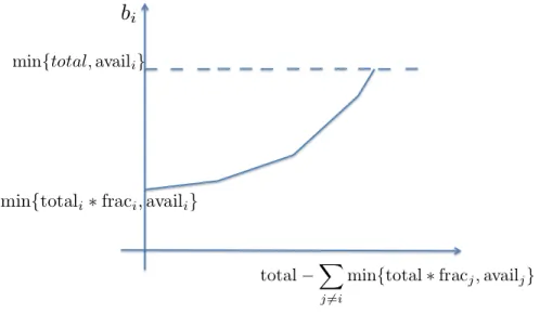
are not integers. Here total represents the number of remaining resources, f rac is a vector of the fractions of the remaining resources to be approximated allocated to each tied state, and availis a vector of the number of sub-processes in each tied state. The function also allows the number of sub-processes in a tied state s to be less than the number of resources we would like to assign to saccording to the fraction in (2.9). We note the following property of this function Rounding, which we will rely on in our proof in Section 6.
Remark 1. When total, avail, frac satisfy availi ≥ total∗fraci, the output vector b =
Rounding(total,frac,avail)satisfies|bi−total∗fraci|< 1for all i.
This tie-breaking ensures asymptotic optimality of the index policy as it enforces that the fraction of sub-processes in each state sis equal to the distribution induced by π∗∗
in the limit. This idea shall become clear in Section 2.4 where the proof of asymptotic optimality is presented.
We formally present our index policy in Algorithms 1 and 2.
2.4
Proof of Asymptotic Optimality
Our index policy ˆπππ achieves asymptotic optimality when we let the number of sub-processes K go to infinity, while holding αt = mt
K constant for all t. Let Z(πππ,m,K) to denote the expected reward of the original MDP obtained by policyπππ with K sub-processes andm = (m1, ...,mT) constraints at each time. We useΠm,K to denote the set
of all feasible Markov policies for the such an MDP. Lastly, it should be understood that whenever we use ˆπππto denote our index policy there is a dependency of ˆπππonm andK
Algorithm 1: Index Policy ˆπππ
Pre-compute:λλλ∗;βββ;ρ∗. (Refer to section 2.3.1 for computational details) fort=1, ...,T do
Let βt,[i] be the ith largest element in the listβt(St,1), ..., βt(St,K), so βt,[1] ≥ . . . ≥
βt,[K].
Let ¯βt =βt,[m]
LetIt = {s:βt(s)=βt¯ ands= St,x for some x} LetNt(s)= |{x:St,x = s}|, for all s.
Fors∈It, let qt(s)= ρ∗(s,1,t) P s0∈Itρ∗(s0,1,t), if P s0∈I tρ ∗ (s0,1,t)> 0 Nt(s) P s0∈ItNt(s0), otherwise Letb=Rounding(m−P s0:β t(s0)>β¯t Nt(s 0),(qt(s) : s∈It),(Nt(s) : s∈It)) forall sdo
Ifβt(s)> βt, set all¯ Nt(s) sub-processes insactive. Ifβt(s)= βt, set¯ b(s) sub-processes in sactive. Ifβt(s)< βt, set 0 sub-processes in¯ sactive.
end for end for
which shows that the per arm gap between the upper bound and the index policy goes to zero under the limit assumption.:
Theorem 1. For anyααα∈(0,1)T,
lim K→∞ 1 K Z( ˆπππ,bαααKc,K)−πππ∈maxΠbαKc,K Z(πππ,bαααKc,K) ! = 0, (2.10) wherebαααKc=(bα1Kc, ...,bαTKc)
Algorithm 2: Rounding(total, frac, avail) Inputs: total (a scalar), frac (a vector satisfying P
ifraci = 1), avail (a vector of the same length as frac satisfying total≤ P
iavaili)
Output:b(a vector of the same length as the inputs satisfyingP
ibi = total,bi ≤availi) Letn=length(frac)
Let bi = min{availi,btotal∗fracic}, fori=1, ...,n. Let j=1 whiletotal>Pn i=1bi do Let bj = bj+1(availj > bj) Let j= (j mod n)+1 end while return b
We first point out that the optimal solutions of maxπππ∈ΠbαKc,KZ(πππ,bαααKc,K) are trivial
whenα=0or1. So we do not include these two cases when we consider convergence of the index policy ˆπππ. To formalize the notations that will be used throughout the proofs, we augmentP(λλλ) toP(λλλ,m,K) to indicate the values ofmandKassumed in the Lagrangian relaxation. We useλλλ∗to denote one and any element in arg infλλλP(K, αααK, λλλ) and letπ∗∗
be the optimal policy constructed in (2.8) usingmt = αtK, which satisfiesEπ
∗∗
(At)= αt for allt. Noteλλλ∗andπ∗∗ depend on onlyααα(not onK).
As before, we let Nt(s) be the number of sub-processes in state sat timetunder ˆπππ. We additionally define Mt(s) to be the number of sub-processes in statesat timetthat are set active by ˆπππ. These quantities depend onK andm, but for simplicity we do not include this dependence in the notation. We always assumem = bαααKcand we rely on context to make clear the value ofKassumed. We also defineVt(s) to be the set of states with the same index value as s, includings, and Ut(s) to be the set of states with index
value greater than that of s, for each timet. These quantities depend onαααbut not onK
orm.
We prove Theorem 1 by first demonstrating below in Theorem 2 that for each time
t, the proportion of the sub-processes that are in state sunder our index policy ˆπππ, Nt(s)
K , approachesPt(s) asK → ∞. In other words, our index policy ˆπππrecreates the behavior ofπ∗∗in the largeK limit.
Theorem 2. For every s∈Sand1≤ t≤T ,
lim K→∞ Nt(s) K = Pt(s), P ˆ πππ−a.s., (2.11) and lim K→∞ Mt(s) K = Pt(s)∗π ∗∗ (s,1,t), Pπππˆ −a.s., (2.12)
Before proving Theorem 2, we first present two intermediate results, whose proofs are given in Appendix A.8 and A.9.
Lemma 3. At time1≤t≤ T , for all s∈S, we have
(1) Ifβt(s)> λ∗ t, thenπ ∗∗(s,1,t)= 1. (2) Ifβt(s)< λ∗t, thenπ ∗∗ (s,1,t)= 0.
Lemma 4. For any state s∈Sand time1≤t≤ T ,
(1) Ifαt−P s0∈U t(s)∪Vt(s)Pt(s 0)≥0, thenπ∗∗(s,1,t)=1. (2) Ifαt−P s0∈U t(s)Pt(s 0 )≤0, thenπ∗∗(s,1,t)=0.
Proof. We prove (2.11) and (2.12) simultaneously via induction over the time periods. Whent =1, all sub-processes starts in state s1, and we have
lim K→∞ N1(s) K = Klim→∞ K K =1= P1(s) ifs= s1, lim K→∞ N1(s) K =Klim→∞ 0 K =0= P1(s) otherwise.
By the set-up of the original MDP,M1(s)= bα∗Kc, and we have
lim K→∞ M1(s) K = Klim→∞ bα∗Kc K = α= π ∗∗ (s,1,t)= P1(s)∗π∗∗(s,1,t), ifs= s1, lim K→∞ M1(s) K = 0 K = 0= P1(s)∗π ∗∗ (s,1,t), otherwise,
so we have proved the base case of the induction.
Now assume (2.11) and (2.12) hold up until time t. Fix a state s ∈ S and time 1≤t≤ T, defineYt(s0,s) to be the number of sub-processes set active by ˆπππin s0at time
twhich transition to state sat timet+1, andXt(s0,s) to be the number of sub-processes set inactive by ˆπππin s0at timetwhich transition tosat timet+1. Note thatYt(s0,s) and
Xt(s0,s) also depend onK. We can subsequently expressN
t+1(s) as Nt+1(s)= X s0∈ S Yt(s0,s)+Xt(s0,s). Dividing both sides byK, and takingK to a limit, we get
lim K→∞ Nt+1(s) K =Klim→∞ X s0∈ S 1 KYt(s 0, s)+ lim K→∞ X s0∈ S 1 KXt(s 0, s). (2.13) Note Yt(s0,s) is a binomial random variable with Mt(s0) trials and success probability
P1(s0,s). Similarly,Xt(s0,s) is a binomial random variable withN
t(s0)−Mt(s0) trials and success probabilityP0(s0,s). We can rewrite the RHS of (2.13) by applying Lemma 14,
which is stated in Appendix A.10: lim K→∞ Nt+1(s) K = X s0∈ S lim K→∞ Mt(s0) K ∗P 1(s0,s ) (2.14) +X s0∈ S lim K→∞ Nt(s0)−Mt(s0) K ∗P 0 x(s 0, s) =X s0∈ S Pt(s 0 )∗π∗∗(s0,1,t+1)∗P1(s0,s) (2.15) +X s0∈ S Pt(s0)(1−π∗∗(s0,1,t+1))∗P0x(s0,s) a.s. = Pt+1(s). a.s. (2.16)
The last equality follows as we have exhausted all the ways of getting tosat timet+1. Hence we have shown (2.11) holds for timet+1.
Next we show (2.12) holds for timet+1. We define setsPt = {Pt(s) : s ∈ S}, and Nt = {Nt(s) : s ∈ S}. RecallVt(s) is the set of states with the same index value as s,
includings, andUt(s) is the set of states with index value greater than that of s, we let
Nt+(s)= P s0∈U t(s)Nt(s 0) andN= t (s)= P s0∈V t(s)Nt(s 0). We use notation Nt
K for the set which consists of all elements inNt divided byK. Lastly we use the function fs(Nt,bαtKc) to represent the number of sub-processes set active at timetin states:
fs(Nt,bαtKc)=
1
([bαtKc−N+t (s)]+≥Nt=(s))∗Nt(s)
+
1
([bαtKc−Nt+(s)]+<Nt=(s))∗bs(Nt,bαtKc), (2.17) wherebs(Nt,bαtKc) is number of sub-processes to set active as output byRoundingin Algorithm 2. The first indicator represents situations where tie-breaking is not needed and all the sub-processes are set active. The second indicator represents situations where tie-breaking is needed and is determined by the function Rounding, and situations where no tie-breaking is needed and no sub-process is set active.and denote it asRounding-c. Rounding-c first distributes min{total∗fraci,availi}, instead of min{btotal∗fracic,availi}in Rounding, to each state, and uses a fluid way to distribute the difference between total and the amount distributed initially. Rounding-c is given with full detail in Algorithm 3. We use ¯bs(Nt,bαtKc) to denote the output of Rounding-c.
Algorithm 3: Rounding-c(total, frac, avail) Inputs: total (a scalar), frac (a vector satisfying P
ifraci = 1), avail (a vector of the same length as frac satisfying total≤ P
iavaili)
Output:b(a vector of the same length as the inputs satisfyingP
ibi = total,bi ≤availi) Letn=length(frac)
Let bi = min{availi,total∗fraci}, fori= 1, ...,n. LetL={i: 1≤i≤n,bi <availi}
whiletotal>Pn
i=1bi do
Lett=max{t≥ 0 : bi+ |Lt| ≤ availi, ∀i∈Land Pn i=1(bi+ t |L|)≤total} Let b ={bi+1(i∈L)|Lt| : 1≤ i≤n} LetL= {i: 1≤ i≤n,bi < availi} end while return b Moreover, we use ¯ fs(Nt,bαtKc)=
1
([bαtKc−N+ t (s)]+≥Nt=(s))∗Nt(s) +1
([bαtKc−Nt+(s)]+<Nt=(s))∗b¯s(Nt,bαtKc), (2.18) to denote the number of sub-processes set active in state sat time t according to this continuous tie-breaking rule Rounding-c.given in Appendices A.11, A.12, A.13 Lemma 5. fs(Nt,bαtKc)−Kf¯s Nt K, bαtKc) K ! ≤ 2, ∀1≤ t≤ T . Lemma 6. lim K→∞ ¯ fs Nt K, bαtKc K ! = f¯s(Pt, αt),a.s, ∀1≤t ≤T. Lemma 7. ¯ fs(Pt, αt)= Pt(s)π∗∗(s,1,t), ∀1≤ t≤T.
Combining the three lemmas above we have lim K→∞ Mt+1(s) K =Klim→∞ fs(Nt+1,bαt+1Kc) K = Klim→∞ ¯ fs Nt+1 K , bαt+1Kc K ! = Pt+1(s)π∗∗(s,1,t+1),
Finally, we prove Theorem 1 by leveraging the results from Theorem 2.
Proof of Theorem 1. πππˆ ∈ ΠbαααKc,K implies Z( ˆπππ,bαααKc,K) ≤ maxπππ∈ΠbαααKc,KZ(πππ,bαααKc,K).
Thus, lim K→∞ 1 KZ( ˆπππ,bαααKc,K)≤ Klim→∞ 1 Kπππ∈supΠbαααKc,K Z(πππ,bαααKc,K).
On the other hand, lim K→∞ 1 KZ( ˆπππ,bαααKc,K)=Klim→∞ 1 KE ˆ πππ T X t=1 X s∈S rt(s,1)Mt(s)+rt(s,0)(Nt(s)−Mt(s)) = T X t=1 X s∈S rt(s,1) lim K→∞ 1 KE ˆ πππ[Mt(s)]+ rt(s,0) lim K→∞ 1 KE ˆ πππ [Nt(s)− Mt(s)] = T X t=1 X s∈S rt(s,1)ρ(s,1,t)+rt(s,0)ρ(s,0,t) = T X t=1 X s∈S rt(s,1)ρ(s,1,t)+rt(s,0)ρ(s,0,t) −Eπ∗∗ X t λt(At−αt) =Q(λλλ∗)+Xλ∗tαt = lim K→∞ 1 K(KQ(λλλ ∗ )+bαααKcXλ∗t) = lim K→∞ 1 KP(λλλ ∗, bαααKc,K) ≥ lim K→∞ 1 Kπππ∈supΠbαααKc,K Z(πππ,bαααKc,K).
Here, the third line follows by Theorem 2 and the fact that both Nt(s) and Mt(s) are bounded and hence uniformly integrable random variables (for uniformly integrable random variables, convergence almost surely implies convergence in expectation). The fourth line holds becauseπ∗∗takes the active action at each time with probabilityα. The fifth line follows from Lemma 2, where we have augmented the notation forPto include the values ofmandKassumed. The sixth line follows from Lemma 1.
2.5
Numerical Experiments
In this section we present numerical experiments for two problems: the finite-horizon multi-arm bandit with multiple pulls per period,and subset selection [9, 33]. These experiments demonstrate numerically that our index policy is indeed asymptotically op-timal. We also compare the finite-time performance of our policy to other policies from the literature. Although our previously provided theoretical results do not apply to finite
K, we see that our index policy performs strictly better than all benchmarks considered in both of the problems.
2.5.1
Multi-armed bandit
In our first experiment, we consider a Bernoulli multi-armed bandit problem with a finite time horizonT = 6, and multiple pulls per time period. A player is presented with K
arms and may selectm= bK/3cof them to pull at every time st. Each arm pulled returns a reward of 0 or 1. The player’s goal is to maximize her total expected reward. We assume that each arm returns i.i.d rewards according to a Bernoulli distribution with an unknown rate of successθx. We take a Bayesian approach and impose a Beta(1,1) prior on each of the θx. Note that the posterior distributions of θx are still going to be beta-distributed. The values of the state then correspond to the posterior parameters of the K arms.
For comparison, we include results from an upper confidence bound (UCB) algo-rithm with pre-trained confidence width. At every time step, we computeµi+α∗δifor each arm i, whereµi andδi are the sample mean and standard deviation of armi. We pre-trainαby running the UCB algorithm on a different set of data (but simulated with
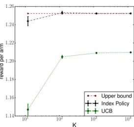
101 102 103 104 K 1.14 1.16 1.18 1.20 1.22 1.24 1.26 re w ard per ar m Upper bound Index Policy UCB
Figure 2.1: Upper bound and simulation results of MAB
the same distribution) with values ofαranging from 0 to 5 with a step size of 0.1 and then setαto the value that gives the best performance.
Figure 2.5.1 plots the reward per arm (expected total reward divided byK) againstK, forK =12,120,1200,12000. The red dashed line represents the upper bound computed usingP(λλλ∗). For each policy, circles show the sample mean of the total reward per arm, and vertical bars indicate a 95% confidence interval for the expected total reward per arm. The UCB policy’s sample means are connected by a dashed green line, and the index policy’s are connected by a dashed black line. Values are calculated using 5000 replications.
The index policy consistently outperforms the UCB policy. As K grows large, the confidence interval for the index policy’s total performance per arm overlaps with the upper bound, which numerically attests to the accuracy of Theorem 1 and illustrates the rate of convergence.
2.5.2
Project assignment problem
In our second experiment, we consider the following finite-horizon restless bandit prob-lem: suppose a team has K ongoing projects andm = bK/5c engineers who can work on any single project at a time. The manager of the team decides which projects to pri-oritize on a weekly basis. The state space of each project is the set of positive integers. Every project starts at the state of 1. The state of a project can either remain unchanged or can increment by 1 as we move to the next week. When an engineer works on a project in statesfor a week, it moves to the next state with probability p1(s); otherwise,
it transitions to the next state with probability p0(s). Each project can be worked on
by at most 1 engineer. When a transition happens, the team collects a reward which is a function of the current state. All the states have the same reward 1 except the final state which has a reward of 50. The manager’s goal is to maximize the total expected reward over a horizon ofT =5 weeks. Here we set p1(s)= 0.9−0.6s/T fors<T, and
p1(s)=0.05 for s= T. We setp2 =0.16p1.
For comparison we use Whittle’s index policy [48] and a randomized policy that selectsmprojects randomly at every time step. To apply Whittle’s index policy which is for infinite horizon setting, we convert the problem to a infinite horizon problem by adding an absorbing state for timeT onwards, and make all the state at timeT transit to this absorbing state with probability 1.
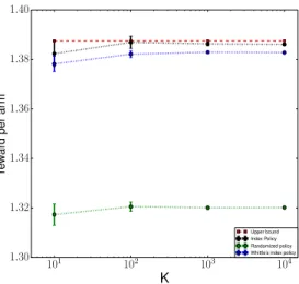
Figure 2.5.2 presents the outcome of the experiment at K = 10,100,1000,10000. Again we plot the number of projects against the per arm reward. We use red dashed line to represent the upper bound. The green dashed line shows the result of the ran-domized policy, which perform significantly worse than the other two. The index policy is represented by the black dashed line and the Whittle’s index policy is represented by the blue dashed line. The index policy out-performs the Whittle’s policy and converges
101 102 103 104 K 1.30 1.32 1.34 1.36 1.38 1.40 re w ard per ar m Upper bound Index Policy Randomized policy Whittle’s index policy
Figure 2.2: Upper bound and simulation result of project assignment problem
to the upper bound. Whittle’s policy is sub-optimal as it considers average case over time. Hence it tends to allocate more resources to projects which are in state 5 which has a very low probability of getting a large reward, while the optimal thing to do is to allocate resource to arms that are that a state with lower value but has a much higher probability of obtaining some reward.
2.5.3
Subset selection problem
In the third experiment, we consider a subset selection problem in ranking and selection whose goal is to identify mbest designs out of K designs, each with some underlying distributionθx. This problem is considered in [9] as well as [33]. We assume ¯mparallel computing resources are available; at each time step we select ¯m out of K design to evaluate. After T rounds of evaluation, we select m best designs. In this numerical study, we setT =4, mK = 0.3 and mK¯ =0.5. We consider the situation when the outcomes of evaluation are binary, but note that our model can handle any real-valued outcomes.
Below is how we formulate this problem as an RMAB: maximize πππ∈Π E πππ T+1 X t=1 Rt St,At subject to Pπππ(|At|=m)=1, fort= T +1, Pπππ(|At|=m¯)=1, for 1≤t ≤T, (2.19)
whereRt(St,At) = 0 whent ≤ T, andRt(St,At) = PK
x=1E[θx|St,x] whent = T +1. We
start with a uniform prior for each design.
We compare the performance of our policy against theOCBA-mselection procedure proposed in [9]. Since [9] considers a slightly different setting in which a policy maker can evaluate a design more than once in a time step, we modify the procedure slightly to fit our setup: instead of sampling according to the number of times dictated by the algorithm, we rank the designs by their desired number of samples, and simulate the first ¯m of them. Moreover, we assign a positive sample and a negative sample to each of the design at the beginning of the simulation so that it starts with the same amount of information as our Bayesian setup. We also use the UCB policy as a standard of comparison. The implementation of the UCB policy is similar to the one in section 2.5.1.
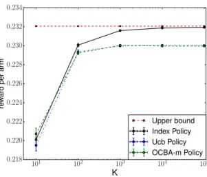
The simulation results show that all the three policies perform similarly when K
is small, with the OCBA-m policy having a slight edge for K = 10. From K = 100 onwards, the index policy consistently outperforms the other two. In addition, the gap between the upper bound and the index policy vanishes as K becomes large, while the gaps between the upper bound and the other two policies remain constant.
101 102 103 104 105 K 0.218 0.220 0.222 0.224 0.226 0.228 0.230 0.232 0.234 re w ard per ar m Upper bound Index Policy Ucb Policy OCBA-m Policy
Figure 2.3: Upper bound and simulation result of subset selection
2.6
Conclusion
In this chapter we propose an index-based policy for finite horizon RMAB problems that is computational tractable, and prove that it is asymptotically optimal in the same limit as considered by Whittle. We also show that the numerical performance of this index-based policy beats the state-of-art. For future work, we conjecture that our results, including the formulation of the policy and the asymptotic optimality, can be extended to the following situations:
1. Multiple actions associated with a state, instead of an active and a passive action in the current formulation;
2. A total budget constraint over the entire time horizon, in addition to a budget constraint at every time step.
CHAPTER 3
PARALLEL BAYESIAN POLICIES FOR FINITE MULTIPLE COMPARISONS WITH A KNOWN STANDARD
In this chapter, we consider an applied problem in simulation optimization: the multi-ple comparisons with a known standard (MCS). The problem is similar to an RMAB problem considered in Chapter 2 except that it allows multiple pulls per arm at a time. In this problem, one wishes to use simulation to determine, for each among a finite pool of simulating systems, which ones have an expected output measure that exceeds a known threshold. In this chapter, we use Bayesian statistics and dynamic programming to study how one should allocate simulate effort in the MCS problem, so as to best sup-port this final determination. This chapter is organized as follows: In Section 3.1, we do a light motivation and literature review; In Section 3.2 we formally state the problem; In Section 3.3, we provide a computationally tractable upper bound on the value of a Bayes-optimal procedure, and a method for computing this upper bound; In Section 3.4 we present a heuristic motivated by this upper bound, which is similar to the index-based policy proposed in Chapter 2 for RMAB, with the exception that it allows assignment of multiple resources to a system at a time; In Section 3.5 we present numerical results in which we demonstrate that the index policy performs close to an optimal policy; Lastly we present our numerical results and conclusion in Sections 3.5 and 3.6.
3.1
Introduction
The MCS problem arises in at least two distinct ways in simulation applications. First, it arises when determining which options perform better than some standard option whose performance is so well-estimated that it can be treated as known [36]. Second, it arises
when determining which options have a secondary performance measure that satisfies a constraint [2]. The MCS problem also arises outside of simulation, in crowdsourcing service centers like Amazon’s Mechanical Turk, when allocating a budget across work-ers who label items (e.g., images, documents), to best support accurate classification of these items [12].
We consider a variant of the MCS problem in which parallel computing resources are available. The growing availability of parallel computing resources presents new op-portunities to perform simulation analysis at larger scales, but also imposes constraints on the way simulation effort is allocated. In our model, simulation effort is allocated batch-sequentially: simulations are performed in batches, and we decide how many ad-ditional replications to perform for each system at the start of each batch based on the results of previous batches. We are given a fixed budget, specified as a number of par-allel computing resources and a number of batches, and our goal is to allocate these batches of simulation efficiently, so as to best allow correct classification of the systems once our simulation budget is exhausted.
We formulate the MCS problem in a Bayesian framework, and we measure the per-formance of a batch-sequential procedure by its average case perper-formance, averaging across problem instances drawn from the prior and across simulation noise. While the Bayes-optimal procedure is characterized by the dynamic programming equations [19], the curse of dimensionality makes solving this dynamic program computationally in-tractable for problems with many systems.
Rather than solving this dynamic program exactly, we provide a computationally tractable upper bound on its value. This allows us to evaluate the quality of sub-optimal heuristic policies relative to this upper bound. This provides guidance to the develop-ment and improvedevelop-ment of heuristic policies, in the form of information about the
opti-mality gap. The analysis technique used in this upper bound is a Lagrangian relaxation on the total number of simulations performed in any given batch. Using the Lagrange multipliers obtained from this relaxation, we also develop a heuristic policy, and use nu-merical experiments to demonstrate that it performs close to the upper bound on optimal in the problem setting studied.
This chapter builds on the previous work [49], which also considered the Bayesian MCS problem. That chapter considered the sequential setting, without parallel re-sources, and provided a computationally efficient method for computing the Bayes-optimal policy under two assumptions about limitations of sampling: that there is a time horizon that is random and exponentially distributed; or there is no time horizon, and we pay a fixed cost for each sample. Our current work differs from that work by considering parallelism, and by considering a fixed budget. While the infinite-horizon fixed-cost-per-sample model in [49] is quite natural for cloud computing settings, and the random exponentially distributed horizon is attractive for its computational tractability, using a fixed horizon is more natural than either model in [49] when allocating computing re-sources that are owned rather than rented. While we focus on the parallel setting and [49] focused on the sequential setting, our work can also provide an upper bound for the sequential setting with fixed horizon by setting the number of parallel nodes to 1.
For simplicity in this chapter, we consider only Bernoulli samples, with a linear loss function. However, the techniques developed in this chapter should also be adaptable to other parametric sampling distributions with conjugate priors, and other loss functions.
Our model assumes synchronous computations, in which we wait for all simulations in a batch to complete before starting the next batch. This approach is reasonable when the variability in the time to simulate a system is small enough to allow waiting until simulations finish before starting the next batch. Such assumptions are more commonly
met in controlled high-performance computing environments, and are less common in cloud computing environments. If computation time is highly variable, it may be more appropriate to model computation as asynchronous.
Our Lagrangian relaxation of a budget constraint in the MCS problem is related to Lagrangian relaxations in restless multi-armed bandit problems [48, 23]. Indeed, if one added an additional constraint that each system can be simulated at most once in any batch, then our MCS problem can be reformulated as a restless multi-armed bandit problem where we can pull multiple arms in each round: in this restless multi-armed bandit problem, each system is an arm, pulling the arm corresponds to simulating that system; the reward from this pull is the improvement in our ability to classify this sys-tem; and the number of arms we can pull in a round is the number of parallel resources. The restless multi-armed bandit framework of [48] is most well-known for allowing bandit arms to evolve when they are not pulled, but also allows multiple pulls per round. Our analysis can be seen as examining a generalization of restless bandits in which each arm can be pulled multiple times per round, and our heuristic policy can be seen as a generalization of the Whittle index policy to this setting.
Our use of a Lagrangian relaxation to study the Bayesian formulation of the MCS problem is also similar to [50], which used a Lagrangian relaxation to bound the value of the Bayes-optimal procedure for the ranking and selection problem.
While we consider the MCS problem in the Bayesian setting, much of the previous work on the MCS problem has considered non-Bayesian settings. This previous work includes the one-stage procedures by [37, 16], the two-stage procedures by [15, 7, 13], and work on indifference-zone ranking and selection (see the survey [32]). The more recent frequentist work includes [5] which provides a fully sequential procedure under stochastic constraint, and [26] which further allows correlation across systems.
In the version of the MCS problem that we consider, we emphasize that our standard has known value, and we seek to determine only whether each system is better or worse than this standard. We do not consider standards with unknown value, produce joint confidence intervals, nor select the best among those systems performing better than standard. This is in contrast with much previous work on multiple comparisons [36, 31]. The variant of the MCS problem that we consider has also been calledfeasibility determination[44].
3.2
Problem Formulation
We haveksystems, each of which can be simulated using a stochastic simulation. When we simulate system x∈ {1, . . . ,k}, we observe aBernoulli(θx) random variable,
indicat-ing the system’s performance in that simulation. We will think of an outcome of 1 as indicating the system succeeded in that simulation, and 0 as indicating failure. Although we expect that the methods we develop in this paper can be extended to simulations that generate non-Bernoulli samples, we focus on the Bernoulli setting here for simplicity. The sampling meansθx are initially unknown, and we wish to determine through sim-ulation, for each system x, whether θx is greater than some known threshold dx. This threshold may differ across systems.
We adopt a Bayesian formulation, in which we seek to do well on average with respect to a prior probability distribution over the unknown sampling meansθ1, . . . , θk.
We consider Bayesian prior probability distributions under which θx ∼Beta(α0,x, β0,x),
with independence across x, for some given values α0,x, β0,x. We assume a Beta prior
assumption allows our posterior distribution to remain Beta-distributed.
We performN batches of simulations, performing at mostmsimulations in parallel in each batch. At the start of each batchn= 1, . . . ,N, we choose the number of samples
zn,x to take from each system x, making sure to satisfy the constraintP
xzn,x ≤ m. This choice ofzn,x may depend upon the results observed from all previous batches. We then observe the number of successes from each systemx, which are conditionally binomial,
Yn,x|θx,zn,x ∼ Binomial(zn,x, θx).
We assume conditional independence of Yn,x across x and from all previous samples, givenθx andzn,x. This precludes the use of common random numbers, but is satisfied when using independent sampling. After observing this Yn,x, we update our posterior distribution onθxto obtain [14]
θx|z1,x,Y1,x, . . . ,zn,x,Yn,x ∼Beta(αn,x, βn,x),
whereαn,x = α0,x +Pn0≤nYn0,x can be interpreted as the effective number of successes from system x, and βn,x = β0,x+Pn0≤n(zn0,x −Yn0,x) as the effective number of failures. This posterior is independent acrossx.
We use dynamic programming to analyze this problem. To support this, for each x and n, we define the state variable Sn,x = (αn,x, βn,x). To streamline the discussion, we define αααn = (αn,1, ..., αn,k), βββn = (βn,1, .., βn,k), Sn = (Sn,1, ...,Sn,k),
and zn = (zn,1, . . . ,zn,k). Let Λn be the space in which Sn takes values, Λn =
n α0,1+ s1, β0,1+ f1, . . . , α0,k +sk, β0,k+ fk: sx, fx ∈Z+∀x, Pk x=1sx+ fx ≤mn o .
We stop sampling after batchNand decide, for each systemx, whether to labelθxas above or below the thresholddx. If we label it as above, we receive a reward ofθx −dx. Otherwise, we receive dx − θx. The total terminal reward is the sum of these rewards across the systems. As shown in [49], to maximize the conditional expected value of this
reward given what we know after our simulations are complete (which is summarized inSN,x), we should choose to receiveθx−dwhenever the conditional expected value of this rewardEθx−d
x|SN,xis positive, and to receivedx−θx when it is negative. When making decisions in this way, the conditional expected terminal reward received is
maxEθx−d x|SN,x,Edx−θx|SN,x = Eθx −d x|SN,x = αN,x αN,x+βN,x −dx . Summing this reward across systems x, our conditional expected terminal reward is
r(SN)= k X x=1 αN,x αN,x+βN,x −dx .
We optionally allow a cost cx ≥ 0 for each sample generated for system x, in the same units as the objective function. For example, if the reward is monetary, then the cost might be the payment made to a cloud computing service such as Amazon Ec2 or Microsoft Azure for the computer time required to run a simulation. If the computers are owned, rather than rented, then it may be appropriate to set cx = 0. Combining this optional sampling cost with the rewardr(SN) gives the conditional expected overall reward r(SN)− k X x=1 N X n=1 cxzn,x.
Our goal is to find an algorithm or policyfor choosing the samples to take, zn,x, so as to maximize the expected value of this reward. A policy is a rule for choosing how to allocate the next batch of samples, based on the results of the previous samples as sum-marized by Sn. Formally, a policy π is a sequence of mappings π = (π0, . . . , πN−1),
where πn : Λn 7→ Zk+ maps the state Sn to the action zn = πn(Sn), while satisfy-ing the constraint on the number of samples in each batch. The set of all policies is
Π =n
π =(π0, . . . , πN−1) :Pkx=1πn,x(S)≤m∀n=0, . . . ,N−1,S∈Λn
o
, whereπnx(S) in-dicate thexth component ofπn(S).
Each policy π induces a probability distribution over (S0,z0, . . . ,SN−1,zN−1,SN), which we callPπ. We letEπ indicate the expectation taken with respect to this probabil-ity distribution. We define,
Vnπ(S)=Eπ r(SN)− k X x=1 N X n0=n+1 cxzn0,x |Sn= S ,
for 0 ≤ n ≤ N, which is the conditional expectation of the future reward under policy π, starting from stateSat timen. We also define the value function, used below in our dynamic programming approach, as
Vn(S)= sup π∈Π
Vnπ(S).
The (unconditional) expected reward obtained underπisV0π(S0), and an optimal policy
π∗
is any for whichπ∗∈arg maxπ∈ΠV0π(S0).
The problem supπ∈ΠV0π(S0) is a Markov decision process with finite horizon and
finite state space, and its solution is characterized by the dynamic programming equa-tions. To apply dynamic programming, we first write down the dynamic programming equation, which is a recursive relation forVn:
Vn(Sn)= max zn+1:Pxzn+1,x≤m −X x cxzn+1,x+E[Vn+1(Sn+1)|Sn,zn+1] , 0≤ n≤ N−1. (3.1a) VN(SN)= k X x=1 αN,x αN,x +βN,x −dx . (3.1b)
Any policy whose actions achieve the maximum in (3.1a) is optimal [17].
We can use these recursive equations to computeVndirectly, first calculatingVN(SN) for all possibleSN ∈ΛN, and then proceeding in a backward recursion, using previously computed values of Vn+1(Sn+1) to calculate Vn(Sn) for all Sn ∈ Λn. Then, given these computed value functions, we can compute an optimal policy.
While this direct dynamic programming approach is theoretically well understand, it quickly becomes computationally intractable askgrows. This is because the state space
at timen, Λn, hasO((mn)2k) elements, and so storing the value function at all possible states has a memory requirement that scales exponentially ink. Computation also scales exponentially in k. This computational infeasibility due to the large dimension of the problem is generally referred to as the ”curse of dimensionality” [38].
The computationally intractability of computing an optimal policy whenk is large leads us to consider other characterizations that can be computed more easily. In the next section, we show how to compute an upper bound on the value of the optimal policy that scales linearly ink, rather than exponentially.
3.3
Upper Bound
In this section, we provide a computationally tractable upper bound on the value of an optimal policy. This bound can be used to calculate an optimality gap for any desired heuristic policyπ, by comparing the upper bound to an estimate of the heuristic policy’s valueVπ(S0) obtained from direct simulation. This in turn can be used to judge whether a
particular heuristic policy is good enough to be used in practice, or if more development (either of better heuristics or tighter upper bounds) would be worthwhile.
The main idea in our upper bound is to relax the constraints Pk
x=1zn,x ≤ m with a
Lagrange multiplier. As the first step, we introduce valuesλλλ = (λ1, ..., λN) ∈ Rk+. The
value λn will be the Lagrange multiplier for the constraintPk
x=1zn,x ≤ m. For eachλλλ,
define a modified value functionVnλλλ(Sn) via the following recursion:
Vnλλλ(Sn)= max zn+1∈{0,1,...,m}k n −X x cxzn+1,x+E h Vnλλλ+1(Sn+1)|Sn,zn+1 i −λn+1 k X x=1 zn+1,x−m o ,n≤ N−1, (3.2a) VλλλN(SN)= k X x=1 αN,x αN,x +βN,x −dx . (3.2b)