OpenCommons@UConn
OpenCommons@UConn
Doctoral Dissertations University of Connecticut Graduate School10-7-2019
Accelerating Graph Processing on Large-scale Multicores
Accelerating Graph Processing on Large-scale Multicores
Masab AhmadUniversity of Connecticut - Storrs, [email protected]
Follow this and additional works at: https://opencommons.uconn.edu/dissertations
Recommended Citation Recommended Citation
Ahmad, Masab, "Accelerating Graph Processing on Large-scale Multicores" (2019). Doctoral Dissertations. 2329.
Accelerating Graph Processing on Large-scale
Multicores
Masab Ahmad, Ph.D. University of Connecticut, 2019
ABSTRACT
With the ever-increasing amount of data and input variations, portable performance is becoming harder to exploit on today’s architectures. Computational setups utilize single-chip processors, such as GPUs or large-scale multicores for graph analytics. Some algorithm-input combinations perform more efficiently when utilizing a GPU’s higher concurrency and bandwidth, while others perform better with a multicore’s stronger data caching capabilities. Architectural choices also occur within selected accelerators, where variables such as threading and thread placement need to be decided for optimal performance. This paper proposes a performance predictor paradigm for a heterogeneous parallel architecture where multiple disparate accelerators are integrated in an operational high performance computing setup. The predictor aims to improve graph processing efficiency by exploiting the underlying concurrency variations within and across the heterogeneous integrated accelerators using graph benchmark and input characteristics. The evaluation shows that intelligent and real-time selection of near-optimal concurrency choices provides performance benefits ranging from 5% to 3.8×, and an energy benefit averaging around 2.4×over the traditional single-accelerator setup.
Multicores
Masab Ahmad
M.S, University of Connecticut, Storrs, CT, USA, 2016
B.E., National University of Sciences and Technology, Islamabad, Pakistan, 2013
A Dissertation
Submitted in Partial Fulfillment of the Requirements for the Degree of
Doctor of Philosophy at the
University of Connecticut
Copyright by
Masab Ahmad
Doctor of Philosophy Dissertation
Accelerating Graph Processing on Large-scale
Multicores
Presented by
Masab Ahmad, M.S., B.E.
Major Advisor
Omer Khan
Associate Advisor
John Chandy
Associate Advisor
Marten Van Dijk
University of Connecticut 2019
ACKNOWLEDGMENTS
I am very thankful to my advisor, Prof. Omer Khan, who steered me towards the right path during my PhD studies. Even during my personal struggles, he supported me with utmost sincerity. I am indebted to him for the knowledge and invaluable experiences I have gained during my PhD.
I would like to thank my former and current colleagues, Farrukh Hijaz, Syed Kamran Haider, Hamza Omar, Halit Dogan, Qingchuan Shi, Mohsin Shan, and Akif Rehman, for their continued support, and great friendship. Special thanks should go to Farrukh Hijaz and Syed Kamran Haider as I owe them a lot for mentoring me in my early years of my studies at the University of Connecticut.
I would like to acknowledge the funding received for supporting my PhD research from US National Science Foundation, the Naval Research Laboratory (NRL), Semiconductor Research Corporation (SRC), IBM Research, and NXP Semiconductors. I would specially like to express my appreciation to Brian Kahne of NXP Semiconductors for his continuous support on the development of the multicore simulator and workloads that I employed in my research. I would also like to thank Jos´e Joao of Arm Research, and Christopher Hughes of Intel Corporation for their valuable discussions and feedback towards the evolution of my research.
I also would like to thank my unconditionally loving and supporting family. Knowing that my parents, Zia and Rema Ahmad, and my siblings, Sohaib and Aleena Ahmad, always keep me in their prayers gave me great strength when I was under a lot of stress. I wouldn’t have been able to be where I am without their support and encouragements.
Last but not least, I am grateful to my wife, Fajar, for being beside me, with a great patience and support during the most stressful times. When I was almost always working, and busy, she was the
Contents
Page
List of Figures vii
List of Tables ix
Ch. 1. Introduction 1
Ch. 2. Multi-Accelerator System 6
Ch. 3. Performance Prediction Paradigm 8
3.1 Tuning the Intra- and Inter- Accelerator Choices . . . 8
3.2 Input (I) Variables . . . 10
3.3 Input Graph Expression using I Variables: . . . 12
3.4 Benchmark (B) Variables . . . 12
3.5 Benchmark Expression using B Variables . . . 15
Ch. 4. HeteroMap Decision Tree Model 18 4.1 Inter-Accelerator (M1) Model . . . 19
4.2 Intra-Accelerator (M2−20) Selection . . . 20
4.3 M Choice Selection Example . . . 25
Ch. 5. HeteroMap Framework Automation 28 5.1 Offline Learning Formulation . . . 28
5.2 Training of Models . . . 30
5.3 Online Evaluation . . . 31
5.4 Deep Learning Prediction Model . . . 32
5.5 Regression Prediction Model . . . 33
Ch. 6. Methodology 35
6.1 Accelerator Configurations . . . 35
6.2 Benchmarks . . . 36
6.3 Processing Metrics . . . 37
Ch. 7. Evaluation 39 7.1 Selecting a Learning Model . . . 39
7.2 Performance Variations . . . 41
7.3 Understanding Energy & Utilization Variations . . . 43
7.4 Changing Fixed Accelerator & Memory Sizes . . . 43
7.5 The Impact of Re-Learning . . . 47
7.5.1 Training Evaluation . . . 48 Ch. 8. Related Work 50 Ch. 9. Conclusion 52 Ch. 10. Future Work 53 Ch. 11. Associated Publications 55 Bibliography 59
List of Figures
Page
1.0.1 How input graph variations exhibit different performance within and across
under-lying accelerators in SSSP. . . 3
1.0.2 Multi-accelerator system example with the run-time performance predictor for graph benchmarks and inputs. . . 5
2.0.1 Machine choices (M) for GPUs and multicores. . . 7
3.5.1 Discretization of (B) variables for SSSP-Bellman-Ford (SSSP-BF).. . . 17
4.2.1 Decision Tree Heuristic Model flow for SSSP-BF and SSSP-Delta with the USA-Cal input graph. The proposed model predicts and selects nineM choices. . . 26
4.3.1 HeteroMap Framework Flow for the Multi-Accelerator Architecture. . . 27
5.1.1 Example synthetic benchmarks generated. . . 30
5.3.1 Neural Network showing network parameters. . . 32
5.4.1 Non-Linear Regression Equation. High-profile variables and associated trends in input dependence on output thread selections also shown. . . 33
7.2.1 Scheduler Comparisons for Graph Workload-Input Combinations (All results normalized to the GTX750Ti GPU implementation) (Higher is worse). . . 42
7.2.2 Energy benefits averaged for various inputs for a given benchmark. (Xeon Phi vs. GTX 750Ti). All results normalized to the maximal energy used for anyB−I combination. . . 43
7.4.1 Scheduler Comparisons for various Graph Workloads-Input Combinations (All results normalized to the GTX970Ti GPU implementation) (Higher is worse). Note that Optimal Choices change when compared to the GTX750Ti in Figure 7.2.1. 44 7.4.2 Geomean results averaged for different inputs for each benchmark for the 40-core CPU. All results are normalized to the GPU implementation. . . 45
7.4.3 Memory size variations for different machine combinations. The x-axis varies memory sizes for a multi-accelerator system, while the y-axis shows normalized
List of Tables
Page
3.1.1 Input Datasets. . . 11
6.2.1 Primary Accelerator Configuration. . . 36
6.2.2 Synthetic Input Datasets. . . 37
7.1.1 Learning Model Strategies. Speedup shown over the GTX-750 GPU. . . 40
7.5.1 Re-Learning Performance. Compared with the baseline case of the GTX-970 as it had better performance. . . 48
7.5.2 Sensitivity to Training on Deep. - 128. Speedup shown over the GPU. Using all synthetic graphs provide the speedup shown in Table 3. . . 49
Introduction
Target applications that utilize graph processing are rising in a plethora of architectures [1, 2]. Future HPC datacenters are expected to have heterogeneous connected accelerators, with Cray and NVidia already edging on similar ideas [3,4]. It has been indicated in prior works that graph analytics pose limitations when executed on a single accelerator setup [5] [6]. Thus, this paper proposes a multi-accelerator setup to situationally adapt the graph problem and input to the right machine and its concurrency configurations. To understand this problem, consider the iterative Bellman-Ford algorithm and its variants finding shortest paths. Such a graph algorithm lends itself for data-parallel execution since it easily allows graph chunks to be accessed in parallel. Hence, such an algorithm performs well on a GPU, since it exploits massively available threading to exploit parallelism [7]. On the other hand, algorithms such as Triangle Counting are not as parallel, and comprise of reductions on vertices that result in complex data access patterns. These access patterns lead to increased data movement and synchronization requirements [8]. Multicores perform well in such cases as they incorporate caching capabilities for efficient data movement and thread synchronization [9]. These variations solidify theneed for diverse types of accelerators in a setup
2
executing graph analytic workloads.
Taking this problem into context, this paper takes a heterogeneous architecture that constitutes both types of competitive multicore and GPU accelerators connected under their own discrete memories. This setup exposes concurrency choices to graph applications, thus catering for the missing throughput and reuse capabilities in GPUs and multicores. Performance variations occur not only due to changes in benchmark characteristics, but also input changes within a benchmark, as well as different mappings of graph analytic benchmark-input combinations on different accelerators. These choices do not exist in a single accelerator setup. Algorithmically, in the presence of expensive synchronization on shared-data or indirect memory accesses, GPUs cannot perform as well as multicores. Multicores possess hardware cache coherence and a complex cache hierarchy to exploit performance in such cases [10]. In various cases, the massive throughput of the GPU, or the data reuse of the multicore needs to be constrained to reduce stress on the memory system and data communication. One way to manage this is to spawn less threads in the workload [7]. Thus, choices occur bothwithinandacrossaccelerators, for different benchmarks and inputs.
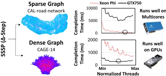
Input dependence is known to play a big role in graph analytic performance [11] [12]. An example of such a trade-off is shown in Figure1.0.1, which shows an OpenTuner optimized [13]
∆-stepping single source shortest path (SSSP) algorithm [14] running a sparse and a dense graph on an Intel Xeon Phi 7120P multicore, and an Nvidia GTX-750TI GPU. Threads are varied from minimum total available threads to maximum total threads for both accelerators, and are normalized on the x-axis, while the y-axis shows completion time. The two accelerators are categorized as competitive as they possess similar compute capabilities.
The multicore performs better than the GPU for the sparse road network [15], as a higher graph diameter results in longer dependency chains that determine the optimal path between source and destination vertices. This linked traversal leads to more complex data access patterns that are more expensive on the GPU, as it does not possess the addressing capabilities to perform such complex
0 5000 10000 15000 0 20 40 60 80 Xeon Phi GTX750
Sparse Graph
CAL-road-network Runs well on GPUs Runs well on Multicores C o m p le ti o n T im e ( m s) C o m p le ti o n T im e ( m s) 0 5000 10000 Normalized Threads Min Max 0 1000 2000Dense Graph
CAGE-14S
S
S
P
(
∆
-S
te
p
)
Figure 1.0.1: How input graph variations exhibit different performance within and across underlying accelerators in SSSP.
data accesses. Moreover, the different phases in∆-stepping result in more divergence and complex indirect addressing, which adds to GPU overheads. The multicore in this scenario performs several orders of magnitude faster than the GPU. The CAGE-14 graph [16] has a lower diameter, and thus requires less iterations to converge. Due to high density of edge connectivity, it lends itself to map optimally on a GPU. Larger available core and thread counts in GPU allow it to outperform the multicore by 3×. The GPU fares well in this case as they possess the capability to spawn thousands of threads without having to enforce many barrier synchronization calls. Even when the optimal accelerator is selected, there are a slew of machine choices within the accelerator to choose from. In the case of CAGE-14 graph, intermediate threading performs best on the GPU, as spawning more threads raises stress on the GPU’s already small cache system. This exhibits the vastness of the dimensionality of the input problem space, as various benchmarks and inputs may constitute different characteristics, making manual tuning difficult. Machine choices within and across accelerators therefore need to be tuned based on different inputs to achieve optimal performance. Moreover, for different benchmarks, the patterns that lead to concurrency and data accesses also vary across graph analytics, which further motivates the need to tune this accelerator
4 choice space.
This poses several questions: What patterns in graph benchmarks and inputs lead to best ex-ploitation of concurrency within and across GPUs and multicores? What are the architectural differences in these machines that lend them for mapping to the diverse benchmark-input com-binations? What are the run-time concurrency trade-offs of using one accelerator over another in a heterogeneous setup? Benchmarks and inputs reveal accelerator choices due to their direct correlations with the optimal architectural choices. Thus, graph benchmark and input choices need to be exposed systematically, after which a high level intelligent predictor tunes the accelerator choices. However, due to the increased high-dimensional space complexity and non-linear aspects of having multiple accelerators and their intra-concurrency choices, selecting the right choices becomes a hard problem.
This paper proposes a novel performance predictor framework,HeteroMap, which integrates benchmark and input choices to do dynamic selection of parameters within and across accelerators. The prediction framework captures program characteristics by intelligently discretizing graph benchmarks and inputs into easily expressible representative variables. Mappings of benchmark and input representations to inter- and intra-accelerator choices are done using a decision tree analytical model. The proposed analytical model is further automated using machine learning to amortize costs associated with the large graph algorithmic choice space. The automated model is trained using synthetically generated graph benchmarks [17,18], and inputs [19,20]. For a variety of graph analytic benchmarks executing real-world inputs,HeteroMapprovides performance benefits ranging from 5% to 3.8×when compared to a single GPU-only or multicore-only setup.
Multi-Accelerator
Architecture
Cache Coherence No Coherence Better Hierarchy Large Registers More Threads Less ThreadsMulticore
GPU
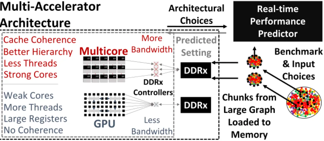
More Bandwidth Less Bandwidth DDRx Controllers Strong Cores Weak Cores FP FP FP FP FP FP FP FP FP FP FP FP FP FP FP Chunks from Large Graph Loaded to Memory DDRx DDRx Architectural Choices Benchmark & Input Choices Real-time Performance Predictor Predicted SettingFigure 1.0.2: Multi-accelerator system example with the run-time performance predictor for graph benchmarks and inputs.
Chapter 2
Multi-Accelerator System
The target system utilizes discrete GPU and multicore accelerators. The setup considers either a weaker NVidia GTX-750Ti GPU or a stronger NVidia GTX-970 GPU, but not both at the same time. We also consider a weaker Intel Xeon Phi 7120P multicore or a stronger 40-core Intel Xeon E5-2650 v3 multicore. All multicore-GPU combination pairs are considered to analyze the inter-and intra-accelerator design space. This multi-accelerator system is used as a prototype to convey the underlying idea of mapping architectural choices using graph benchmarks and inputs. Figure1.0.2
depicts an example multi-accelerator system showcasing a GPU and a Xeon Phi multicore with GDDR5 memories, as well as various architectural differences between associated accelerators. As memory size changes require architectural reconfigurations, evaluations are done on fixed memory sizes for each target accelerator. The design space of various combinations of memory sizes is also studied to analyze how main memory size changes affect performance in accelerators.
Input graph chunks are loaded in the accelerator’s DDR memory for processing. The system is used in a way that graph benchmark-input combinations are loaded and executed with the appropriate architectural choices for individual accelerators with the discrete memory size constraint. In a
M
u
lt
ic
o
re
H
a
rd
w
a
re
C
h
o
ic
e
s
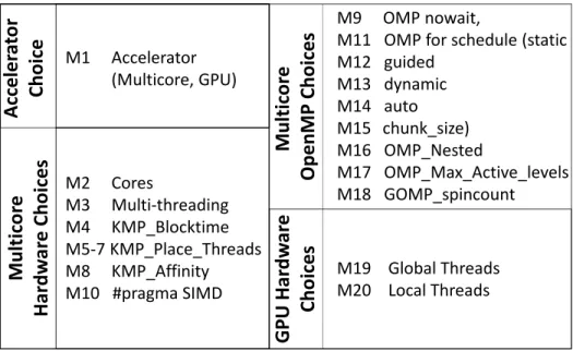
M9 OMP nowait,M11 OMP for schedule (static M12 guided M13 dynamic M14 auto M15 chunk_size) M16 OMP_Nested M17 OMP_Max_Active_levels M18 GOMP_spincount M19 Global Threads M20 Local Threads M1 Accelerator (Multicore, GPU) M2 Cores M3 Multi-threading M4 KMP_Blocktime M5-7 KMP_Place_Threads M8 KMP_Affinity M10 #pragma SIMD
M
u
lt
ic
o
re
O
p
e
n
M
P
C
h
o
ic
e
s
G
P
U
H
a
rd
w
a
re
C
h
o
ic
e
s
A
cc
e
le
ra
to
r
C
h
o
ic
e
Figure 2.0.1: Machine choices (M) for GPUs and multicores.
real-time context, it is harder to allocate graph chunks and process them as larger graphs do not fit in main memory. Hence, chunks from larger graphs are thus extracted temporally using a state-of-the-art Stinger framework [21], and streamed in the accelerator’s memory to be processed. The prediction paradigm takes in graph chunk characteristics, and predicts optimal architectural concurrency parameters for each chunk.
Chapter 3
Performance Prediction Paradigm
Graph inputs consist of vertices,V, which are connected to other vertices via edges, E. Graph benchmarks loop around outer vertices and inner edges, and different phases in workloads have different complexities and have diverse data access patterns. Due to data access and synchroniza-tion pattern differences in graph inputs and workloads, different benchmarks and inputs perform optimally on different machines with different intra-accelerator settings. The multi-accelerator architecture in Figure1.0.2exposes theseintra- and inter- accelerator variations, and we create a knowledge base from benchmarks and inputs that can be mapped to these machine choices.
3.1
Tuning the Intra- and Inter- Accelerator Choices
Various capabilities in GPU and multicore accelerators allow improved performance extraction for specific graph benchmark and input characteristics. This trade-off between accelerators is depicted as M1in Figure 2.0.1, where either a GPU or a multicore can be selected. In GPUs, massively available threading hides data access latencies to deliver high throughput execution.
This occurs in data-parallel workloads with small dependency chains and less shared data, and thus GPU accelerators must be selected for such cases. Although GPUs fare well with highly data-parallel execution, they under-perform when benchmarks have complex data access patterns, costly synchronization, and inter-thread data movement. Moreover, even in data-parallel workloads, the threading and throughput of a GPU may need to be constrained due to varying input sizes and densities to reduce stress on the memory system for optimal performance. This createstwo choices within a GPU: Global threading, which distributes threads across the GPU chip,
and Local threading, which specifies the thread count on a GPU core. These choices are
listed in Figure2.0.1as GPU hardware choices,M19−20.
Multicores perform well for complex data access patterns by taking advantage of their cache reuse and cache coherence capabilities. Therefore, multicores should be selected if there is ample shared data. Multi-threading usage and placement intra-choices depend on the input graph char-acteristics such as edge density. Specifically formulticore threading,KMPaffinity/place threads
are thread placement hardware choices in Figure2.0.1, while # pragma simdcontrols SIMD usage. Thread placement may be compact or loose, and is important for data movement along with core and cache utilization. For example, threads may want to use cache slices of unused cores, which can be enabled by placing threads in the center of unused core clusters. This improves performance by reducing data movement and synchronization costs as threads are placed closer to the residing data.KMPblocktimeis another parameter, which defines the time a thread waits before going to sleep. This is helpful during contention and load imbalance, as threads can go to sleep before polling on contended data.
Other parameters, such as those in the OpenMP paradigm, also have non-linear relationships with benchmarks and inputs, and are used to improve shared data reuse and movement costs.Scheduling variables in OpenMPinvolve dynamic scheduling, which control work distributions across parallel regions. Scheduling is controlled byOMP for schedule, which is tasked withstatic, dynamic,
10
guided, or autochoices, and data tile/chunk sizes. Data scheduling is related to access patterns, which require dynamic scheduling on read-write shared data. This mitigates contention and data movement overheads [22]. Additional parameters such asOMP Nestedexploit nested parallelism within loops, while OMP Max Active Levels states how many levels of parallelism can be nested. GOMP Spincountdefines how long threads actively wait for OpenMP calls. Larger times with this variable may be used to increase waiting times for threads if there is high contention. These OpenMP parameters are denoted asM9, M11−18, and are listed in Figure2.0.1.
TheM variable space is a function of the target benchmark and associated graph input, and this is the formulation required to achieve tuning ofM parameters. All choices symbolize a non-linear mapping between benchmarks and graphs, andM choices. Thus, we create a benchmark and input graph representation space, denoted byB andI respectively. To minimize performance, a tuple vector,X, is constructed that takes benchmark choicesB~, input choicesI~, and accelerator choices
~
M, to minimize performance in the proposed architecture:X(~M) =M inP erf(B, ~~ I). The function,
M inP erf()is the proposed configurator that findsM choices. To properly relate benchmark and
inputs withM choices,B andI variables need to be extracted and classified for tuning. The next sections first describeB, Ivariables in the context of how they are expressed, and their relationships with machine choices.
3.2
Input (I) Variables
The most relevant input variables are graph size using vertex counts (I1) and edge density (I2), which specify the size of the graph and the density of computations. Higher graph sizes and densities can be divided into more threads, thus thread count selections in accelerators are directly correlated withI1andI2. The maximum edge count of any vertex in the graph (I3) is also relevant
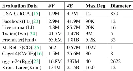
Table 3.1.1: Input Datasets.
Evaluation Data #V #E Max.Deg Diameter
USA-Cal(CA)[15] 1.9M 4.7M 12 850 Facebook(FB)[23] 2.9M 41.9M 90K 12 Livejournal(LJ) 4.8M 85.7M 20K 16 Twiter(Twtr)[24] 41.7M 1.47B 3M 5 Friendster(Frnd) 65.6M 1.81B 5.2K 32 M. Ret. 3(CO)[25] 562 0.57M 1027 1 Cage14(CAGE)[16] 1.5M 25.6M 80 8 rgg-n-24(Rgg)[23] 16.8M 387M 40 2622 Kron.-Large(Kron) 134M 2.15B 16.0 12
as it defines how much deviation there is in edge connectivity from the average density usingI2. This is used to define average per-thread work, as well as divergence in work between threads. Higher or lower per-thread work is used to decide how much local threading and/or SIMD to use, while work divergence is used to optimally place threads, in a selected accelerator. Graph diameter (I4) specifies the largest connectivity distance between any two vertices, specifying dependency chain sizes between vertices in a graph. I4is obtained alongside input graphs or using run-time approximations [26]. This in turn expresses how much the memory system is going to be stressed during execution, as longer vertex dependency chains need to be remembered in memory. I4is helpful in deciding which type of memory system needs to be tuned for an input graph.
All input variables are also easily expressible in percentages, as maximum vertex and edge count, maximum degree, and diameter, are known in literature [17]. These proposedI variables are used to classify a real input graphs to expose input variations, shown in Table3.1.1. These range from sparse road networks, social networks, to dense mouse brain graphs.
12
3.3
Input Graph Expression using I Variables:
I variables are deduced from graph data and are shown in Figure3.3.1a. These representations are simply obtained by normalizing the input graph’s characteristic data, and setting it to a value between 0 and 1, with increments of 0.1, depending on the acquired value. I variables are normalized by comparing the input graph characteristics to the maximum values available in literature [27,14] for these variables. Normalization is necessary, as these characteristics need to be compared to each other to predict inter- and intra-accelerator choices. Furthermore, as graphs have extremely large variations among themselves in terms of characteristics, a logarithmic normalization is applied to further smoothenI values. Using the USA-Cal input graph as an example to computeI variables, vertex and edge counts in USA-Cal are low compared to the largest graphs such as Friendster. HenceI1,2are set to 0.1 for USA-Cal, but 0.8 for Friendster. As the maximum degree of USA-Cal is also extremely low compared to the largest available degree in Twitter (which is 1),I3is set as 0 in this case. However, its diameter is close to the highest available (850 is close to the largest diameter of 2622 for the Rgg graph). Therefore, we setI4as 0.8 for USA-Cal and 1 for Twitter, and 0 for all other graphs.I variables for other input graphs are extracted similarly and shown in Figure3.3.1a.
3.4
Benchmark (B) Variables
In parallel graph algorithms, the outermost loop is parallelized, and traverses graph vertices in various phases such as highly parallel vertex division and pareto fronts, or less parallel reductions and push-pop phases. An algorithm may consist of multiple phases, where phases are separated by global thread barriers. Inner loops traverse edges, where data is addressed either directly using loop indexes, or indirectly using complex pointers. Data may be either shared as read-only or as
FB LJ Twtr Frnd CO CAGE Rgg Kron CA I1 I2 I3 I4 0.1 0.1 0 0.8 0.1 0.2 0.1 0 0.2 0.3 0.2 0 0.7 0.7 1 0 0.8 0.8 0.1 0 0 0 0.1 0 0.1 0.2 0.1 0 0.5 0.4 0 1 1 1 0 0 USA-Cal (CA) I1= 0.1 I2= 0.1 I3= 0 I4= 0.8 In p u t G ra p h V a ri a b le s I1 Vertex Count
# of vertices in the graph
I2 Edge Count
# of edges in the graph
I3 Max. Edge Count
Highest edge count of a vertex in the input graph
I4 Diameter
Greatest distance between any two vertices
Input Graph Classification using I variables CAGE-14 (CAGE) I1= 0.1 I2= 0.2 I3= 0.1 I4= 0
(a) Input variables for real graphs.
SSSP-Delta BFS DFS PageRank-DP PageRank Tri.Cnt. Comm. Conn. Comp. SSSP-BF B1 B2 B3 B4 B5 B6 B7 B8 B9 B10B11 B12 B13 B1 B2 Vertex Division Pareto V e rt e x P ro ce ss in g / S ch e d u li n g C o m p . T y p e M e m o ry A cc e ss % program in vertex division % program in pareto fronts B3Pareto-Division % program in divided paretos B4Push-Pop % program in Push-Pops B5Reduction % program in reductions B6Floating Point % floating point data B8 B9 Indirect Read-only Data % complex pointer addressing % read-only program data B10 Read-write Shared Data % shared read-write program data B11Locally Accessed Data % locally accessed data B12Contention
% data contended via atomics
B7 Data Driven
% accesses addressed by data
# global barriers per iteration
B13Barriers
Benchmark Representation using B Variables
S y n ch ro n iz a ti o n D a ta M o v e m e n t D a ta M o v e m e n t
(b) Benchmark variables and representations.
read-write, and may require atomic updates. Read-write shared data may require local computations with either fixed point or floating point (FP) requirements to calculate output values to write into global data structures. These generic primitives are used to generateB benchmark variables. In this work, variablesB1−13define structural differences within graph-specific data structures and parallel phases, which are critical components in predicting machine choices.
Initial B variables are derived using outer loop parallel primitives. The outer loop may be data-parallel using Vertex division (B1), lending itself easily for execution with a larger number of independent threads. Pareto (B2) execution can also be applied on outer loops, where chunks of vertices mapped to threads statically increase with workload progression. These Pareto phases may also dynamically increase vertices in threads (B3). Graph workload phases may also take the form of Push-PopB4accesses, which add certain ordering constraints for processing. This in turn enforces dependencies, leading to complex data access patterns. Like Push-Pop accesses, Reductions (B5) contain more sequential work than other phases, and involve synchronization primitives with atomic
14 operations. (B4) and (B5) phase types complicate data access and parallelism, leading to thread divergence. Therefore, GPUs may under perform for such scheduling patterns [28]. However, (B1−3) lend themselves for high parallelism on the GPU. These variables are important, as they describe how much each phase constitutes a benchmark. Thesevertex processing and scheduling variables(B1−5) are mutually exclusive, as programs are divided into phases. For example, a program may consist of 80% vertex division, and a 20% reduction phase. A programmer sets these variables by finding out how much a phase constitutes each benchmark.
Compute typewithin phases may be FP computations done by the inner loops of workload phases. These FP computations determine if dedicated hardware units need to be exploited. This is shown by how much program data is specified as FP (B6), which trades-off accelerators, as some accelerators may have more FP capabilities than others. For example, if 20% of program data requires FP, then (B6) is set as 0.2. FP operations perform optimally on multicores if they are in a dense format to exploit SIMD capabilities. Therefore, knowing how much FP computations are needed can decide in mapping a benchmark to either a multicore or a GPU.
In terms of memory access patterns, addressing is either done with loop variables (B7), or by complex indirect addressing such as double pointers (B8). Complex addressing primitives are better handled in multicores as they possess larger caches to hold addressing metadata, and have faster ways of resolving complex pointers and addressing. Indirectly accessing and reusing data via addressing in the cache does not fare well with GPUs as they do not have the capabilities or enough cache sizes to hold such contents. A programmer sets (B7,8) by viewing what percentage of data is accessed indirectly, or by using loop indexes.
Runtime data movementis also diverse, and takes the form of read-only shared data (B9), read-write shared data (B10), and locally accessed data (B11). (B9−10) fare well on multicores as they have cache management mechanisms for efficient data movement between cores. (B11) is data that is locally operated in thread registers, where it depends on the accelerator’s cores on how
fast they process local computations. Each of these variables is expressed by the programmer as a percentage of the total accessed data.
Shared data may also require updates withsynchronization(B12), where (B12) is viewed as the percentage of data requiring locks, as certain accelerators may have better performing atomics than others. The number of barriers in a workload separating phases (B13) also causes variations. If there are more locks and barriers in a benchmark, then it produces more opportunities for inter-thread communication to cause bottlenecks and load imbalance. (B13) is specified as the number of barriers between phases, and each barrier increments (B13) by 0.1, per iteration.
(B1−5) are considered as independent variables. Although the interactions of remaining
B variables are complex, these variables are not considered mutually exclusive. All benchmark variables are also easily expressible in percentages. The programmer specifies whichB variables are interesting in a given benchmark. For simplicity, this section first uses aXrepresentation to signify whether eachB variable is specified or not in a benchmark. This classification is shown in the subsequent subsection.
3.5
Benchmark Expression using B Variables
Now that benchmark variables are defined, these variables can be used to classify real graph workloads. Graph workloads are thus acquired from a variety of benchmark suites, further specified in Section 6.2. These benchmarks are also listed in Figure 3.3.1b, with the Xrepresentations showing if aB variable is used in a benchmark. Based on compile-time information about loops and inputs, loop indexes and data structure sizes are inferred, and are used to approximate relative strengths ofB variables. As multicore and GPU versions of benchmarks use the same algorithms, theirB variable classification remains the same.
16 Taking the case of SSSP-BF as an example, the only parallelization applied is vertex division, which enables B1to be set asX. If the SSSP-Delta workload is used then parallel buckets are used to push and pop edges, settingB4asX. The GAP version also uses a reduction to select a bucket to use in subsequent iterations, which setsB5asX. In terms of program phases, the general distribution is that workloads use data-parallel vertex divisionB1along with reductionsB5. BFS uses only Pareto-divisionB3, and DFS uses only Push-PopB4, as workload phases only contain one phase of these types. All workloads have data-driven accessesB7, and read-write shared data
B10. DFS and Conn. Comp. have complex indirect data accesses, which are due to queuing and data-manipulated addressing, and these setB8toX.
B variables are percentages of program sections or percentages of data types used. These variables need to be normalized because simpleXrepresentations do not show intensities of each
B variable. B variables are depicted within a range of 0 and 1, with increments of 0.1. Finer increments may be applied, however we keep the model simple by not using very fine increments. As graph workloads consist of only phases separated by barriers, values for B1− 5variables for phases add to 1 for all benchmarks. To assign values for more than one B1−5variables in a benchmark (e.g. a workload having both Push-Pop and Reduction phases), the programmer decides approximately how much % code is in each phase. The programmer can statically view data structures to assign how much % of the structures fall in each of the remaining variableB6−12
categories. By specifyingBvariable values between 0 and 1, the programmer assigns percentages to variables, therefore properly assigning benchmark characteristics.
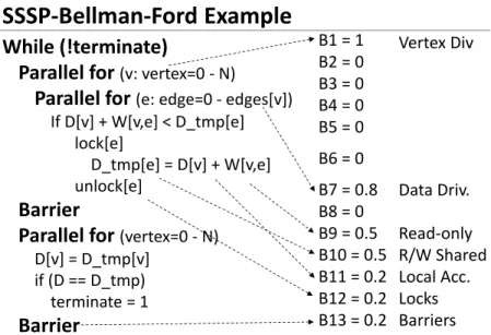
As an example, we take SSSP-BF to show this discretization, with its pseudocode shown in Figure3.5.1to visualizeB variables. As all of the program code in SSSP-BF only uses vertex division to parallelize outer loops, thusB1is set as 1 in Figure3.5.1, while the remainingB2−5are set as 0. B6is set as 0 because SSSP-BF does not utilize FP operations. Most of the data accesses are done using loop indexes, such as accesses forD tmp[],D[], andW[]arrays, therefore setting
SSSP-Bellman-Ford Example
.
While (!terminate)
Parallel for (v: vertex=0 - N)
Parallel for (e: edge=0 - edges[v])
If D[v] + W[v,e] < D_tmp[e]lock[e]
D_tmp[e] = D[v] + W[v,e] unlock[e]
Barrier
Parallel for (vertex=0 - N)
D[v] = D_tmp[v] if (D == D_tmp) terminate = 1Barrier
B1 = 1 B2 = 0 B3 = 0 B4 = 0 B5 = 0 B6 = 0 B7 = 0.8 B8 = 0 B9 = 0.5 B10 = 0.5 B11 = 0.2 B12 = 0.2 B13 = 0.2 Vertex Div Data Driv. Read-only R/W Shared Local Acc. Locks BarriersFigure 3.5.1: Discretization of (B) variables for SSSP-Bellman-Ford (SSSP-BF).
B7to 0.8. B8is set to 0 as there are no indirect accesses. Approximately half of the program data is composed of the input graphW[], which is read-only by all threads. The other half are the distance arrays (D tmp[]andD[]), which are read and written frequently by all threads. This setsB9and
B10to 0.5 each. Local computations are done onD tmp[], which constitutes approximately 20% of program data, hence this setsB11to 0.2. Locks are also applied only on theD[]array, which is half the size of the two distance arrays combined, and there are two barrier calls in the benchmark. This setsB12andB13to 0.2. Now thatB, I variables are set, relationships betweenB, IandM
Chapter 4
HeteroMap Decision Tree Model
Patterns ofM mappings allow visualization of accelerator choices withB and I variables. For example, benchmarks utilizing Push-Pop (B4) phases are expected to perform better on multicores than on GPUs. This is due to better data movement capabilities in multicore cache hierarchies, as well as better core performance for queuing operations. On the other hand, benchmarks with high data-level parallelism and local thread computations are expected to perform well on a GPU. This is because GPUs possess more threads to exploit available parallelism, and large register files to hold local computations. These relationships betweenB, I andM variables are used to create a simplified analytical decision tree model.
This section proposes a decision tree heuristic that analytically minimizes the choice space problem for performance (and energy if needed). Decision trees are easily readable and tunable, and thus allow for manual modeling. This model is expressed as an inter-accelerator model to first select an optimal accelerator, and then an intra-accelerator model to select concurrency choices within the accelerator. However, with 13B variables, 4I variables, and 20M variables, the resulting choice space consists of thousands of combinations to select from. Hence, to simplify the prediction model,
we only look at the most important variables that affect eachM parameter. The completeM model is provided as a C/C++ program in the URL provided1.
4.1
Inter-Accelerator (
M
1
) Model
A 3-layer manually constructed decision tree is formulated, selecting an accelerator based on (B, I) combinations. As the complete decision tree is too large, we describe a few partial decision examples. For example, if a combination hasB1orB2orB3each with a value greater than 0.5, meaning it has lots of vertex level parallelism, then a GPU is chosen as it exploits this available parallelism. This allows workloads such as SSSP-BF and BFS to run on the GPU. On the other hand, if a benchmark has serial Push-Pop accesses (B4) with a high graph density, then the multicore is selected as it performs well on Push-Pop accesses with the dense graph fitting in its local caches. In another example, if a benchmark has a high value ofB5(reductions) with some FP (B6), and negligible local computations (B11), then the GPU is selected. This is because GPUs perform well with reductions having low local computations, meaning the small GPU threads can make fast progress using their small caches.
The multicore is selected for the case with reductions (B5) and read-write shared data (B10). This is because the cache capabilities in multicores allow faster operations on shared data, while synchronization primitives required for reductions on vertices also perform well due to faster inter-thread communication abilities. For large graphs withI1>0.5, benchmarks with indirect addressing are also run on the multicore for this reason. Larger graphs running with benchmarks requiring FP operations (B6) are also run on the multicore as it has a stronger memory hierarchy and FP capabilities. Thus, workloads such as Conn. Comp., PageRank, and Comm. are run on multicores if graphs are large.
20 A threshold of 0.5 is set as default to select between the GPU and the multicore as it shows the unbiased mid-point in normalizedB, I values. For example, for high reduction and read-write shared data values (B5 > 0.5and B10 > 0.5), multicores are selected. The execution model assumes that the programmer has to input such values, and hence selecting the mid-point seems to be the easiest way to acquire ample performance. Other thresholds may also work by fine tuning thresholds, however this is left as future work.
4.2
Intra-Accelerator (
M
2
−
20
) Selection
Intra-accelerator calculations are more complicated due to non-linearB−I toM relationships, solidifying the need to create a simpler linear equation model. Linear equations are of the form
y=ax+k, which are converted to the following equation when input (B, I) and outputM variables are linearized.
M =a(B, I) +k
As allM variables need to be set to a minimum value,kis used to specify this value. For example, when using a multicore, at least one core must be used, which setsk = 1for variableM2. kvalues for otherM variables are set similarly. The terma(B, I)may incorporate linear relationships of dif-ferentB, Ivariables. These relationships are intuitively derived using visualization of relationships betweenB, IandM variables. In some cases, anM variable may either be set or unset, and thus a threshold of 0.5 is used for such cases after resolving the equation result. Similar toM1,B −I to
M relationships for the rest of theM variables augment to many partial linear equations. Hence, we do a simpler showcase in this section by discussing only the most important equations forM
variables. Each relationship for eachM variable is discussed in the following text.
parallelize edges, making GPU local threads (M20) proportional to the graph density. To obtain the deployable value, the acquired normalized result from the above mentioned relationship is multiplied with the maximum value of the machine variable being applied (GPU local threads in this case). This is given by the variableCL KERNEL WORK GROUP SIZEfor OpenCL (simplified tomax local threads). This relationship with the added constant (k=1 for GPU local threads as at least 1 thread must be spawned), is thus shown by the following equation:
M20 =Avg.Deg∗max local threads+k
Avg.Deg=|I3−(I2/I1)|
GPU global threads (M19) derive fromI1, as outer loops are parallelized among threads. This implies that if there are more vertices, then more threads can be spawned for additional parallelism, resulting in the following relation:
M19 = I1∗max global threads+k
Similarly, in multicores, cores depend on the available parallelism in the outer loop, as more vertices can be parallelized among more cores with their additional cache slices. This is similar to the derivation ofM19. Multi-threading/SIMD are also a function of the graph density, similar toM20. The higher the graph density, the larger the inner loops, meaning more threads or a wider SIMD per core must be spawned. These two variables are given by the following equations:
M2 = I1∗max cores+k
22 The thread blocktime parameter (M4) defines thread wait times (max thread wait time is set to be 1000ms, while the minimum can be set as 1ms). Threads are known to wait on locks and barriers via OS calls, and higher wait times are associated with higher contention levels. Thus, this parameter is acquired by taking the average ofB12andB13as it depends on contention, and by settingk= 1, as shown by the following equation. The purpose of this equation is to correlate thread wait times to contention.
M4 =B12 +B13/2∗max thread wait time+k
In multicores, threads are placed in a more fine-grained manner, using variablesM5−7. Thread placements not only depend on the average degree of the graph, but also on the graph diameter, as it determines temporal progression of work within a graph. Thread placement variables consist of three variables to create placement combinations: core ids (M5), thread ids (M6), and thread offsets (M7). Higher deviations betweenI3and the average degree signifies variations in edge mapping across the chip. Thus, threads need to be placed loosely across the chip. A higher graph diameter depicts longer dependency chains between vertices, meaning that each thread needs to work longer to achieve desired outputs. This means that more threads are required, as vertices remain idle due to threads being busy waiting on longer dependencies. Thus, variablesM5−7are calculated by taking the average of average degree and the diameter:
M5−7 = Avg.Deg.Dia∗max thread placement+k
Avg.Deg.Dia=|(I4 +Avg.Deg)/2|
Thread affinities in multicores mean pinning threads to cores in movable or strictly compact ways. Movable in this case means threads may be moved around by the OS or OpenMP scheduler if it determines that performance may be gained by moving threads to other cores. Again, affinity is
related to thread placement, hence a relationship withAvg.Deg.Diais assumed. However, pinning threads to specific cores also relates to read-write shared data (B10), as performance improves when shared data is not moved between cores. In such cases, ifB10is high then threads need not be moved between cores to avoid unnecessary data movement. In the minimum case fork, all threads may be moved around by the scheduler, settingk = 0. Thus, thread affinity may be taken as the average ofAvg.Deg.DiaandB10, as shown by the following equation.
M8 =Avg.Deg.Dia+B10/2∗max thread placement+k
M9specifies whether threads wait at implicit barriers, where performance is correlated with doing more local computations (B11), including FP work (B6), and waiting at other barriers (B13).
M9>0.5? =B6 +B11 +B13/3
For OpenMP (OMP) scheduling parameters and chunk sizes, relationships depend on bothI and certainB variables as access patterns depend on benchmark functions. OMPfor-staticis beneficial with simple vertex division (B1), data driven loops (B7), and high read-only data (B9).
M11>0.5? =B1 +B7 +B9/3
OMPfor-guidedscheduling is intuitively beneficial with pareto fronts (B2, B3), thus the average of
B2, B3may be used to correlate withM12.
M12>0.5? =B2 +B3/2
indi-24 rect accesses (B8), and read-write shared data (B10), thus the average of these variables may be used to correlate withM13.
M13>0.5? =B4 +B5 +B8 +B10/4
OMPfor-autoscheduling is beneficial with simple parallelizations and reductions (B1, B5), data driven accesses (B7), and barriers (B13) for automatic scheduling, thus the average of these variables may be used to correlate withM14.
M14>0.5? =B1 +B5 +B7 +B10/4
Scheduling intensity,M15, also depends onB2, B3, B10values, as larger paretos need increased load balancing.kis selected as 1.
M15 =B2 +B3 +B10/3∗max scheduling chunksize+K
Nested parallelism mainly depends on available local computations, simple loop parallelizations, and simple accesses (B1,7,9,11). kis selected as 0.
M16 =B1 +B7 +B9 +B11/4∗max nested parallelism+K
However, the maximum active nested levels in OpenMP depend on how much computation can be unrolled with dependencies. Thus, the opposite of the average of (B4, B10, B12) is used. kis selected as 0.
Exponential backoff times for lock spins (M18), depends on locks and barriers, thus the average of these variables is taken.kis specified as a minimum value of 1 clock cycle.
M18 =B12 +B13/2∗max spin time+K
For example, for the Xeon Phi’s multi-threadingM3variable, K is set as 1, which results in at least 1 thread being initialized per core. Similarly, this sets cores in the Xeon Phi, and Global threads in the GPU, to a quarter their maximum value, so a very small I1does not result in a minimal thread count. This is done for variablesM2−4,9−10,15,17−20. If a calculated value resolves to a larger than maximum value for anM variable, then a ceiling function sets it to its maximum value. The proposedM variable equations are also expected to work for other GPUs and multicores, including CPU multicores. The remainingM parameters pertain to OpenMP choices not shown here due to space constraints, but are described in the HeteroMap repository1.
4.3
M
Choice Selection Example
In lieu of the shown relationships ofB, I variables withM variables, we show an example of how
M variables are predicted using the proposed model. Figure4.2.1shows this flow for SSSP-BF and SSSP-Delta running with the USA-Cal (CA) input graph. DiscretizedB variables are shown for the two benchmarks and the input graph, which are acquired by benchmark profiling. Using a visual inspection,B variables for SSSP-BF are more inclined towards exhibiting a highly parallel workload that has low read-write shared data and contention. This implies that SSSP-BF is expected to perform optimally on a GPU. On the other hand, SSSP-Delta has more sequential-like functions, such as reductions and the use of push-pop structures. This also makes its data more contended and shared in terms of reads and writes. This implies that SSSP-Delta is expected to perform optimally
26 0 5000 10000 15000 0 20 40 60 80 Xeon Phi GTX750 SSSP-Bellman-Ford [Pannotia, IISWC’13] B1= 1 B2= 0 B3 = 0 B4= 0 B5= 0 B6= 0 B7= 0.8 B8= 0 B9= 0.5 B10= 0.5 B11= 0.2 B12= 0.2 B13= 0.2 SSSP-Delta-Step [GAPBS, IISWC’15] B1= 0.6 B2 = 0 B3= 0 B4= 0.2 B5= 0.2 B6= 0 B7= 0.8 B8= 0.2 B9= 0.5 B10= 0.4 B11= 0.5 B12= 0.2 B13= 0.3 B variables imply a GPU as optimal B variables imply a multicore as optimal Highly Parallel Low R/W Shared Data & Contention Higher R/W Shared Data & Contention Reductions & Push-Pops M1= GPU I1= 0.1 I2= 0.1 I3= 0 I4= 0.8 USA-Cal (CA) M1= Xeon Phi M19= (0.1*max_global_threads) + K M20= (1*max_local_threads) + K M2= (0.1*max_cores) + K M3= (1*max_multithreading) + K M5-7= (0.9*max_multithreading) + K 0 5000 10000 15000 0 20 40 60 80 Xeon Phi GTX750 C o m p le ti o n T im e ( m s) Min Max 0 2000 4000 6000 8000 10000 Normalized Threading Combinations Selected Optimal 0 5000 10000 15000 20000 C o m p le ti o n T im e ( m s)
Min Normalized Threading Max
Combinations
Optimal Selected
M8= (0.7*max_affinity) + K
Figure 4.2.1: Decision Tree Heuristic Model flow for SSSP-BF and SSSP-Delta with the USA-Cal input graph. The proposed model predicts and selects nineM choices.
on a multicore (Xeon Phi used in this case) using the proposedB variables.
Intra-acceleratorM variables are predicted using the proposed equations. For SSSP-BF selecting the GPU case,M19,20are calculated using the vertex count,I1, and the average degree respectively. These resolve to values of 0.1 forM19and 1 forM20, meaning that only some global threading is required, but maximum local threading is to be deployed. For SSSP-Delta, M1 resolves to select the multicore. Furthermore,M2andM3selections followM19andM20as the input graph retains the sameI1−3variables. This results inM2resolving to 7 cores andM3resolving to its
Input Graph Variables (I1-4) Benchmark
Variables (B1-13) Prediction Paradigm
Proposed Heterogeneous Architecture Setup
Variable Profile Analyst Graph Query
Selected Benchmark
Deploy on Setup
1 3
Intra- & Inter-Accelerator Variables (M1-20) Accelerator Configuration Model 2 Input Variables
to Model AutomationTraining for
Figure 4.3.1: HeteroMap Framework Flow for the Multi-Accelerator Architecture.
maximum value of 4 threads per core. Thread placement variables,M5−7, resolve to 0.9 due the high indicated diameter in the CA graph, meaning that very loose thread placement is required. These calculated variables are then deployed, which results in a selected performance as shown in Figure4.2.1.
To find the optimal performance point, allM variables are swept and completion times are acquired for each of the two benchmarks. Figure4.2.1shows these performance curves, along with selected and optimal performance points, where the selected threading results in about a 15% performance difference from the optimal case. This is because the decision tree heuristic and relationship equations do not take into account all theB andIvariables for eachM variable. Thus, some performance exploitation remains left out, as linearizations only help so much for non-linear relationships. Acquiring the optimal point is only possible if allBandI variables are tuned exhaustively for eachM combination. This is not possible using a manual decision tree and linear equations, and thusM choice selections need to be automated with more complex models to reason about these relationships.
Chapter 5
HeteroMap Framework Automation
This section formulates HeteroMap’s predictors in an automated fashion, shown in Figure4.3.1. Configuration starts with a central performance prediction paradigm, utilizing off-line learning, and real-time on-line evaluations. Several predictors are evaluated, namely deep learning and regression based predictors, that show trade-offs in terms of overhead, accuracy, and performance. A programmer first sets (B, I) variables for a particular benchmark and input (1), after which the variable profile is input to the model (decision tree heuristic or automated) (2). The predictedM
parameters are then deployed on the heterogeneous accelerator setup (3).
5.1
Offline Learning Formulation
The vast space ofB, I, M tuples disallows for learning on real inputs. As learning and evaluation cannot be done on the same benchmarks and inputs, synthetically generated mechanisms are required for off-line training. Off-line learning is thus done on synthetic benchmarks and graphs (Note that the analytical decision tree does not require off-line training). Synthetic variants are generated using
formulations in existing benchmark tools [18,29], and graph generators (Uniform random [19] and Kronecker [20]). These are well-known to represent real inputs [30], and are thus considered good contenders for training. For synthetic benchmarks, the formulation described in Section3generates various generic micro benchmarks. High level constructs are generated from the generic graph benchmark structure. This generalization follows theV −Eformulation of graph loops, and these loops form phases in a benchmark, with each phase having unique characteristics such as read-write shared data or FP arithmetic. Phases are separated by barriers to propagate values to other threads. For example, a micro benchmark can be extracted from PageRank, where a generalization has vertex division parallel loops, reductions, barriers, and floating point requirements. Synthetic variations are then created by changing these requirements. For example, floating point capabilities can be removed, causingB13to become 0, or the reduction can be removed to makeB1as 1, andB5as 0. A per-iteration generalization of a graph workload using the benchmark variations explain in Section3is shown in Figure5.1.1.
Figure5.1.1shows how diverse synthetic benchmarks are created. Mixes of phases (varying
B1−5values) are obtained by having differentB1−5phases, along with loop variations such as read-write data, contention, and FP requirements (varyingB6−13values). This creates a large synthetic space, asB1−5can create up to a hundred combinations, while variations ofB6−13
create many more. Two generated examples are shown in Figure5.1.1, with the first example having a vertex division phase writing local computations to shared data using indirect addressing. The second example shows two phases separated by barriers, with the first phase having pareto division updating a shared array using local computation via locks, and the second phase doing a reduction.
B values are also shown for each of the examples (derived using Figure3.3.1b), and these are input to the learning model to be run as training data.
30
Parallel for
(vertex=0 to N) //vertex divisionParallel for
(edge=0 to edges[v])Array[Array[edge]] //Indirect Accesses
= Local_Computation(R/W work)
Generated Synthetic Examples
Parallel for
(vertex=0 to N) //Pareto DivisionParallel for
(edge=0 to edges[v])Lock[edge]
Array[edge] = Local_Computation (FP) UnLock[edge]
Barrier
Parallel for
(vertex=0 to N) //Reduction PhaseReduction(Array) B1 = 1 B8 = 0.8 B9 = 0.9 B11 = 0.9 B3 = 0.8 B5 = 0.2 B6 = 0.5 B11 = 0.8 B12 = 0.1 B13 = 0.1
B Values
Example 1
Example 2
Figure 5.1.1: Example synthetic benchmarks generated.
5.2
Training of Models
Several million samples are generated from differentB, I combinations mapping toM variables, which shows the complexity of this space. This stems from several thousand synthetic B, I -varying combinations. Moreover,M~ variables from Figure2.0.1have combinations within them-selves as well. In the case of the GTX-750TI - Xeon Phi 7120P setup, 20 unique M~ variables are chosen, as shown in Figure 2.0.1. These range from thread placement variables, such as
KMP PLACE THREADS(which alone has a thousand combinations), toOMP Nested, which
spec-ifies nested parallelism. Threading and thread placement specspec-ifies how much parallelism to extract in an application, and how to place threads with respect to the data on-chip. OtherOMPvariables specify how much and how many levels of parallelism are enabled, and how to spin on contended variables. These are chosen so maximum parallelism is extracted from a given program on the Xeon Phi (e.g. thread placement on the Xeon Phi alone has more than a thousand combinations). For a particular synthetic graphB, I combination, only oneM~ combination tuple is selected, which
provides the best performance, as a model would like to train on close to optimal parameters. The resulting training dataset thus has output architecture variable values that provide the best performance on synthetic benchmark-input combinations. In the case of the GTX-750 - Xeon Phi setup, training takes several hours if millions of combinations are run in parallel on each accelerator. TheseB, I combinations are run and their optimalM selections are stored in an off-line database for training. Combinations created for variousbenchmark-input sets from Figure3.3.1b, and their objective results, are stored in an off-line database for training. These performance results are highly optimized using auto-tuning (OpenTuner used in this case). This creates aprofilerdatabase of B, I, M tuples residing in the CPU file system, which is indexed usingB, I tuples to getM
solutions. Overheads with this training are performed per multi-accelerator setup, and are not included in evaluation, as training only needs to be done once per setup.
5.3
Online Evaluation
After training the automated model, HeteroMap takes in real benchmarks and graphs for evaluation. Benchmarks and inputs are first discretized into(B, I)variables, after which theirM variables are predicted. This process is depicted in Figure4.2.1. This allows it to infer concurrency choices within accelerators, and also to create a binary decision to select between accelerators. This work does not consider temporal aspects, where program parts are run on either accelerator. Although the program can be chunked up into separate programs and fed through the framework to be scheduled on separate accelerators. As only on-chip architectural characteristics of accelerators are compared to simplify complexity, memory transfer variations are not taken into account, and only the time spent in processing the graph on-chip is analyzed. However, we still do a sensitivity study in Section7.4to show how HeteroMap responds to memory and architecture changes. Model
32 17 Input Neurons 13 B’s + 4 I’s
20 Output Neurons
20 M’s
Input Graph characteristics (I1 - I4)Deep Learning FeedForward Network
4 Layers
32 Neurons/Layer
Inter-Accelerator Choice(M1)
Intra-Accelerator Choices (M2 – M20)
Internal Hidden Layers/Neurons
Benchmark Characteristics (B1 – B13)
Figure 5.3.1: Neural Network showing network parameters.
training and database derivations are all done on a host CPU, although they can be distributed on the accelerators themselves. This is left as future work on how to distribute decision making onto various accelerators. Once all architectural choices are decided, HeteroMap deploys the benchmark-input combination on an accelerator. The overhead of HeteroMap during runtime evaluation phase is added to the overall completion time. Different predictors are analyzed for automation, namely the Deep Learning model, and the Regression model.
5.4
Deep Learning Prediction Model
Neural networks are known to effectively learn on non-linear characteristics, and may be efficiently re-trained for various configurations and programmer-driven strategies. Such networks learn on non-linear performance curves, which changes neuron weights and biases to create complex equation representations within the neural network path from inputs to outputs. Figure 5.3.1shows the proposed neural network with 4 layers and 32 neurons per layer. Benchmark-input characteristics are characterized as 17 input neurons, with each neuron set for a benchmark and input variable. Similarly, output neurons are categorized for eachM choice. Several works use the internal hidden neuron amount that is at least twice the size of the output neurons [31]. We thus take the internal neuron count as 128 [32]. The network is configured as a feed-forward neural network and the
F(M1, M2, .... M12) = W1(B1)4+ W2(B2)7+ W3(B3)5+ W4(B4)4+ W5(B5)6+ .. + w13(B13)3+ W6(I1)7+ W7(I2)6+ W8(I3)5+ W9(I4)2+ 16
Graph Density Lo ca l T h re a d s/ S IM D CA FB CO Graph Size G lo b a l T h re a d s/ C o re s CA FB FR
Max Degree, Diameter
Lo a d B a la n ci n g CA FB TWTR
Non-Linear Regression Equation:
Figure 5.4.1: Non-Linear Regression Equation. High-profile variables and associated trends in input dependence on output thread selections also shown.
size of the network is selected by balancing the trade-offs between learner complexity, accuracy, and overhead. Non-linear performance curves can also be captured using a regression model, as outlined next.
5.5
Regression Prediction Model
A non-linear regression (similar to [33]) is presented that finds the optimal choice configurations. Regression models are much simpler than neural models, as they need fewer equations. However, they do require higher orders and variable coefficients, which demand more multiplications, in-creasing complexity. These trade-offs may cause variations in deciding which learning model to use for optimal performance. This proposed regression model is fitted via Matlab, and then ported to C++ for performance comparisons. It is analyzed that a 7th order model fits well (provides an 85% accuracy for curve predictions) for the target choices. Models with lower order do not have sufficient classification accuracy, and models with higher orders have higher performance overheads. Figure5.4.1shows the fitted curve and associated trends with each input variable (I1−4). It is seen that higher order variables, such asB5(reduction), play more important roles in the function
34
F of architectural choice selections. Same is the case with inputs, such as vertices and edges (I1,2). Graph variations are further shown as trends in Figure 5.4.1, where variations are fitted to the regression. This shows how such choices can be learned and reasoned about inHeteroMap.
Methodology
6.1
Accelerator Configurations
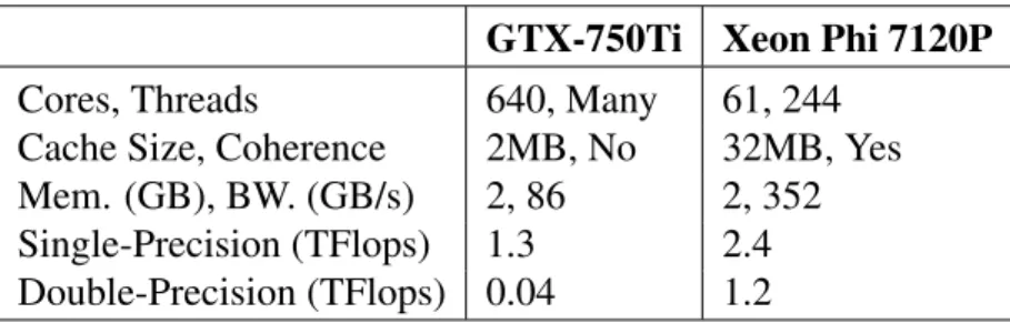
Two accelerators are primarily evaluated to build the multi-accelerator architecture, NVidia GTX-750TI and Intel Xeon Phi 7120P (parameters listed in Table6.2.1). These accelerators are competi-tive as their compute performance (single/double precision) overlap. Although the double precision capability of the Xeon Phi is higher, not all benchmark combinations require it during execution, and hence it contributes to the chip differences between accelerators which vary performance. The main memory used by both accelerators is pinned to the smallest one available. Memory size is not considered as a first-order effect in our work due to the fact that the whole architecture needs to be reconfigured and relearned for memory size changes. Still, a sensitivity study is done to show memory size effects, where the memories of both accelerators are swept and performance is acquired for all combinations. Storage to stand-alone memory transfer times are not measured, as they are assumed to be constant.
To evaluate with a more powerful GPU, we choose an NVidia GTX-970 to replace the smaller 35
36 Table 6.2.1: Primary Accelerator Configuration.
GTX-750Ti Xeon Phi 7120P
Cores, Threads 640, Many 61, 244 Cache Size, Coherence 2MB, No 32MB, Yes Mem. (GB), BW. (GB/s) 2, 86 2, 352 Single-Precision (TFlops) 1.3 2.4 Double-Precision (TFlops) 0.04 1.2
GPU for the multi-accelerator setup. GTX-970 incorporated 1664 cores with 3.5 TFLOPs single-precision and 0.1 TFLOPs double-single-precision compute capability, and has a larger 4 GB memory size. This work also evaluates an Intel Xeon E5-2650 v3 multicore having 10 hyper-threaded cores in 4 sockets, executing at 2.30GHz, with a 1TB DDR4 RAM. In addition to the primary (GTX-750TI, Xeon Phi) configuration, the following accelerator combinations are analyzed: (GTX-970, Xeon Phi), (GTX-750TI, CPU-40-Core), and (GTX-970, CPU-40-Core).
6.2
Benchmarks
For multicore benchmarks, SSSP-Bellman-Ford (SSSP-BF), BFS, DFS, PageRank, PageRank-DP, Triangle Counting (Tri.Cnt.), Community Detection (Comm.), and Connected Components (Conn. Comp.) are acquired from CRONO [8], MiBench [34], and Rodinia [35]. As SSSP-BF may not provide optimal performance on lower core counts in multicores, an SSSP implementation using
∆-Stepping (SSSP-Delta) is also acquired from the GAP benchmark suite [14] and compared. These versions use pthread/OpenMP implementations to run on multicores (using the offload programming model). For GPUs, benchmarks are acquired from Pannotia [5] and Rodinia [35] for OpenCL workloads, which provide SSSP, BFS, PageRank, and PageRank-DP. The remaining benchmarks are ported from the multicore implementations to OpenCL.