The Short-time Behavior of VIX Implied Volatilities in a
Multifactor Stochastic Volatility Framework
Andrea Barletta
∗Elisa Nicolato
†Stefano Pagliarani
‡This version: November 28, 2017
Abstract
We consider a modeling setup where the VIX index dynamics are explicitly computable as a smooth transformation of a purely diffusive, multidimensional Markov process. The framework is general enough to embed many popular stochastic volatility models. We develop closed-form expansions and sharp error bounds for VIX futures, options and implied volatilities. In particular, we derive exact asymptotic results for VIX implied volatilities, and their sensitivities, in the joint limit of short time-to-maturity and small log-moneyness. The obtained expansions are explicit, based on elementary functions and they neatly uncover how the VIX skew depends on the specific choice of the volatility and the vol-of-vol processes. Our results are based on perturbation techniques applied to the infinitesimal generator of the underlying process. This methodology has been previously adopted to derive approximations of equity (SPX) options. However, the generalizations needed to cover the case of VIX options are by no means straightforward as the dynamics of the underlying VIX futures are not explicitly known. To illustrate the accuracy of our technique, we provide numerical implementations for a selection of model specifications.
Keywords: VIX options, multifactor stochastic volatility, asymptotic expansions.
JEL Classification: C60; G12; G13.
1
Introduction
The CBOE’s volatility index (VIX index), first published in 1993 and revised in 2003, extrapolates market expectations of future volatility from a portfolio of listed options written on the S&P500 index (SPX index). The constituting portfolio, detailed in theCBOE(2009) white paper, is selected so that the VIX squared is an approximate replication of the fair swap rate of a 30-days realized variance swap. Thus, the VIX index can be seen as a model-free measure of the 30-days risk-neutral market volatility. Following the interest of market participants towards pure volatility trading instruments, VIX futures and VIX options were introduced in 2004 and 2006 respectively. Since then, the market of VIX derivatives has grown rapidly and now constitutes a quarter of the total turnover in derivatives on the SPX index.
∗Department of Economics and Business Economics, Aarhus University, Denmark.e-mail: [email protected]. †Department of Economics and Business Economics, Aarhus University, Denmark. e-mail: [email protected].
‡DIES, Universit`a di Udine, Udine, Italy.e-mail: [email protected]. This work was partially supported by the Chair
Clearly, there is a deep connection between the VIX index, the SPX index and the corresponding options and futures. De Marco and Henry-Labordere(2015) show that SPX options and VIX futures provide model independent bounds for VIX options via the resolution of a martingale optimal transportation problem. Further structural links are investigated by Papanicolaou (2014), who determines a model-free connection between the risk-neutral VIX tail distribution and the negative moments of the SPX index. Thus, the valuation of VIX derivatives requires a pricing model which should reproduce the stylized facts of both the SPX and the VIX option markets and match the corresponding implied volatility surfaces as close as possible. Several modeling approaches have been proposed in the literature. In the smile paper series,Bergomi
(2004,2005,2008,2009) develops a framework which builds upon the joint dynamics of the underlying spot and its implied forward variance swap curve. In the same spirit are the contributions ofBuehler(2006) and
Cont and Kokholm(2013), whileHuskaj and Nossman(2013) andBadran and Goldys(2015) directly spec-ify the term structure of VIX futures.Madan and Yor(2011) model the log-SPX as a Sato process running at a speed governed by the VIX level and Carr and Madan(2014) model the joint density of the VIX, the SPX and the realized variance at a fixed maturity.
A more traditional approach is to utilize a stochastic volatility (SV) structure, where the joint dynamics of the SPX price and its instantaneous variance are driven by a diffusion process, possibly multi-factor. Besides the celebrated Heston (1993) benchmark, popular one-factor SV models include the 3/2 model of
Heston (1997) (see alsoCarr and Sun(2007) and Drimus(2012a)), the continuous time GARCH model of
Lewis(2016) (see alsoChristoffersen et al.(2010)) and the solvable class ofItkin(2013). Within the multi-factor SV framework, we mention the double mean reverting model ofGatheral(2008), the double Heston model of Christoffersen et al. (2009), the 4/2 model of Grasselli (2016) and the recent Heston stochastic vol-of-vol model ofFouque and Saporito(2017).
As far as SPX options are concerned, many authors have contributed to the understanding of how the characteristics of a specific SV model impact the shape and the dynamics of the associated SPX implied volatility surface. A classical reference is the work ofLewis(2016) who derives asymptotic expansions both for the short and the long-dated limits under the assumption of small vol-of-vol. Analogous results are ob-tained bySircar and Papanicolaou(1999),Fouque et al.(2000),Lee(2005) under slow or fast mean-reversion regimes for the volatility process. More general SV models are considered in Berestycki et al. (2004) and
Durrleman(2010) who derive asymptotic formulae near expiry by studying the quasi-linear parabolic initial value problem defining the implied surface. Large deviation techniques have been employed by a number of authors as well. Here we mention Forde and Jacquier(2011), Forde et al.(2012),Caravenna and Corbetta
(2017),Deuschel et al.(2014a,b) andFriz et al. (2017) for the analysis of purely diffusive SV models, while
Jacquier et al.(2013) extend the large-deviation approach to SV models allowing for jumps. Jump-diffusions are also considered by Al`os et al.(2007) andBenhamou et al.(2009) who employ Malliavin calculus, while
Medvedev and Scaillet(2007) provide short-time implied volatility approximations by means of yet another method.
Particularly relevant for this work are the recent results obtained byPagliarani and Pascucci(2017) in a very general — albeit purely diffusive — multidimensional Markovian SV setup. These authors determine ex-plicit approximations for the implied volatilities, and their sensitivities, which asymptotically converge to the exact values within a parabolic region of the log-strike/time-to-maturity space. The methodology of choice combines perturbation theory with Dyson series to find approximate solutions of PDEs. This technique has been developed throughout a series of papers including Pagliarani and Pascucci(2012), Lorig et al.(2015),
Lorig et al.(2017) and Pagliarani and Pascucci(2017). For brevity, we aggregate all these contributions in a single reference, and we refer to the results therein as the results or the technique by LPP. However, we point out that similar results are obtained inBompis and Gobet(2013) andCaravenna and Corbetta(2016) by means of different approaches.
We stress that the entire body of literature surveyed above deals with the volatility surface implied by SPX options in models where the SPX index dynamics are exogenously specified. In this work, we assume that the pricing framework allows for explicit VIX index dynamics and we turn attention to the volatility surface implied by VIX options. Our main goal is to develop closed-form (polynomial) expansions which are consistent with the exact asymptotic behavior of the VIX implied volatility surface in the joint short time/small log-moneyness regime. As the VIX index is not a traded asset, VIX options should be seen as contracts written on the co-expiring VIX futures rather than the VIX index itself, and the VIX implied volatilities must be computed accordingly, via inversion of the Black (1976) formula. In particular, matu-rity-dependent features of the VIX volatility surface, such as the short time/small log-moneyness behavior, are naturally linked to the dynamics of the underlying futures prices. However, in many pricing models the VIX futures prices are not computable in closed-form even if the VIX index is.
In a recent paper, Fouque et al. (2014) address a similar issue. These authors consider the pricing of contracts written on the futures price of a non traded asset, such as the VIX, under the assumption that the spot dynamics are governed by a multiscale SV model. Under few additional assumptions on the futures pricing function, e.g., its invertibility with respect to the asset value, they derive first-order approximations for options and their implied volatilities.
The approach we adopt in this work is similar as we also assume that the dynamics of the VIX index are explicitly given. More precisely, we assume that the VIX index, here denoted by V, is determined via a smooth transformation (Vt=φ(Yt, t))t≥0 of a purely diffusive and possibly multidimensional Markov
processY. While we assume that the functionφis computable in closed form, we do not impose any further structural restriction onφ, the factorsY or the pricing function for futures prices. This framework is flexible enough to encompass all the classical SV models mentioned above as well as models in the spirit of those proposed byBergomi(2005,2008). Furthermore, it includes some SV models allowing for jumps in the SPX price process such as the augmented 3/2 model of Baldeaux and Badran (2014) and many specifications within the time change L´evy framework of Carr et al. (2003). As we shall see, being able to handle such a general framework comes with a price; namely the necessity of artificially raising the dimension of the underlying Markovian dynamics, thus leading to a fully degenerate diffusion.
In this setup, we develop explicit approximations and sharp error bounds for VIX futures and VIX option prices. More importantly, we derive closed-form expansions for VIX implied volatilities, and their sensitivi-ties, which are asymptotically exact in the joint limit of short time-to-maturity and small log-moneyness. We achieve these results by performing adouble-layer version of the above mentioned technique by LPP which allows us to bypass the lack of explicit VIX futures dynamics. We first apply the technique to the known VIX index dynamics in order to obtain approximate VIX futures prices. We also determine short-time error bounds for the approximation and its derivatives. Next we apply the technique to theunknownfutures prices dynamics to compute approximate VIX option prices. These, in whole generality, are also unknown. However, by combining the asymptotic results of the first layer with a suitable centering of the expansions we can attain option prices approximations which are explicit. Finally, we apply the LPP conversion to transform the approximate prices into explicit implied volatilities which are then proven to be asymptotically exact.
We point out that the double-layer procedure is primarily instrumental to the approximation of the volatility surface and its asymptotic analysis. Had we been concerned uniquely with the pricing of VIX futures and VIX options, we could have applied the technique by LPP directly to the VIX index dynamics to obtain prices relative to the VIX spot value. Instead, we employ the double-layer methodology to price options relatively to the futures prices dynamics. This is required by the above mentioned technique to ob-tain approximations for implied volatilities and their sensitivities which are polynomial and asymptotically convergent to the exact values.
The double-layer procedure sketched above hides a number of subtle difficulties. In the original version of the technique by LPP, the error bounds are determined under some ellipticity assumption for the involved operators. In the setup of the present work, we are forced to deal with fully degenerate generators partly to allow for computations in closed-form, and partly to comply with the structural requirements of the methodology. We overcome this difficulty by employing a regularization technique which is known in PDEs theory, and that was recently applied by Leung et al. (2017) to study leveraged ETF implied volatilities: It consists in introducing a small perturbation along an extra diffusion component and then passing to the limit. It is also important to highlight that to obtain asymptotic results for VIX implied volatilities, we must operate in a joint regime of time-to-maturity and log-strike: the underlying values of the VIX futures prices depend on maturity and therefore the log-strike of an ATM VIX-call approaches the spot value along a curve which is not a straight line as the time-to-maturity shrinks to zero. Thus, the vertical limits at fixed log-strike derived e.g., in Berestycki et al. (2004) and Durrleman(2010) do not apply to the setting of this work. Luckily, the recent results by Pagliarani and Pascucci(2017) naturally adapt to our case and allow us to compute expansions around the spot value of the VIX index which asymptotically yield the exact value. The main result concerning our double-layer approximation is given in Theorem 3.10, where we provide the sharp error bounds within the parabolic region relevant for the VIX implied volatilities. The exact asymptotic values are then computed in Corollary3.11.
The rest of the paper proceeds as follows: in Section 2 we introduce the modeling assumptions for the dynamics of the VIX index, and we discuss a number of popular pricing models embedded in our framework. In Section 3 we provide a full description of the double-layer approximating technique that we design to obtain asymptotic expansions for VIX implied volatilities, in a joint region of short time-to-maturity and small log-moneyness. In Section 4 we provide numerical examples to test the accuracy of our approximate formulas for a variety of model specifications. In Section5 we conclude. In the Appendix, we describe the main features of the technique by LPP, we provide the proofs of our results, and we explicitly report some general formulae for the implied volatility expansions obtained in Section 3. MATLAB and Mathematica codes to compute these formulae are publicly available at https://abarletta.github.io/viximpv/and
https://explicitsolutions.wordpress.com, respectively.
2
The modeling framework
We consider a frictionless market model living on a filtered probability space Ω,F,(Ft)t≥0,Q
which satisfies the usual conditions. Without loss of generality, we consider a normalized economy with zero interest rates and dividend payments, and we assume that Q is the risk-neutral measure adopted for all pricing purposes. By the no arbitrage hypothesis, the price S of the underlying SPX index follows a Q -martingale which we assume to be strictly positive. Following theCBOE(2009) white paper, the portfolio
defining the square of the VIX index statically replicates a log-contract expiring 30 days ahead. Maintaining the notation anticipated in the introduction, the VIX squareV2is then defined as follows
Vt2:=− 2 ∆E log St +∆ St Ft , t≥0, (2.1)
where the time lag is fixed at ∆ = 30/365, and Edenotes the expectation underQ.
The central modeling hypothesis of this work is that the VIX process V is determined by a smooth transformation of a finite dimensional Markov process with diffusive dynamics. More precisely, we assume the following.
Assumption 2.1. The VIX processV takes the form
Vt:=φ(t, Yt), (2.2)
where φis a smooth, positive-valued functionφ(·,·) :R≥0×Rd →R≥0, andY is ad-dimensional Markov
process taking value on a domainDY ⊆Rd, with risk-neutral dynamics
dYt=αY(t, Yt)dt+ηY(t, Yt)dWt, t >0, (2.3) whereW denotes ad-dimensional Brownian motion. The functionφis assumed to be computable in closed-form.
Many popular pricing models comply with Assumption 2.1. Consider, for example, the time-changed L´evy framework proposed byCarr et al.(2003). Here, the log-price process is obtained by evaluating a L´evy processL, withE[eL1]<∞, at an absolutely continuous random clock
logSt:=LRt
0τsds,
whereτis a positive stochastic process representing the instantaneous rate of time change. Let (βL, γL, ϕL(dx))
denote the L´evy triplet of the subordinand L´evy processLwith respect to the identity function. By Lemma 5 inKallsen and Shiryaev(2002), the log-price dynamics admit the following representation
d logSt=βLτtdt+pγLτtdBt+ dJt, (2.4)
where B is a Brownian motion, J is a pure-jump, zero-mean martingale process with jump compensator
νJ(dx, dt) =ϕL(dx)τtdt, and βL is constrained to be βL=− 1 2γ L+Z R0 (ex−1−x)ϕL(dx) (2.5) by the martingale property of S. In this modeling framework, the expression (2.1) for the VIX square becomes Vt2=− 2βL ∆ E " Z t+∆ t τsds Ft # .
Next, we briefly recall a number of random clock specifications for which the VIX fulfills the requirements of Assumption2.1.
TheHeston(1993) model, as well as the purely jumping NIGSV and VGSV models proposed byCarr et al.
(2003), build upon the CIR random clock by setting
dYt=λ(θ−Yt) dt+ǫpYtdWt, (2.6) whereλ,θandǫare positive constants. As the drift is affine in the state variableY, it is immediate to verify that the VIX index is given by
Vt2=− 2βL ∆ (aYt+b), (2.7) wherea= 1 λ 1−e− λ∆
,b=θ(∆−a) and ∆ is the 30 days time-lag.
Another well known specification is the so-called 3/2 model proposed by Lewis (2016), and recently reprised byDrimus(2012a) andBaldeaux and Badran(2014) among others. The stochastic clock is set to
τt=Yt
dYt=λYt(θ−Yt) dt+ǫYt3/2dWt,
whereλ,θand ǫare positive constants. In this case, the VIX formula reads as follows
Vt2=− 2βL ∆ h Yte ∆λθ−1 λθ , (2.8) where h(x) = Z x 0 e−ǫ22z z 2λ ǫ2 Z ∞ z 2 ǫ2e 2 ǫ2u u− 2λ ǫ2−2du dz .
For the derivations, we refer to Theorem 4 inCarr and Sun (2007) where also the case of time-dependent coefficients is covered.
A simple application of Itˆo’s Lemma shows that whenY follows the CIR dynamics (2.6) under the Feller condition 2λθ > ǫ2, the process 1/Y displays dynamics of the 3/2 type (2.8). Based on this observation,
Grasselli(2016) constructs the4/2 model by setting
τt=α2Yt+β2 1 Yt+ 2αβ
whereα,βare real constants andY is given in (2.6). The VIX squareV2is then given by the corresponding
affine combination of expressions (2.7) and (2.8), albeit re-parametrized.
Further solvable one-factor models are discussed in Itkin (2013), who considers random clocks of the following type τt=Yt2 dYt=q(t)Ytα−s(t)Y β t dt+p(t)Ytγ+1dWt,
where α, β, γ ∈ R, while q(·), s(·), and p(·) are deterministic functions of t. The author employs Lie symmetries techniques and, for several concrete specifications, determines explicit VIX formulas in terms of hypergeometric functions.
Another popular specification is the so-calledexponential Ornstein-Uhlenbeck model first introduced by
Scott (1987) and further analyzed by Masoliver and Perell´o(2006), Perell´o et al. (2008) and Sepp(2016) among others. A detailed discussion of this model specification is postponed to Section4.
As for multi-factor models, many specifications share affine-drift dynamics of the following type
τt=ωYt
whereW is a d-dimensional Brownian motion,A∈d×dmatrix,B ∈Rd , andηY is ad×dmatrix-valued
function. The factorsY = (Y1, . . . , Yd)⊤ are loaded into the random clock via the (row) vectorω∈Rd. In
this case, the VIX square is an affine transformation of the factors
Vt2=aYt+b (2.9) where a = −2∆βL R∆ 0 ωeAsds and b = − 2βL ∆ R∆ 0 Rs
0 ωeAuB du ds. The double mean-reverting model of
Gatheral (2008), the double Heston model of Christoffersen et al. (2009) and the stochastic volatility of volatility model are embedded in this framework and will be further analyzed in Section4.
3
Approximating VIX futures, options and implied volatilities
Recall that we work in a zero interest rates economy governed by a risk-neutral measure. Thus, the price at timet≥0 of a VIX call with strikeek,k∈R, and expiryT ≥t, here denoted bycvix
t,T,k, is given by cvix
t,T,k=E[ VT−ek
+
|Ft]. (3.1)
Since the VIX index is not a traded asset relations such as put-call parity and calculations of hedge ratios presume that the underlying asset is in fact the futures price of the VIX with expiry set at maturity T, which is
FtT =E[VT|Ft], 0≤t≤T . (3.2)
While the spot and the futures VIX coincide at maturityT, i.e.,FT
T =VT, the two quantities typically differ
for t < T, as the VIX index V is not necessarily a martingale. In particular, VIX implied volatilities are defined as follows.
Definition 3.1. For any k ∈ R and 0 ≤ t < T, the VIX implied volatility (VIX-IV, for short) σimpt,T,k is defined as the unique positive solution of
cvix
t,T,k=uBS σimpt,T,k; logFtT, k, T −t
, (3.3)
whereFT
t is VIX futures price defined in (3.2), anduBS is theBlack(1976) call price function, i.e. uBS(σ;x, k, τ) := exN(d+)−ekN(d−), d± := 1 σ√τ x−k±σ 2τ 2 , (3.4)
whereNis the CDF of a standard normal random variable.
The objective of this section is to derive closed-form expansions for VIX implied volatilities, and their sensitivities, which are asymptotically exact in the joint limit of short time-to-maturity and small log-mon-eyness. As mentioned in the Introduction, we plan to employ the technique by LPP and extend the results obtained for SPX implied volatilities to the VIX volatility surface. The general approximating methodology is detailed in Appendix A.1. In particular, the explicit approximation of implied volatilities is carried out in Appendix A.1.2 and it stipulates that option prices are to be approximated by expanding the log-prices dynamics of the underlying asset, which, in light of Definition 3.1, appears to be the VIX log-futures price. Bearing that in mind, letAYt denote the generator of the Markov processY satisfying (2.3) in Assumption
2.1, i.e., AYt =AYt(y) =1 2 d X i,j=1 aYij(t, y)∂yiyj+ d X i=1 aYi (t, y)∂yi, (t, y)∈R≥0×DY (3.5)
where aYij = ηY(ηY)⊤ ij, and a Y i =αYi , for i, j= 1,· · ·, d. (3.6)
Also recall that DY ⊆Rd denotes the domain ofY. Then, under mild regularity conditions (see Assump-tions3.3–3.4and Remark3.5below), the VIX futures priceFT
t can be written as FtT =E
φ(T;YT)|Yt
=f(t, Yt;T), 0≤t≤T ,
with the functionf(·,·;T) satisfying the backward problem
∂t+AYt f(t, y;T) = 0, on [0, T[×DY, f(T, y;T) =φ(T, y), y∈DY. (3.7)
With the functionf at hand, we can employ Itˆo’s formula to derive the dynamics of the underlying log-VIX futures prices
XtT = log(FtT), 0≤t≤T .
They read as follows
dXT t =− 1 2 ηT(t, Yt) 2 dt+ηT(t, Yt)dWt, 0< t≤T , (3.8)
where the functionηT(·,·) : [0, T]×DY →Rd is given by ηT(t, y) = ∇yf(t, y;T)
ηY(t, y)
f(t, y;T) . (3.9)
So, our goal is to approximate the implied volatilities of calls written on the (log-) futures component of the (d+ 1)-dimensional Markov processZT = (Y, XT) with generatorAT
t given by ATt =ATt(y) =1 2 d+1 X i,j=1 aTij(t, y)∂zizj + d+1 X i=1 aTi(t, y)∂zi, (t, y)∈R≥0×DY, (3.10) where aTd+1i=aTi d+1= ηT(ηY)⊤ i, a T ij = ηY(ηY)⊤ ij, a T i =αYi , i, j= 1,· · ·, d, (3.11) and aT d+1d+1=|ηT 2 , aT d+1=− 1 2|η T 2 , (3.12)
with αY, ηY given in (2.3) and ηT defined in (3.9). Note that, although AT
t is a differential operator on
Rd+1, its coefficients only depend on the firstdvariables, i.e. ony ∈DY. Also, the VIX call price in (3.1)
can be written as cvixt,T,k=E eXTT −ek+|ZT t =u t, Yt, XtT;T, k , 0≤t≤T, k∈R, (3.13) and the implied volatility in (3.3) can be written as
σt,T,kimp =σ t, Yt, XtT;T, k
. (3.14)
At first glance, this seems to be the appropriate setting to approximate — and subsequently analyze — the VIX implied volatility surface via the LPP methodology: Based on an expansion of the generatorAT t
given in (3.10), the call price functionuand the implied volatility functionσare approximated according to DefinitionsA.2andA.4respectively. A closer inspection of expression (3.10), however, clarifies that a direct application of the results by LPP to the modeling framework of this work is not feasible. The obstacles we need to face are the following:
• First, the generatorAT
t is typically unknown: from (3.11)–(3.12) we see that the coefficients depend
on the futures price function f, i.e., the solution of (3.7), which in most model specifications cannot be computed explicitly.
• Second, the generator AT
t is fully degenerate, i.e., the diffusion matrix of the processZT = (Y, XT)
is singular at any point as XT
t is a deterministic transformation of Yt. Under further assumptions
on the function f, such as invertibility w.r.t. one ore more variables, it could be possible to obtain a d-dimensional, non degenerate Markov process ˜ZT = (XT,Y˜), with ˜Y being a (d−1)-dimensional projection of Y. However, this approach would narrow the range of application of our method and the procedure would be more complicated and less elegant. In fact, as pointed out in Remark A.3, the construction of the approximations is not at all affected by the singularity of ZT = (Y, XT).
However, the asymptotic results available from previous works do not apply as they strongly rely on the assumption of local ellipticity for the generator. See, e.g., the recent paper byPagliarani and Pascucci
(2017).
To deal with the first issue, we propose adouble-layer version of the approach by LPP which can be sketched as follows:
Step 1 Based on the known generator AYt of the VIX factorsY, we apply a first layer expansion to derive theN-th order approximation ¯fN(¯t,y¯)of the futures price functionf. Here, we also determine the short
time-to-maturity asymptotic error bounds of the approximation and its derivatives.
Step 2 Based on the unknown generator ATt, we apply a second layer expansion to derive the N-th order approximation ¯uN(¯t,¯y) of the call price function u, which, a priori, is also unknown. However, the asymptotic analysis of step 1 reveals that when setting ¯t =T the approximation ¯u(NT,y¯) is explicitly
computable.
Step 3 Based on ¯uN(T,y¯), we compute the implied volatility expansions ¯σN(T,y¯) in accordance to DefinitionA.4. Finally, evaluating ¯σ(NT,y¯) at ¯f
(T,y¯)
M and choosing the order M and the point ¯y suitably, we obtain
ap-proximations which, in the joint limit of short maturity and small moneyness, converge asymptotically to the exact value.
As for the second issue, we deal with fully degenerate operators by employing the PDE regularization technique briefly mentioned in the Introduction. The detailed explanation is delayed to AppendixA.2where such regularization is needed to analyze error bounds for the approximations ¯fN(¯t,y¯), ¯uN(¯t,y¯) and ¯σN(¯t,y¯).
An important remark is now in place.
Remark 3.2. We emphasize that the double-layer approach is designed specifically to approximate and an-alyze VIXimplied volatilities rather than VIXoption prices. Had the pricing problem been the main focus, we could have employed a direct version of the LPP technique in various ways. For example, we could have expanded the known generator AY
t of the factors process Y to price the payoff function (φ(T, YT)−ek)+.
Alternatively, we could also have expanded the known generator of the pair (Y, V) and price VIX options relatively to the VIX index value. However, these direct approaches yield option prices in a form which is not suitable for the LPP conversion to implied volatilities expansions, as this construction requires price expansions based on the generator of the pair (Y, XT). See AppendixA.1.2 for details.
Before proceeding to implement the three steps outlined above, we state the regularity conditions which the factorsY must satisfy for the validity of our analysis. Throughout the rest of this section we fixN∈N0
T0>0, and we enforce the following assumptions.
Assumption 3.3. The generator of Y, i.e. AYt as in (3.5)-(3.6), is such that, for any finite subdomain
D′
Y ⊂DY there exists M >0 for which the following properties hold:
(i) Regularity and boundedness: the coefficientsaY
ij, aYi ∈CPN+1([0, T0[×DY) with partial derivatives up
to orderN+ 1 bounded byM on [0, T0[×D′Y. HereC N+1
P denotes the usual parabolic space of order N+ 1, i.e. the space of functions with derivatives up to theN+ 1-th order, where one derivative in t
compares to two derivatives iny (see, for instance, Chapter 10.1 in Friedman(1976)). (ii) Local ellipticity:
M−1|ζ|2≤ d X i,j=1 aY ij(t, y)ζiζj≤M|ζ|2, t∈[0, T0[, y∈D′Y, ζ∈Rd.
Assumption 3.4. The processY is a Feller diffusion on [0, T0[×DY, i.e. for anyT ∈]0, T0[ andϕ∈Cb(Rd)
the function (t, y)7→Et,y[ϕ(YT)] is continuous on [0, T[×DY.
We conclude with a final observation which, for ease of reference, we state in the following Remark.
Remark 3.5. Under Assumptions2.1,3.3and 3.4the futures prices functionf does satisfy the backward problem (3.7) and it is of class CPN+2([0, T]×DY). For a proof see e.g., Theorem 2.3 and Remark 4.3 in
Pagliarani and Pascucci(2017).
3.1
First step: VIX futures expansions
We start by developing the expansion for the futures price function f. In view of Remark 3.5 it may seem natural to approximatef by applying the technique by LPP directly to the backward problem (3.7). However, as pointed out in RemarkA.3-(ii), the corresponding expansion is computable in closed form only if the integral ofφ(·, T) against a Gaussian density is computable in closed form. As this is typically not feasible, we adopt a different strategy. First we compute the dynamics of of the VIX processV. By applying Itˆo’s formula to (2.2) we obtain
dVt=µV(t, Yt)dt+ηV(t, Yt) dWt, t >0, (3.15) with µV(t, y) = ∂t+AYt(y) φ(t, y) = ∂tφ+1 2 d X i,j=1 ηY(ηY)⊤ ij∂yiyjφ+ d X i=1 µYi (∂yiφ) (t, y), (3.16) ηV(t, y) =∇yφ(t, y)ηY(t, y), (3.17)
for any t ∈ [0, T0[ and y ∈ DY. Next we consider the Rd+1-valued Markov process Z := (Y, V) with
generatorAtgiven by At=At(y) =1 2 d+1 X i,j=1 aij(t, y)∂zizj + d+1 X i=1 ai(t, y)∂zi, (t, y)∈R≥0×DY , (3.18)
where ad+1i =ai d+1= ηV(ηY)⊤ i, aij = η Y(ηY)⊤ ij, ai=µ Y i , i, j= 1,· · ·, d, and ad+1d+1=ηV ηV⊤, ad+1=µV.
HereµV andηV are as in (3.16)-(3.17). Finally, we re-write the VIX futures price as follows
FtT =E[VT|Zt] =g(t, Yt, Vt;T), 0≤t≤T . (3.19)
The coefficients ofAtdepend uniquely on theycomponent of the variablez= (y, v) and therefore they fulfill, in view of Assumption3.3-(i), the regularity required by AssumptionA.1on the domain [0, T0[×DY×R. We
can then expandAtaround a point (¯t,y¯) to construct theN-th order approximation ¯g(¯t,y¯)
N of the functiong
according to DefinitionA.2. As the final datum in (3.19) is trivially integrable against a univariate Gaussian density, the terms of ¯gN(¯t,y¯) are explicitly computable. The zero order term, given in (A.8), becomes the following affine transformation of (T−t)
g0(¯t,y¯)(t, y, v;T) =v+ (T−t)ad+1(¯t,y¯) =v+ (T−t)µV(¯t,y¯).
The higher order terms gn(¯t,y¯)(t, z;T), given in (A.9), are polynomial functions of (T −t) and (yi−yi¯). At
the first order we have
g1(¯t,y¯)(t, y, v;T) = Z T t G1(¯t,y¯)(t, s, y, v)g0(¯t,y¯)(t, y, v;T)ds = Z T t d X j=1 ∂yjad+1(¯t,y¯) yj−yj¯ + (s−t)aYj(¯t,y¯) ds = (T −t) d X j=1 ∂yjµ V(¯t,y¯) yj−yj¯ +(T −t) 2 µ Y j(¯t,y¯) .
for any (¯t,¯y) ∈[0, T]×DY. The remaining higher order terms can be explicitly computed by means of a symbolic computation software. Finally, we recall that the futures pricing functionf is recovered fromg via the relation
f(t, y;T) =g t, y, φ(t, y);T
, (3.20)
and we define theN-th order approximation ¯fN(¯t,y¯)as follows
f(t, y;T)≈f¯N(¯t,y¯)(t, y;T) := ¯g(¯Nt,y¯) t, y, φ(t, y);T
. (3.21)
So fromg0(¯t,y¯),g(¯1t,y¯) above we obtain
f0(¯t,y¯)(t, y;T) =φ(t, y) + (T−t)µV(¯t,y¯) and f (¯t,y¯)
1 (t, y;T) =g (¯t,y¯)
1 (t, y, v;T), (3.22)
as g(¯1t,y¯) does not depend onv. The choice of the point (¯t,y¯)∈[0, T]×DY is somehow arbitrary. However,
for the particular choices (¯t,y¯) = (T, y) and (¯t,y¯) = (t, y), we are in the position to provide sharp error bounds for the approximate futures price function ¯fN(¯t,y¯)and its sensitivities.
Theorem 3.6. Let Assumptions 2.1,3.3 and 3.4 be in force. Then, for any finite subdomain D′
Y ⊂DY, t∈[0, T0[, and for anyq∈N0,β∈Nd0 with2q+|β| ≤N+ 2, we have:
∂ q tDyβf(t, y;T)−∂ q tDβyf¯ (¯t,y¯) N (t, y;T)|¯t=T,y¯=y =O (T −t)N−|β|−22q+3 , and ∂ q tDβyf(t, y;T)−∂ q tDyβf¯ (¯t,¯y) N (t, y;T)|¯t=t,y¯=y =O T −tN−|β|− 2q+3 2 ,
asT →t+, uniformly w.r.t. y∈DY. Here we have employed the multi-index notation explained in (A.5).
We postpone the proof of Theorem3.6 to Appendix A.2and we conclude this section with a couple of observations.
Remark 3.7. (i) We point out that we construct ¯fN(¯t,y¯)by Taylor-expanding the coefficientsaij,ai both
along the space y and the time t variables. This is in contrast to how the technique by LPP is applied in previous papers, where only expansions in the space dimension are employed. Although our choice introduces an additional error in the approximate solutions, it allows to obtain explicitly computable approximations also in the case of time-dependent coefficients. Furthermore, we choose the parabolic Taylor series as opposed to the classical Taylor series as the former has the right homogeneity needed to perform the error analysis in the case that (∂t+A) is a parabolic operator. More precisely, the parabolic Taylor expansion is computationally the cheapest polynomial expansion yielding an approximating series that is asymptotically convergent for short times. This follows from the known fact that a parabolic operator is homogeneous of degree two w.r.t. to the dilations (t, z)7→(ℓ2t, ℓz),
ℓ >0.
(ii) Under the assumption of locally elliptic operators, error bounds similar to those stated in Theorem3.6
have been determined byPagliarani and Pascucci(2017). However, such results are not directly appli-cable to ¯fN(¯t,¯y)that builds upon generatorAt, which is fully degenerate.
3.2
Second step: VIX call prices expansions
We now proceed to construct approximations for the VIX call pricing function u= u(t, y, x;T, k) defined by (3.13). We have already observed that the generatorATt of the underlying process (Y, XT) is not
nec-essarily known. Still, from expressions (3.10)-(3.12) combined with Remark3.5we see that the coefficients
aT
i, aTij satisfy AssumptionA.1on the domain [0, T]×DY ×Rand therefore theN-th order approximation
¯
u(¯Nt,y¯)(t, y, x;T, k) is well defined for any fixed (¯t,y¯) ∈ [0, T]×DY. Once again the expansion is centered around (¯t,y¯) as the coefficientsaT
i, aTij only depend on theycomponent of the variable (y, x). In accordance
with (A.8), the zero order term is given by
u(¯0t,y¯)(t, y, x;T, k) =uBS σ(¯0t,y¯);T−t, x, k
, with σ0(¯t,y¯)=qaT
d+1d+1(¯t,y¯), (3.23)
while the remaining correcting termsu(¯nt,y¯)are given in (A.9). For instance, at order 1 we obtain
u(¯1t,y¯)(t, y, x;T, k) = Z T t G(¯1t,¯y)(t, s, y, x)uBS σ0(¯t,y¯);T−t, x, k ds= =(T−t) 2 hXd j=1 ∂yja T d+1d+1(¯t,y¯) yj−yj¯ +(T −t) 2 a T j(¯t,y¯) +aTj d+1(¯t,y¯)∂x i × (3.24)
× ∂xx−∂x
uBS σ(¯0t,y¯);T−t, x, k
,
and we delegate the computation of higher order terms to a symbolic computation software. Note that to obtain an explicitN-th order approximation ¯u(¯Nt,¯y)one must be able to compute the derivatives∂
q
tDβzaTij(¯t,y¯), ∂tqDβzaTi(¯t,y¯) with 2q+|β| ≤N, which in turn depend on the derivatives∂
q
tDβyf(¯t,y¯;T) with 2q+|β| ≤N+1.
For an arbitrary time point ¯tthis is not feasible, but for the specific choice ¯t=Tsuch derivatives are provided by an immediate corollary to Theorem3.6.
Corollary 3.8. Let Assumptions 2.1, 3.3 and 3.4 be in force. For any q ∈ N0, and β ∈ Nβ0 such that
2q+|β| ≤N+ 1, we have ∂tqDβ yf(t, y;T) t=T =∂ q tDβyf¯ (¯t,y¯) M (t, y;T) ¯ t=t=T,y¯=y, T ∈[0, T0[, y∈DY, (3.25)
where2q+|β| −2≤M ≤N andf¯M(¯t,¯y) is the approximation defined in(3.21). Above we set by convention
¯ f−(¯t,1y¯)= ¯f (¯t,y¯) −2 = ¯f (¯t,y¯) 0 .
Since the right-hand side of (3.25) is explicitly computable, Corollary3.8provides a way to compute the derivatives∂tqDβ
yf(t, y;T)|t=T. For instance, by using the 1-st order approximation ¯f1(¯t,¯y)we can recover all
the derivatives∂tqDβyf(t, y;T)|t=T with 2q+|β| ≤3, and thus all the derivatives∂tqDβyaTij(t, y),∂ q
tDβyaTi(t, y)
with 2q+|β| ≤ 2, which are needed to compute explicitly the 2-nd order approximation ¯u(2T,y¯). From
expression (3.22) combined with (3.25) we obtain the derivatives
Dβyf(t, y;T)|t=T =Dβyφ(T, y), |β| ≤3
and
∂tf(t, y;T)|t=T =∂tφ(T, y)−µV(T, y), ∂t∂yif(t, y;T)|t=T =∂t∂yiφ(T, y)−∂yiµ
V(T, y), i= 1,
· · ·, d.
So, the first two explicit termsu(0T,y¯)andu (T,y¯)
1 are obtained by inserting into (3.23) and (3.24) the following
expressions aTd+1d+1(T,y¯) = ∇yφηY 2 φ (T,¯y), a T j(T,y¯) =αYj (T,y¯), aTj d+1(T,y¯) = (∇yφ)ηY(ηY)⊤j φ (T,y¯). (3.26)
Remark 3.9. Similar to the futures prices approximation ¯fN(¯t,y¯), we derive the call approximation ¯u(¯Nt,y¯)by expanding the relevant generator coefficients not only in space, but also in time. As discussed in Remark3.7, for futures prices this is a somewhat optional choice mainly motivated by numerical convenience. In contrast, when dealing with call prices the choice to expand the unknown coefficients aT
ij(t,·), aTi (t,·) in both time
and space is mandatory, in order to obtain an explicit approximation by setting ¯t=T.
3.3
Third step: VIX implied volatility expansions
Let us recall that for a given call expansion ¯u(¯Nt,y¯), the corresponding implied volatility expansion ¯σ
(¯t,y¯)
N is
by evaluating the function σ t, y, x;T, k
at the log-futures pricex= logf(t, y;T). Therefore, we combine the first layer ¯fM(¯t,y¯)with the second layer ¯σN(¯t,y¯),M ≤N and approximate the true quantity as follows
σimpt,T,k≈σN(¯t,¯y) t, y,logfM(¯t,y¯)(t, y;T);T, k
. (3.27)
As discussed in Section3.2, the choice of the starting time is constrained to be ¯t=T so ¯u(NT,y¯)and therefore ¯
σN(T,y¯) is explicitly computable. Setting the starting spatial point ¯y =y and choosing a suitable order M
lead to approximations satisfying the following asymptotic error bounds.
Theorem 3.10. Let Assumptions 2.1,3.3and 3.4be in force. Then, for any finite subdomain D′
Y ⊂DY, t∈[0, T0[, and for anyℓ >0, it holds that:
σ t, y,logf(t, y;T);T, k
−σ¯N(T,y) t, y,log ¯fM(T,y)(t, y;T);T, k
=O (T−t)N+12 , (3.28) withN −2≤M ≤N, and ∂kσ t, y,logf(t, y;T);T, k
−∂k¯σN(T,y) t, y,log ¯fM(T,y)(t, y;T);T, k
=O
(T−t)N2
, (3.29) withN −3≤M ≤N, as(T, k)→(t,logv)within the parabolic region
Pℓ:= (T, k) |logv−k| ≤ℓ √ T−t , where v=φ(t, y), (3.30) uniformly w.r.t. y∈D′ Y. In(3.28)-(3.29), we set by convention f¯ (T,y)
n = ¯f0(T,y) for anyn <0.
The proof of Theorem3.10is postponed to AppendixA.2. An immediate application of this result yields the exact limit of the VIX implied volatilityσand its skewness∂kσas the time to maturity (T−t) shrinks and the log-strikekapproaches the current log-VIX value logφ(t, y) within the – arbitrarily large – parabolic regionPℓ defined in (3.30). In fact, both limits can be retrieved from the first order approximation ¯σ1(T,y)
evaluated at the zero order ¯f0(T,y). Combining DefinitionA.4with expressions (3.26) and (3.23), (3.24), we
obtain ¯σ(1T,y)=σ (T,y) 0 +σ (T,y) 1 with σ(0T,y)= ∇yφ(T, y)ηY(T, y) p φ(T, y) and σ(1T,y)(t, y, x;T, k) = u(1T,y)(t, y, x;T, k) ∂σuBS σ(T,y) 0 ;T−t, x, k = u(1T,y)(t, y, x;T, k) σ0(T,y)(T−t) ∂xx−∂x uBS σ(T,y) 0 ;T−t, x, k = (T −t) 4σ(0T,y) ∇y ∇yφ ηY 2 φ , α Y + ∇yφ ηY(ηY)⊤ 2φ (T, y) − (x−k) 4 σ(0T,y) 3 ∇y ∇yφ ηY 2 φ , ∇yφ ηY(ηY)⊤ φ (T, y),
where h·,·idenotes the scalar product of two vectors. The zero order futures price ¯f0(T,y)is given in (3.22)
and inserting it in the expression above leads to the following result.
Corollary 3.11. Under the assumptions of Theorem3.10, it holds that lim (T,k)→(t,logφ(t,y)) |logφ(t,y)−k|≤ℓ√T−t σ t,logf(t, y;T), y;T, k = ∇yφ(t, y) ηY(t, y) p φ(t, y) ,
and lim (T,k)→(t,logφ(t,y)) |logφ(t,y)−k|≤ℓ√T−t ∂kσ t,logf(t, y;T), y;T, k = ∇y ∇yφ ηY 2 φ , ∇yφ ηY(ηY)⊤ φ (t, y) 4 σ0(t,y) 3 , (3.31) for any (t, y)∈[0, T0[×DY.
Under few additional assumptions on the law ofY, it is possible to extend the results above to all the sensitivities∂Tq∂m
k σ, 2q+m≤N, and show that ∂ q T∂ m k σ t, y,logf(t, y;T);T, k −∂Tq∂km¯σ (T,y) N t, y,log ¯f (T,y) N−2−2q−m(t, y;T);T, k =O (T−t)N+1−22q−m (3.32) as (T, k)→ (t,logφ(t, y)) within Pℓ. Based on these error bounds, one can obtain the exact limits of the
derivatives at the initial point (t,logv) and e.g., carry out the exact Taylor formula of VIX implied volatility at a given order, thus extending the results in Pagliarani and Pascucci(2017) for SPX implied volatilities. This generalization, however, entails a lengthy analysis of rather technical nature. Therefore we do not specify further the assumptions ensuring the validity of (3.32), which is left without proof, and we refer the reader toPagliarani and Pascucci(2017) for further details.
4
Numerical illustrations for concrete specifications
In this section, we illustrate the accuracy of the VIX implied volatility approximation (3.27) under different SV models selected from the time-change framework described in Section2. For the sake of simplicity, we consider continuous dynamics for the log-price process, i.e., in expression (2.4) we set J = 0,γL = 1 and,
in view of (2.5), βL = −1/2. As for the stochastic clock — which here coincides with the instantaneous
variance — we consider the following popular specifications: • The mean-reverting CEV model ;
• The stochastic volatility of volatility model; • The double mean reverting model;
• The double Heston model;
• The exponential Ornstein-Uhlenbeck model.
In the first four cases, the VIX square takes the affine form given in (2.9). In the exponential Ornstein-Uh-lenbeck model, the VIX index cannot be expressed in term of elementary functions, but it can be computed via a simple numerical integration.
In each of these models we implement the double-layer approximation (3.27) with ¯y = y, ¯t = T and
M =N, withN up to the fourth order. To ease notation, we denote this approximation by ¯σN N, i.e., ¯
σN N(t, y;T, k) = ¯σ(NT,y) t, y,logfN(T,y)(t, y;T);T, k
. (4.1)
Some general formulae for the explicit expansions can be found in Appendix A.3. More precisely, we report expansions up to the order ¯σ22 for a general, albeit time homogeneous, one factor model, while
we stop at the order ¯σ11 for a two factors model which is general enough to embed the specifications
listed above. Higher-order approximations would take up too much space and thus are omitted. How-ever, approximations up to ¯σ44 can be computed using the codes provided in the authors’ web pages
https://abarletta.github.io/viximpv/andhttps://explicitsolutions.wordpress.com, implemented inMATLAB andWolfram Mathematica, respectively.
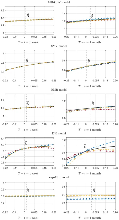
In virtue of Theorem3.10, we expect that ¯σN N is most accurate for close-to-expiry options with strikes nearby the initial VIX value. Therefore, we consider time-to-maturities corresponding to one week and one month, and, in both cases, we consider a log-moneyness interval [−0.20,+0.25] around the at-the-money valuek= logf(t, y;T). The approximate curves are compared with the true implied volatilities. These are computed by Monte Carlo simulation of 106 paths over a discrete mesh of 103points per month, as none of
the models chosen for the illustration allows for the pricing of VIX options in closed-form. We anticipate that the results are plotted in Figure 2. More details are provided below, as we discuss the alternative models one by one. When feasible, we also comment on the model information contained in the asymptotic skew defined in (3.31), for which we adopt the more handy notation∂kσshort, i.e.,
∂kσshort= lim (T,k)→(t,logφ(t,y))
|logφ(t,y)−k|≤ℓ√T−t
∂kσ t,logf(t, y;T), y;T, k
4.1
Mean-reverting CEV model
In the mean-reverting CEV (MR-CEV) model the instantaneous variance is given by
τt=Yt
dYt=λ(θ−Yt) dt+ǫYtδdWt, Y0=y >0,
(4.2) whereλ,θ,ǫandδare positive constants, andW is a univariate Brownian motion. A thorough analysis of variance dynamics of this type is given inJones(2003). The VIX index takes the form given in (2.9) with
a=1−e− ∆λ ∆λ , b=θ(1−a), ∆ = 30 365. (4.3) Forδ= 1
2 we obtain the square-root process employed in theHeston (1993) model, under which both SPX
and VIX options can be priced in closed form via Fourier transform methods. This specification, however, struggles with fitting simultaneously the steep and negative skew of SPX implied volatilities and the positive skew of VIX implied volatilities. See, e.g.,Gatheral(2008) for a discussion on this well known issue. The flexibility added by the free parameterδallows for a better handling of the VIX skew, but comes at the cost of closed form pricing which is not feasible forδ6=12. To exemplify, in Figure1we compare the VIX implied volatilities calculated under the Heston dynamics with those corresponding to the case δ= 1, also known as the GARCH diffusion model. See, e.g., Lewis (2016) and Christoffersen et al. (2010). The remaining parameters are chosen so that the two different models are comparable. We set y = 0.09, λ = 1.6 and
θ= 0.0125 for both models, while, for the vol-of-vol parameter, we setǫ= 0.9 in the Heston specification, and we re-scale it to ǫ= 3 in the GARCH diffusion specification. The time to maturity is set to one week. Figure1 illustrates that, ceteris paribus, the elasticity parameterδ governs the direction of the skew. This is confirmed by the exact asymptotic skew given in (3.31) which, for the general dynamics (4.2), reads as follows ∂kσshort= ǫ 2y δ−1 δ− ay ay+b ,
whereaandbare as in (4.3). We notice that ifδ≥1, the short-term/small moneyness implied volatilities are positively skewed irrespective of the remaining parameters values. We also notice that if the mean reversion speed λ and the long term levelθ are sufficiently large, the asymptotic skew ∂kσshort can be positive also
whenδ <1 and, in particular, also in the Heston model. However, the joint calibration of (4.2) to both SPX and VIX options typically leads to small values forb, and pushes the elasticity parameter δ rather close to the unit value to accommodate the positive slope of VIX implied volatilities. Based on these considerations,
-0.36 -0.22 -0.11 0 0.095 0.18 0.26 0.34 1.2 1.3 1.4 1.5 1.6 Heston model -0.36 -0.22 -0.11 0 0.095 0.18 0.26 0.34 1.26 1.28 1.3 1.32 1.34 1.36 1.38
GARCH diffusion model
Figure 1: 1 week to maturity exact VIX implied volatilities under the Heston model (left panel) and the GARCH diffusion model (right panel). We sety0= 0.09,λ= 1.6 andθ= 0.0125 for both models, whileǫ= 0.9 in the Heston model, andǫ = 3 in the GARCH diffusion model. Each curve is represented as function of moneyness logK/FT t whereFT
t is the futures VIX price forT−tof one week.
we illustrate the accuracy of the approximation ¯σN N, N = 2,3,4, for the GARCH diffusion model. The parameters used for the experiment are shown in Table 1 and the results are plotted in Figure 2. The approximation captures the true implied volatilities very well at any order for both maturities. The fourth order approximation (yellow circles) provides the best fit. Within the given moneyness interval, the absolute percentage errors (APEs) |σ−σ¯44|/σ are below 0.19% for one week to maturity and below 1.01% for one
month to maturity. The average APEs are given by 0.067% and 0.762% respectively.
4.2
The Stochastic Volatility of Volatility model
Recent empirical studies advocate for pricing models allowing for some form of stochastic volatility of volatil-ity (SVV). See, e.g., Grassi and Santucci de Magistris (2015), Barndorff-Nielsen and Veraart (2013) and
Kaeck and Alexander (2013) among others. Here, we consider the SVV model obtained by randomizing the parameter ǫ in the mean-reverting CEV dynamics (4.2). More precisely, we specify the instantaneous variance via the following two factor model
τt=Yt1 dYt1=λ1 θ1−Yt1 dt+Yt2 Yt1 δ1 dWt1, Y01=y1>0, dYt2=λ2 θ2−Yt2 dt+ǫ2 Yt2 δ2 dWt2, Y02=y2>0, (4.4)
whereλi,θi,δi,i= 1,2 and ǫ2 are positive constants, while (W1, W2) is a bivariate Brownian motion with
correlation̺. The VIX index takes the form given in (2.9) witha= [a1, a2] and bdefined by
a1=1−e
−∆λ1
∆λ1
, a2= 0, b=θ(1−a1), ∆ = 30
Also in this case, the asymptotic skew takes a simple form which allows for a transparent interpretation of model parameters. Under the dynamics (4.4), the expression (3.31) becomes
∂kσshort= y2 2 y δ1−1 1 δ1− a1y1 a1y1+b1 +̺ǫ2 2y δ2−1 2 . (4.5)
We see that the first term is generated by the local vol-of-vol component of the variance processY1, which is
shaped as in the MR-CEV model. The extra additive term is fully determined by the vol-of-vol processY2
and it clearly shows the impact of the correlation̺on the direction of the asymptotic skew. Not surprisingly, a positive value for̺contributes to generate a positive skew for short-dated VIX options. Expression (4.5) also shows how the vol-of-vol elasticityδ2 affects the dynamic behavior of the asymptotic skew. Assume, for
example, that the CEV termyδ1−1
1 (δ1−a1ay11y+1b1) and the correlation̺are both positive. Then an increase
of the vol-of-vol valuey2 implies a steepening of the skew wheneverδ2≥1. Ifδ2<1, the interpretation is
less clear, as the movements ofy2 affect the two terms of∂kσshortin opposite directions.
The accuracy of the approximation ¯σN N, N = 2,3,4, under the SVV dynamics (4.4) is illustrated in Figure2. The parameters used for the experiment are shown in Table1. Also in this case, the approximation errors are fairly low for both maturities at any order. The fourth order approximation provides the best results with a maximum APE of 0.66% for one week and a maximum APE of 2.1% for one month. The average APEs are given by 0.17% and 0.42% respectively.
4.3
DMR model
The MR-CEV and the SVV models described above are not flexible enough to reproduce realistic variance swap curves. For example, the one factor affine-drift of the instantaneous varianceY1 does not allow for
hump shaped curves. To amend this shortcoming, Gatheral (2008) proposes the double mean-reverting (DMR) model where both the instantaneous variance and its long-term level are driven by a mean-reverting CEV process. More precisely, the instantaneous variance is specified as follows
τt=Yt1 dYt1=λ1 Yt2−Yt1 dt+ǫ1 Yt1 δ1 dWt1, Y01=y1>0, dYt2=λ2 θ−Yt2 dt+ǫ2 Yt2 δ2 dWt2, Y02=y2>0,
where λi, ǫi, δi, i= 1,2 andθ are positive constants, and (W1, W2) is a bivariate Brownian motion with
correlation̺. Here, the VIX index is given by (2.9) witha= [a1, a2] andb defined as follows
a1= 1−e−∆λ1 ∆λ1 , a2= λ1 λ1−λ2 1 −e−∆λ2 ∆λ2 − 1−e−∆λ1 ∆λ1 , b=θ(1−a1−a2), ∆ = 30 365. In contrast to the MR-CEV and the SVV models, the structure of the asymptotic skew in the DMR model is too rich to allow for a clear interpretation of its sensitivity to the various parameters. It reads as follows
∂kσshort= 1 C δ1 a1y1 A21+ δ2 a2y2 A22− A2 1+A22 2 a1y1+a2y2+b ! +̺ 2 C A 3 1A2 δ1 a1y1 − 2 a1y1+a2y2+b +A1A32 δ2 a2y2 − 2 a1y1+a2y2+b ! +̺2 1 CA 2 1A22 δ1 a1y1 + δ2 a2y2 − 4 a1y1+a2y2+b ! , (4.6)
where
A1=ǫ1a1y1δ1, A2=ǫ2a2y2δ2, C= 2 A21+ 2̺A1A2+A22
3/2 .
The numerical illustrations for the DMR model apeear in Figure 2. The parameters are taken from
Bayer et al. (2013) where the DMR model is calibrated jointly to SPX and VIX options. At one week to maturity, the approximations of all orders perform very well: the average APE for the fourth order is 0.087% while the maximum APE is 0.22%. At one month to maturity, the accuracy deteriorates a bit, especially for the second order approximation. Still, the fourth order retains a good level of precision, with an average APE of 1.93% and a maximum APE of 2.96%.
4.4
Double Heston model
The next example we consider is the double Heston (DH) model proposed byChristoffersen et al.(2009) to fit the SPX implied volatility surface. The instantaneous variance is described as follows
τt=Yt1+Yt2, dYt1=λ1 θ1−Yt1 dt+ǫ1 q Y1 tdWt1, Y01=y1>0, dYt2=λ2 θ2−Yt2 dt+ǫ2 q Y2 tdWt2, Y02=y2>0, (4.7)
whereλi,θi,ǫi,i= 1,2 are positive constants while (W1, W2) is a bivariate Brownian motion with correlation
̺. The DH model is adopted byDa Fonseca et al.(2015) to price volatility derivatives such as target volatility options, corridor variance swaps, and double digital calls. Under the dynamics (4.7), the VIX index takes the form given in (2.9) witha= [a1, a2] andb defined by
a1= 1−e−∆λ1 ∆λ1 , a2= 1−e−∆λ2 ∆λ2 , b=θ1(1−a1) +θ2(1−a2), ∆ = 30 365. (4.8) The asymptotic skew has the same structure as in the DMR. The corresponding formula is obtained by setting δ1 =δ2= 1/2 in expression (4.6) witha1,a2 and bdetermined as in (4.8). In Figure 1 we compare
the expansions ¯σN N, N = 2,3,4,with the exact implied volatilities. The parameters we use are shown in Table1and are inspired by those given inChristoffersen et al.(2009). In that study, however, the correlation
̺is constrained to be zero. So, we adjust the values given therein to account for a correlation parameter which predicts positive skews and implied volatilities in line with market values. The fourth order approximation is clearly the best performing for both maturities. At one week, the accuracy is quite satisfactory, with an average APE of 0.54% and a maximum APE of 2.85%. At one month to maturity the accuracy deteriorates considerably over the given moneyness range: The average APE is 9.61% while the maximum APE peaks at 41.90%. However, we also observe that all the expansions remain rather accurate around the VIX value, in agreement with the asymptotic results of Theorem3.10.
4.5
Exponential Ornstein-Uhlenbeck model
As final example, we select the exponential Ornstein-Uhlenbeck (exp-OU) model briefly mentioned in Sec-tion2. Here the instantaneous variance is specified as follows
τt= expYt,
where λ, θ andǫare positive constants. Allowing forθ to be a deterministic function of time, the exp-OU model can also be obtained within the forward variance curve models proposed byBergomi(2005). See e.g.,
Drimus(2012b) for the detailed derivation.
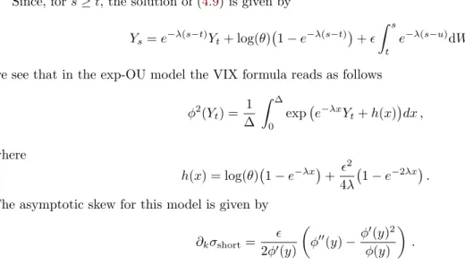
Since, fors≥t, the solution of (4.9) is given by
Ys=e−λ(s−t)Yt+ log(θ) 1−e−λ(s−t)
+ǫ
Z s
t
e−λ(s−u)dWu,
we see that in the exp-OU model the VIX formula reads as follows
φ2(Yt) = 1 ∆ Z ∆ 0 exp e−λxYt+h(x) dx , where h(x) = log(θ) 1−e−λx + ǫ 2 4λ 1−e −2λx .
The asymptotic skew for this model is given by
∂kσshort= ǫ 2φ′(y) φ′′(y)−φ′(y)2 φ(y) .
In Figure1we display the expansions ¯σN N,N = 2,3,4,together with the exact implied volatilities, relative to the following parameters: λ= 5.83, θ = 0.022, ǫ= 2.14, Y0 =−3.3. Notice that the implied volatility
curve is rather flat for both maturities. This is not unexpected, as in the exp-OU model the distribution of the VIX is approximately log-normal. For short (one week) time to maturity, the expansion order has no noticeable effect on the accuracy of the approximation, with an APE averaging to 0.04% and always below 0.3%. At one month to maturity, the fourth order expansion provides a neat improvement over the second and the third order expansions. Here, the average APE is 0.8% and never exceeds 0.9%.
MR-CEV SVV DMR DH exp-OU λ 1.6 λ1 2.26 λ1 5.5 λ1 0.179 λ 5.83 θ 0.125 λ2 1 λ2 0.1 λ2 1.303 θ 0.022 ǫ 3 θ1 0.0374 θ 0.078 θ1 0.007 ǫ 2.14 y 0.09 θ2 0.299 ǫ1 2.689 θ2 0.114 y −3.3 δ 1 ǫ2 1 ǫ2 0.502 ǫ1 1 ̺ 0.8 δ1 0.94 ǫ2 0.2 δ1 0.5 δ2 0.94 ̺ −0.8 δ2 0.5 ̺ 0.59 y1 0.03 y1 0.0324 y1 0.114 y2 0.03 y2 0.299 y2 0.110
Table 1: The table displays parameter specifications employed for the MR-CEV, SVV, DMR, DH and exp-OU models to generate the implied volatility curves plotted in Figure2.
MR-CEV model -0.22 -0.11 0 0.095 0.18 0.26 1 1.2 1.4 1.6 VIX T−t= 1 week -0.22 -0.11 0 0.095 0.18 0.26 1 1.2 1.4 VIX T−t= 1 month SVV model -0.22 -0.11 0 0.095 0.18 0.26 0.6 0.8 1 VIX T−t= 1 week -0.22 -0.11 0 0.095 0.18 0.26 0.6 0.8 1 VIX T−t= 1 month DMR model -0.22 -0.11 0 0.095 0.18 0.26 1 1.2 1.4 VIX T−t= 1 week -0.22 -0.11 0 0.095 0.18 0.26 0.8 1 1.2 VIX T−t= 1 month DH model -0.22 -0.11 0 0.095 0.18 0.26 0.6 0.8 1 1.2 1.4 VIX T−t= 1 week -0.22 -0.11 0 0.095 0.18 0.26 0.4 0.6 0.8 1 1.2 VIX T−t= 1 month exp-OU model -0.22 -0.11 0 0.095 0.18 0.26 0.7 0.8 0.9 1 VIX T−t= 1 week -0.22 -0.11 0 0.095 0.18 0.26 0.6 0.7 0.8 VIX T−t= 1 month
Figure 2: The figure plots the true implied volatilities generated by MR-CEV, SVV, DMR, DH and exp-OU models against the corresponding expansions of order 2 (red asterisks), 3 (blue triangles), and 4 (yellow circles). The curves are functions of log-moneyness log(K/FT
5
Conclusions
In this work we derive short-time asymptotic expansions for the VIX implied volatilities under the assumption that the VIX index evolves according to a purely diffusive, multidimensional Markov process. This modeling setup is general enough to include a large variety of the SV pricing models proposed in the financial literature. Pivotal for our approach is the technique by LPP, a perturbation methodology to approximate solutions to parabolic PDEs by expanding the infinitesimal generator of the underlying process. However, we need to develop non trivial generalizations suitable to cover the case of VIX options, as the dynamics of the underlying VIX futures are not explicitly known. Further complications arise from the fact that the relevant generators are fully degenerate, while previous asymptotic results by LPP postulate locally elliptic operators. We overcome these difficulties by proposing a double-layer version of this perturbation approach combined with a regularization technique known from the PDE literature. In particular, we establish rigorous error estimates and exact asymptotic results in the joint regime of short time-to-maturity and small moneyness. To illustrate the accuracy of our double-layer technique, we provide numerical implementations for a selection of model specifications.
A
Appendix
A.1
The approximating technique
In this appendix, we briefly describe the approximating technique by LPP, which is pivotal for the results derived in Section3. As already mentioned, this methodology has been developed through a series of papers gradually relaxing the underlying assumptions and broadening the domain of application. Following the pio-neering work ofHagan and Woodward(1999) and building upon PDEs perturbation theory and Dyson series (see, e.g.,Kevorkian and Cole(1981)),Pagliarani and Pascucci(2012) lay out the basic version of the tech-nique for univariate diffusions. Subsequently,Lorig et al.(2015) andLorig et al.(2017) derive expansions and small-time error bounds in a multivariate, uniformly parabolic setting while inPagliarani and Pascucci(2014) the results are generalized to locally parabolic operators. Recent generalizations byPagliarani and Pascucci
(2017) lead to asymptotic results valid in a joint regime of time-to-maturity and log-moneyness. In what follows, we summarize the construction of the approximations for prices and implied volatility, which can be performed under rather weak regularity assumptions. All the existing asymptotic accuracy results are left aside at this stage, as they do not directly apply to the VIX problem; some extensions will be presented in SectionA.2below to prove the results of Section3.
FixT0 >0, d∈ N0 and consider a continuous Rd+1-valued Markov processZ = (Zt1, . . . , Ztd+1)t∈[0,T0],
living on a filtered probability space (Ω,F,(Ft)0≤t≤T0,Q). The process Z represents a number of assets
and/or stochastic factors in a financial market where, for simplicity, interest rates and dividends are set to zero. The probability measure Q represents the risk-neutral measure adopted for any pricing purpose. Fix now a maturity date T ≤ T0, and consider a European style contract with maturity T and payoff
ϕ(z) =ϕ(zd+1), i.e., written solely on the (d+ 1)-th component of Z. Under the further assumption that
E[|ϕ(ZTd+1)|]<∞, the pricing function of the contract is given by
v(t, z;T) :=E[ϕ(ZTd+1)
The dependence of ϕ on a single factor is not a necessary condition for the methodology by LPP, which applies to more general payoffs. However, we work under this requirement as this is the only payoff type we consider in Section3. Throughout this section, we fixN∈N0and enforce the following standing assumption.
Assumption A.1. There exists a domainDZ ⊆Rd+1 such that
(i) The processZ is a local diffusion onDZ (see, e.g., Assumption 2.1 inPagliarani and Pascucci(2017)) with generatorAt locally given by
At=At(z) = 1 2 d+1 X i,j=1 aij(t, z)∂zizj + d+1 X i=1 ai(t, z)∂zi, (t, z)∈[0, T0[×DZ.
(ii) The coefficients aij, ai ∈ CN
P([0, T0[×DZ), where CPN denotes the usual parabolic space of order N,
i.e., the space of functions with derivatives up to the N-th order, where one derivative in tcompares to two derivatives in z(see, for instance, Chapter 10.1 inFriedman(1976)).
This assumption imposes rather mild demands. Many pricing models are defined via solutions, possibly stopped, of SDEs and such processes are indeed local diffusions, as shown byPagliarani and Pascucci(2017), Lemma 2.3. Also condition (ii) is fulfilled in nearly all practical applications, including the examples presented in this work. Note that no ellipticity condition is required at this stage.
A.1.1 Price approximations
Here we sketch the heuristic arguments leading to approximations of the pricing functionv(·,·;T) in (A.1). For a detailed description, we refer to Lorig et al.(2015), Section 3 . The starting point is the fact that typically–although not necessarily–v(·,·;T) satisfies
(∂t+At)v(·,·;T) = 0, on [0, T[×DZ, v(T, z;T) =ϕ(zd+1), z∈DZ. (A.2) To approximate the solution of (A.2) we undertake a formal perturbation approach: we fix (¯t,z¯)∈[0, T0[×DZ
and expand the operatorAtby replacing the functionsaij,ai with theirN-th orderparabolic Taylor series
around (¯t,¯z) as follows At≈A(¯t,t,0z¯)+ N X n=1 A(¯t,nt,z¯), (A.3) where At,n(¯t,z¯)=At,n(¯t,z¯)(z) = X 2q+|β|=n (t−¯t)q(z−z¯)β d+1 X i,j=1 ∂tqDzβaij(¯t,z¯) q!β! ∂zizj+ d+1 X i=1 ∂tqDβzai(¯t,z¯) q!β! ∂zi , 0≤n≤N. (A.4) Here, for any multi-indexβ ∈Nd0+1, we denote by
|β|=β1+· · ·+βd+1, β! =β1!· · ·βd+1!, Dzβ=∂zβ11· · ·∂
βd+1
zd+1 (A.5)
its length, its factorial, and the corresponding multi-derivative, respectively. Next, we consider an approxi-mate solution of the following type
v(t, z;T)≈ N X n=0 v(¯t,z¯) n (t, z;T), t∈[0, T], z∈DZ. (A.6)
Inserting (A.6) and (A.3) in (A.2), and collecting terms of the same order, we see that it is sensible to define (vn(¯t,z¯))0≤n≤N via a sequence of nested Cauchy problems. More precisely,v(¯0t,z¯) is defined as the solution of
(∂t+A(¯t,t,0z¯))v0(¯t,z¯)= 0, on [0, T[×Rd+1, v(¯0t,z¯)(T, z;T) =ϕ(zd+1), z∈Rd+1. (A.7)
while, for 1≤n≤N, the functionv(¯nt,z¯)is recursively defined as the solution of (∂t+A(¯t,t,0z¯))vn(¯t,z¯)=−Pn h=1A (¯t,z¯) t,h v (¯t,z¯) n−h, on [0, T[×Rd+1, v(¯nt,z¯)(T, z;T) = 0, z∈Rd+1.
Since, by definition, the zero order operatorA(¯t,t,0z¯)has constant coefficients, the zero order termv(¯0t,z¯)is given
by v0(¯t,¯z)(t, z;T) =v (¯t,z¯) 0 (t, zd+1;T) := Z Rd Γ0(t, zd+1;T, ξ)ϕ(ξ)dξ, (A.8)
where Γ0(t, zd+1;T, ξ) is the univariate Gaussian density
Γ0(t, zd+1;T, ξ) := p 1 2π(T−t)exp − ξ−zd+1−ad+1(¯t,z¯)(T−t) 2 2ad+1d+1(¯t,z¯)(T −t) ! .
Following Theorem 2.6 inLorig et al.(2017), the remaining correcting terms (v(¯nt,z¯))1≤n≤N are given by
v(¯nt,z¯)(t, z;T) :=L(¯nt,z¯)(t, T, z)v
(¯t,z¯)
0 (t, z;T), (A.9)
whereL(¯nt,¯z)(t, T, z) denotes the differential operator acting on thez-variable and defined as
L(¯nt,¯z)(t, T, z) := n X h=1 Z T t ds1 Z T s1 ds2· · · Z T sh−1 dsh X i∈In,h G(¯it,z¯) 1 (t, s1, z)· · ·G (¯t,¯z) ih (t, sh, z), with1 In,h:={i= (i1, . . . , ih)∈Nh|i1+· · ·+ih=n}, 1≤h≤n,
and the operatorG(¯nt,z¯)(t, s, z) is defined as
G(¯nt,¯z)(t, s, z) :=A(¯s,nt,¯z) z+m(¯t,z¯)(t, s) +C(¯t,z¯)(t, s)∇z,
withm(¯t,z¯)(t, s) andC(¯t,z¯)(t, s) being, respectively, the vector and the matrix whose components are given by
m(¯it,z¯)(t, s) := (s−t)ai t,¯¯z
, C(¯ijt,¯z)(t, s) := (s−t)aij ¯t,z¯
, i, j= 1, . . . , d.
These reasonings lead to the following definition.
Definition A.2. Let AssumptionA.1be in force, and consider the pricing functionv(t, z;T) given in (A.1). For a fixed (¯t,z¯)∈[0, T0[×DZ, we define theN-th order approximation centered at(¯t,z¯)ofvas the following
function ¯ v(¯Nt,z¯)(t, z;T) = N X n=0 vn(¯t,¯z)(t, z;T), (A.10)
wherev0(¯t,¯z)is given by (A.7) and (v (¯t,z¯)
n )1≤n≤N are given by (A.9). 1
A few remarks are in place
Remark A.3. (i) Approximations similar to the one presented here can be based on any polynomial ex-pansion of the coefficientsaij,ai. See e.g. Lorig et al.(2015) for a discussion on alternative expansions. We focus only on the parabolic Taylor expansion (A.4) as this is the most suitable for the purpose of this work, as clarified in Remarks 3.7and3.9.
(ii) From expression (A.8) we see that the leading termv0(¯t,¯z)admits a closed form expression if the integral of the final datum ϕ(zd+1) against a Gaussian density is explicitly computable. In such a case, also
the integral representations (A.9) of the higher order terms (vn(¯t,z¯))1≤n≤N are explicitly computable.
In other words, the approximation is explicitly computable whenever the payoff function allows for a closed form formula in the Black-Scholes world.
(iii) Notice that definition A.2 only requires the existence of an operator At with coefficients which are differentiable enough. In particular, no ellipticity assumption is needed and the N-th order approxi-mation ¯vN(¯t,z¯)can be constructed irrespective on whether the true pricing functionvsatisfies the Cauchy problem (A.2).
A.1.2 Implied volatilities approximations
In this section we briefly recall how the approximation (A.10), when applied to a call option payoff, leads to a closed form implied volatility approximation. Here, we assume that the d+ 1 component Zd+1 of
the underlying process Z represents the log-value of the futures price of an asset with settlement date T
coinciding with the maturity the call. So the process (eZd+1
t )0
≤t≤T is a martingale, which in turn entails the
following condition on the generator ofZ:
ad+1(t, z) =−
1
2ad+1d+1(t, z), (t, z)∈[0, T[×DZ.
Consistent with the notation of Section3, we denote byu(t, z;T, k) the pricing function of a call with expiry
T and log-strikek, i.e.,
u(t, z;T, k) =E[(eZTd+1−ek)+|Zt=z],
and by σ(t, z;T, k) its implied volatility. Furthermore, we denote by (u(¯nt,z¯))0≤n≤N the terms of the N-th
order approximation ofu, centered at (¯t,z¯), and we denote byuBS(σ;T−t, zd
+1, k) the call price under the
B&S model as defined in (3.4). We are now ready to formulate the following concept.
Definition A.4 (The LPP conversion). Let Assumption A.1 be in force and fix (¯t,z¯)∈[0, T]×DZ. We define theN-th order approximation centered at(¯t,z¯)of the implied volatility σ(t, z;T, k) as the function
¯ σ(¯Nt,z¯)(t, z;T, k) = N X n=0 σ(¯nt,z¯)(t, z;T, k), where σ0(¯t,¯z)(t, z;T, k)≡ p ad+1d+1(¯t,z¯),
while the remaining terms (σn(¯t,¯z))1≤n≤N are defined recursively as follows:
σn(¯t,¯z)= u(¯nt,¯z) ∂σuBS σ(¯t,z¯) 0 − 1 n! n X h=2 Bn,h 1!σ1(¯t,z¯),2!σ (¯t,z¯) 2 , . . . ,(n−h+ 1)!σ (¯t,z¯) n−h+1 ∂σhuBS σ(¯0t,z¯) ∂σuBS σ(¯t,¯z) 0 , (A.11)