rule-focusing methodology
Julien Blanchard, Fabrice Guillet, Henri Briand
To cite this version:
Julien Blanchard, Fabrice Guillet, Henri Briand. Interactive visual exploration of association
rules with rule-focusing methodology. Knowledge and Information Systems (KAIS), Springer,
2007, 13 (1), pp.43-75.
<
10.1007/s10115-006-0046-2
>
.
<
hal-00420938
>
HAL Id: hal-00420938
https://hal.archives-ouvertes.fr/hal-00420938
Submitted on 30 Sep 2009
HAL
is a multi-disciplinary open access
archive for the deposit and dissemination of
sci-entific research documents, whether they are
pub-lished or not.
The documents may come from
teaching and research institutions in France or
abroad, or from public or private research centers.
L’archive ouverte pluridisciplinaire
HAL
, est
destin´
ee au d´
epˆ
ot et `
a la diffusion de documents
scientifiques de niveau recherche, publi´
es ou non,
´
emanant des ´
etablissements d’enseignement et de
recherche fran¸
cais ou ´
etrangers, des laboratoires
Interactive Visual Exploration of
Association Rules with Rule Focusing
Methodology
Julien Blanchard, Fabrice Guillet and Henri Briand
KnOwledge & Decision Team (KOD)
LINA – FRE CNRS 2729, Polytechnic School of Nantes University, France
Abstract. On account of the enormous amounts of rules that can be produced by data mining algorithms, knowledge post-processing is a difficult stage in an association rule discovery process. In order to find relevant knowledge for decision-making, the user (a decision-maker specialized in the data studied) needs to rummage through the rules. To assist him/her in this task, we here propose therule focusing methodology, an interac-tive methodology for the visual post-processing of association rules. It allows the user to explore large sets of rules freely by focusing his/her attention on limited subsets. This new approach relies on rule interestingness measures, on a visual representation, and on interactive navigation among the rules. We have implemented the rule focu-sing methodology in a prototype system called ARVis. It exploits the user’s focus to guide the generation of the rules by means of a specific constraint-based rule-mining algorithm.
Keywords: knowledge discovery in databases, association rules, post-processing, in-teractive visualization, rule focusing, constraint-based mining, interestingness mea-sures, neighborhood of rules
1. Introduction
Among the knowledge models used in Knowledge Discovery in Databases (KDD), association rules (Agrawal et al, 1993) have become a major concept and have re-ceived significant research attention. Association rules are implicative tendencies
X →Y whereX andY are conjunctions of items (boolean variables of the form
databaseAttribute=value). The left-hand sideXis the antecedent of the rule and
Received Oct 7, 2004 Revised Nov 7, 2005 Accepted May 3, 2006
the right-hand side Y the consequent. Such a rule means that most of the re-cords which verify the antecedent in the database verify the consequent too. For instance, in market basket analysis where the data studied are the customers’ transactions in a supermarket, an association rule {pizza, crisps} → {beer}
means that if a customer buys a pizza and crisps then (s)he most probably buys beer too. Since the pioneering algorithm of Agrawal, called Apriori (Agrawal and Srikant, 1994), many algorithms have been proposed for association rule mining (cf. Hipp et al (2000) for a survey). They generally produce very large amounts of rules. This is due to the unsupervised nature of association rule discovery. Indeed, because the user does not know precisely enough what (s)he is looking for to express it with the data terminology, (s)he does not make his/her goals ex-plicit and does not specify any endogenous variable. Thus, the algorithms search all the valid associations existing in the database and generate an amount of rules exponentially growing with the number of items.
A crucial step in association rule discovery is post-processing, i.e., the in-terpretation, evaluation and validation of the rules in order to find interesting knowledge for decision-making. Because of the oversized amounts of rules, the post-processing stage often turns out to be a second mining challenge called ”knowledge mining”. While data mining is automatically computed by combi-natorial algorithms, the knowledge mining stage is manually done by the user (a decision-maker specialized in the data studied). In practice, it is very difficult for users to rummage through the rules and find interesting ones in a corpus that can hold hundreds of thousands of rules, or even millions of rules with large business databases.
Many authors have stressed that the KDD process is by nature highly ite-rative and interactive and requires user involvement (Silberschatz and Tuzhi-lin, 1996) (Fayyad et al, 1996). In particular, Brachman and Anand (1996) have pointed out that in order to efficiently assist the users in their search for inter-esting knowledge, the KDD process should be considered not from the point of view of the discovery algorithms but from that of the users’, as a human-centered decision support system. The human-centered approaches aim at creating a re-troaction loop between the user and the system which constantly takes into account the information processing capacities of the user (cf. Bisdorff (2003) for examples of applications). Adopting Brachman & Anand’s point of view, in this article we propose the rule focusing methodology, a human-centered methodo-logy for the post-processing of association rules. The rule focusing methodomethodo-logy allows the user to explore large sets of rules by focusing his/her attention on suc-cessive limited subsets. The methodology relies on severalneighborhood relations
that connect the rules among them according to the user’s semantics. With these relations, the user can navigate freely among the subsets of rules and thus drive the post-processing. In this way, a voluminous set of rules is explored subset by subset so that the user does not need to appropriate it entirely. Our approach combines:
– rule interestingness measures to filter and sort the rules,
– a visual representation to make comprehension easier,
– interactivity based on the neighborhood relations to guide the post-processing. The rule focusing methodology can be used in two ways. First, it can be ap-plied after association rule mining, as a pure post-processing technique. This is also called post-analysis or a posteriori filtering of rules (Hipp and Gntzer, 2002).
Secondly, it can be applied during association rule mining, as an interactive mi-ning technique conducted by the user. Effectively, the rule focusing methodo-logy induces a constraint-based mining algorithm. A constraint-based rule-mining algorithm exploits constraints that the user gives to specify which kind of rules (s)he wants to find (cf. for example Srikant et al (1997), Ng et al (1998), Goethals and Van den Bussche (2000), Jeudy and Boulicaut (2002), Ordonez et al (2006)). Syntactic constraints (constraints specifying the items that must occur or not in the rule) and interestingness measure threshold constraints are the most commonly used constraints, but more general studies concern the so-called anti-monotone and succinct constraints (Ng et al, 1998), and the monotone constraints (Grahne et al, 2000) (Bonchi et al, 2005). Constraints allow to si-gnificantly reduce the exponentially growing search space of association rules1.
Thus, the constraint-based algorithms can mine dense data more efficiently than the classical Apriori-like algorithms (the FP-growth-based algorithms of (Han et al, 2000) can mine dense data too, but they use a condensed representation of the data and require that it holds in memory). Besides, with appropriate constraints, the constraint-based algorithms can discover very specific rules which cannot be mined by the Apriori-like algorithms (the constraint-based algorithms can use low support thresholds for which Apriori-like algorithms are intractable). These rules are often very valuable for the users because they were not even thought of beforehand (Freitas, 1998). For these reasons, we use a constraint-based rule-mining algorithm to implement the rule focusing methodology in the prototype system described in this article. This specific algorithm extracts the rules inter-actively according to the user’s focus. Note that using the rule focusing metho-dology as a pure post-processing technique or as an interactive mining technique is only a choice of implementation. The methodology does not depend on it.
The remainder of this article is organized as follows. In the next section we present a survey on association rule evaluation, exploration, and visualiza-tion. Then we describe the Information Visualization field of research, and in particular we compare 2D and 3D visualizations. Section 4 is dedicated to the study of cognitive constraints of the user during rule post-processing. From these constraints, in section 5, we define the rule focusing methodology. Section 6 des-cribes the prototype system implementing our methodology: ARVis, a visual tool for association rule mining and post-processing . In section 7, we give an example of rule post-processing with ARVis. It comes from a study made with the firm PerformanSe SA on human resource management data. Finally we give our conclusion in section 8.
2. Survey on association rule evaluation, exploration, and
visualization
At the output of the data mining algorithms, the sets of association rules are simple text lists. Each rule consists of a set of items for the antecedent, a set of items for the consequent (sets of items are called itemsets), and the numerical values of two interestingness measures, support and confidence (Agrawal et al, 1993). Support is the proportion of records which verify a rule in the database;
1 Choosing the best way of harnessing multiple constraints whatever the data is still an open problem.
it evaluates the generality of the rule. Confidence (or conditional probability) is the proportion of records which verify the consequent among those which verify the antecedent; it evaluates the validity of the rule (success rate).
Three kinds of approaches aim at helping the user appropriate large sets of association rules:
– the user can filter and order the rules with other interestingness measures;
– the user can browse the large sets of rules with interactive tools or query languages;
– the user can visualize the rules.
2.1. Rule interestingness measures
It is now well-known that the support-confidence framework is rather poor to evaluate the rule quality (Silverstein et al, 1998) (Bayardo and Agrawal, 1999) (Tan et al, 2004). Numerous rule interestingness measures have been proposed to complement this framework. They are often classified into two categories: the subjective (user-oriented) ones and the objective (data-oriented) ones. Subjective measures take into account the user’s a priori knowledge of the data domain (Liu et al, 2000) (Silberschatz and Tuzhilin, 1996) (Padmanabhan and Tuzhilin, 1999). On the other hand, the objective measures do not depend on the user but only on objective criteria such as data cardinalities or rule complexity. Depending on whether they are symmetric (invariable by permutation of antecedent and consequent) or not, they evaluate correlations or rules.
There exist two significant configurations in which the rules appear non-directed relations and therefore can be considered as neutral or non-existing (Blanchard, 2005):
– theindependence, i.e., when the antecedent and consequent are independent;
– what we call the equilibrium, i.e., when examples and counter-examples are equal in numbers (maximum uncertainty of the consequent given that the antecedent is true).
Thus we distinguish two different but complementary aspects of the rule interestingness: the deviation from independence and the deviation from equili-brium. The objective measures of interestingness can be classified into two classes (Blanchard et al, 2005) (Blanchard et al, 2005):
– the measures of deviation from independence, which have a fixed value at independence, such as rule-interest (Piatetsky-Shapiro, 1991), lift (Silverstein et al, 1998), conviction (Brin et al, 1997), Loevinger index (Loevinger, 1947), implication intensity (Gras, 1996) (Blanchard et al, 2003);
– the measures of deviation from equilibrium, which have a fixed value at equili-brium, such as confidence (Agrawal et al, 1993), Sebag and Schoenauer index (Sebag and Schoenauer, 1998), IPEE (Blanchard et al, 2005).
These two kinds of measures are complementary (in particular, they do not create the same preorder on rules) (Blanchard, 2005) (Blanchard et al, 2005). A rule can have a good deviation from independence with a bad deviation from equilibrium, and conversely. Regarding the deviation from independence, a rule
A →B with a good deviation means ”When A is true, then B ismore often true” (more than usual, i.e. more than without any information about A). On
the other hand, regarding the deviation from equilibrium, a ruleA→B with a good deviation means ”WhenA is true, thenB isvery often true”. Deviation from independence is a comparison relatively to an expected situation, whereas deviation from equilibrium is an absolute statement. The measures of deviation from independence are useful to discover associations between antecedent and consequent (do the truth ofAinfluence the truth ofB?), while the measures of deviation from equilibrium are useful to take decisions or make predictions about
B (knowing or supposing thatAis true, isB true or false?) (Blanchard, 2005).
2.2. Interactive browsing of rules
Interactive tools of the type ”rule browser” have been developed to assist the user in the post-processing of association rules. First, Klemettinen et al (2004) present a browser with which the user reaches interesting rules by adjusting thresholds on interestingness measures and applying syntactic constraints (tem-plates). Secondly, Liu et al (1999) propose a rule browser which is based on subjective interestingness measures and exploits the user’s a priori knowledge of the data domain to present the rules. The user expresses his/her knowledge under the form of relations and then the tool classifies the rules in different ca-tegories according to whether they confirm or not the user’s beliefs. Finally, in (Ma et al, 2000), the user explores a summary of the rules. (S)he can access the rules by selecting elements in the summary. The main limit of all these tools lies in the textual representation of the rules which does not suit the study of large amounts of rules described by numerous interestingness measures.
More recently, a rule browser equipped with numerous functionalities has been presented in (Fule and Roddick, 2004). It allows to filter the rules with syn-tactic constraints that are more or less general since they can take into account an item taxonomy. The tool also enables the user to program any interestingness measure to order and filter the rules. Besides, the user can save the rules that (s)he judges interesting during the exploration. Another rule browser is presented in (Tuzhilin and Adomavicius, 2002), but it is not a generic tool. It is dedicated to the analysis of gene expression data coming from DNA microarrays, and relies on a very complete system of syntactic constraints which can take into account a gene taxonomy.
Within the framework of inductive databases (Imielinski and Mannila, 1996), several rule query languages have been proposed, such as DMQL (Han et al, 1996), MINE RULE (Meo et al, 1998), MSQL (Imielinski and Virmani, 1999), or XMINE (Braga et al, 2002). They allow to mine (by means of constraint-based algorithms) and post-process rules interactively under the user’s guidance. However, as regards rule post-processing, the query languages are not very user-friendly (cf. (Botta et al, 2002) for an experimental study).
2.3. Visualizing the rules
Visualization can be very beneficial to KDD (Fayyad et al, 2001). Visualization techniques are indeed an effective means of introducing human subjectivity into each stage of the KDD process while taking advantage of the human percep-tual capabilities. The information visualization techniques can either be used as knowledge discovery methods on their own, which is sometimes called ”visual
Fig. 1.An item-to-item matrix showing the rules{crisps} → {pizza}and{pizza} → {beer}
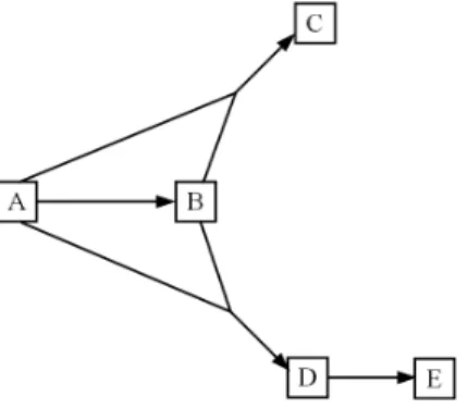
Fig. 2.A rule graph with items as nodes, showing the rulesA→B,AB→C,AB→D, and
D→E
data mining” (Keim, 2002), or they can collaborate with data mining algorithms to facilitate and speed up the analysis of data, intermediate results, or discovered knowledge (Aggarwal, 2002) (Schneiderman, 2002) (Han et al, 2003). Associa-tion rule visualizaAssocia-tion comes within this latter case. It must be noticed that the methods and tools presented below are generally supplied with basic functiona-lities for ordering and filtering the rules on items and on a few interestingness measures.
A first rule visualization method consists in using a matrix representation. Hofmann and Wilhelm (2001) and the Quest research group (Agrawal et al, 1996), as well as the software programs DBMiner (Han et al, 1997), SGI MineSet (Brunk et al, 1997), DB2 Intelligent Miner Visualization (?), and Enterprise Miner (?), give different implementations of it. In an item-to-item matrix (figure 1), each line corresponds to an antecedent item and each column to a consequent item. A rule between two items is symbolized in the matching cell by a 2D or 3D object whose graphical characteristics (generally size and color) represent the interestingness measures. This visualization technique has been improved into rule-to-item matrices (Wong et al, 1999) whose cluttering is lower and which allow a more efficient representation of rules with more than two items. The main limit of these approaches is that the matrices reach considerable sizes in case of large sets of rules over numerous items.
Sets of association rules can be also visualized by using a directed graph (Klemettinen et al, 2004) (Han et al, 1997) (Rainsford and Roddick, 2000) (?), the nodes and edges respectively representing the items and the rules (cf. figure
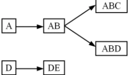
Fig. 3.A rule graph with itemsets as nodes, showing the rulesA→B,AB→C,AB→D, andD→E
The represented rules involve the items heineken, coke, and chicken in antecedent, and
sardinesin consequent. Antecedent and consequent are respectively read on the horizontal and vertical axes. The first rectangle on the left shows that the rule{heineken= 0, coke= 0, chicken= 0} → {sardines= 1}has a confidence of about 40% (red part of the rectangle), while the opposite rule{heineken= 0, coke= 0, chicken= 0} → {sardines= 0}has a confi-dence of 60% (grey part of the rectangle). The support of the rules is proportional to the area (red or grey) of the rectangles. The rectangle on the right indicates that the confidence of the rule{heineken= 1, coke= 1, chicken= 1} → {sardines= 1}is about 100%.
Fig. 4.Mosaic display for association rules (from Hofmann et al (2000))
2 where letters denote items). The interestingness measures are symbolized on the edges, for instance with color or thickness. The graph representation is very intuitive but it has two main drawbacks. First, it makes transitivity appear among the rules whereas, in the general case, the rules are not transitive (with most measures, rule interestingness does not spread transitively). Secondly, it does not suit the visualization of large sets of rules over numerous items either. Indeed, the graph is then overloaded with nodes and crossing edges, all the more when rules with more than two items are considered. To improve the rule visualization, the same representation method has been used in 3D with a self-organization algorithm to guarantee a more efficient graph layout (Hao et al, 2001). Also we have proposed in (Kuntz et al, 2000) a dynamic rule graph which is a subgraph of the itemset lattice. In this graph, the nodes do not represent the items but the itemsets so that a ruleAB→C is symbolized by an edge between the nodes AB and ABC (figure 3). The resulting graph is acyclic with more nodes but fewer edge crossings. The user can dynamically develop the graph as (s)he wishes by clicking on the nodes.
All the visual representations described so far are based on rule syntax (i.e. the items). A different approach is proposed in (Unwin et al, 2001), where the
representation is based on interestingness measures. This representation is a scatterplot between support and confidence where each point is colored according to density estimation. The user can query any point to display the names of the rules represented by the point (rules with close supports and confidence). The main advantage of such a representation is that it can contain a great number of rules. However, several rules can be represented by one and only one point, which does not facilitate the task of the users when they search for rules using items as criteria. This approach is the closest to the one we propose in this paper, which also uses a spatial mapping to highlight the interestingness measures.
Other methods have been proposed to represent association rules. Neverthe-less, they do not deal with the visualization of the whole rule set but with the visualization of a pattern of rules (a group of rules with given items in antecedent and consequent). These methods allow a thorough study of a restricted number of rules, making their interpretation easier and helping to understand their oc-currence context. We can quote for example Hofmann et al.’s mosaic plots (2000) for rules with categorical attributes (figure 4), or Fukuda et al (2001) and Han et al (2003) for numerical rules. Also some techniques inspired from parallel co-ordinates have been considered to visualize patterns of classification rules (Han et al, 2000) or association rules (Kopanakis and Theodoulidis, 2001).
3. Information visualization
3.1. Context
Information visualization(Card et al., 1999) (Spence, 2000) consists in represen-ting abstract data under a visual form in order to improve cognition for a given task, that is to say the acquisition and use of new knowledge. The core of infor-mation visualization is visual encoding, i.e., the mapping of data tables to visual structures in a 2D or 3D space (Card et al., 1999). The visual structures have several graphical properties such as position, length, area, hue, brightness, satu-ration, shape, texture, angle, curvature... They can be zero-dimensional (points), one-dimensional (lines), two-dimensional (surfaces), or three-dimensional (vo-lumes).
Several authors proposed classifications of visual encodings in order to show which ones are appropriate according to the data variables to be represented. Among these works, those of Cleveland and McGill (1984), Tufte (1983), and then Wilkinson (1999) are references for statistical graphs (charts). A second trend stems from cartography, with the works of McEachren (1995) and Bertin whoseSemiology of Graphics (Bertin, 1967-1983) is considered as the first and most influential structural theory of graphics (Wilkinson, 1999). As regards the visual representation of quantitative variables, the two trends agree that the best encodings are done with position (Bertin, 1967-1983) (Cleveland and McGill, 1984) (McEachren, 1995) (Card et al., 1999) (Wilkinson, 1999). However, the two trends mainly differ about the use of surfaces to represent quantitative variables: this use is not advisable with statistical graphs whereas it is standard practice in cartography. In particular, Cleveland and McGill (1984) propose a hierarchy of visual encodings saying that surface is little appropriate (less than length) to represent quantities. This point of view is based on Stevens’s law in psychophysics according to which the perceived quantities are not linearly related to the actual quantities with surface (Baird, 1970). On the other hand, Bertin points out that
before the variation of length, the variation of surface is the sensitive stimulus of the variation of size (Bertin, 1967-1983).
The visualization we propose in this article is not a map, and even less a statistical graph: this is a 3D virtual world. With the increase in the capacities of personal computers, the 3D virtual worlds have become common in informa-tion visualizainforma-tion (Chen, 2004). Associated with navigainforma-tion operators (viewpoint controls), they have shown to be efficient for browsing wide information corpuses such as large file system hierarchies with Silicon Graphics’ FSN (re-used in Mine-Set for the visualization of decision trees), hypertext document graphs with Har-mony (Andrews, 1995), or OLAP cubes with DIVE-ON (Ammoura et al, 2001)] (cf. Chen (2004) for other examples of applications). While a 2D representation is restricted to the two dimensions of the screen, the additional dimension in a 3D virtual world offers a viewpoint towards infinity, creating a wide works-pace capable of containing a large amount of information (Card et al., 1999). In this workspace, the most important information can be placed in the foreground (most visible objects) and thus be highlighted compared to the less important information placed behind it (less visible objects). This is the reason why the 3D representations are sometimes considered as focus+context approaches. Moreo-ver, 3D enables to exploit volumes as objects in the visualization space. It allows to benefit from more graphical properties for the objects and thus to represent even more information.
3.2. 2D or 3D?
The choice between 2D and 3D representations for information visualization is still an open problem (Card et al., 1999) (Chen, 2004). This is especially due to the fact that the efficiency of a visualization is highly task-dependent (Carswell et al, 1991). Besides, while 3D representations are often more attractive, 2D has the advantage of a long and fruitful experience in information visualization. In fact, few research works are dedicated to the comparison between 2D and 3D. As regards the static (non interactive) visualization of statistical graphs, the 3D re-presentations have generally not been advisable since the influential publications of Tufte (1983) and Cleveland and McGill (1984). Nevertheless, the psychophy-sics experiments of Spence (1990) and Carswell et al (1991) show that there is no significant difference of accuracy between 2D and 3D for the comparison of numerical values. In particular, Spence points out that this is not the apparent dimensionality of visual structures which counts (2 for a surface, 3 for a volume) but the actual number of parameters that show variability (Spence, 1990). In his experiments, whatever the apparent dimensionality of visual structures, Ste-vens’s law is almost always the same when only one parameter actually varies (Stevens’s law exponents are very close to 1). Under some circumstances, infor-mation may even be processed faster when represented in 3D rather than in 2D. As regards the perception of global trends in data (increase or decrease), the experimental results of Carswell et al (1991) also show an improvement in the answer times with 3D but to the detriment of accuracy.
Other works compare 2D and 3D within the framework of interactive vi-sualization. Cockburn and McKenzie (2001) study the storage and retrieval of bookmarked web-pages in a 2D or 3D visualization space. With the 2D interface, the processing times of the users are shorter but not significantly. On the other hand, the subjective assessment of the interfaces shows a significant preference
for 3D (which Spence (1990) and Carswell et al (1991) also sense but without assessing it). Finally, Ware and Franck (1996) compare the visualization of 2D graphs and 3D graphs. Their works show a significant improvement in intelligi-bility with 3D. More precisely, their experiment consists in asking users whether there is a path of length two between two nodes randomly chosen in a graph. With the 3D graphs, the error rate is reduced by 2.2 for comparable answer times. With stereoscopic display, the error rate is even reduced by 3. One gene-rally considers that only stereoscopy allows fully exploiting the characteristics of the 3D representations.
4. Cognitive constraints of the user during rule
post-processing
4.1. User’s task
During the post-processing of the rules, the user is faced with long lists of rules described by interestingness measures. The user’s task is then to rum-mage through the rules in order to find interesting ones for decision-making. To do so, (s)he needs to interpret the rules in the business semantics and to evaluate their quality. The two decision indicators are therefore the rule syn-tax and the interestingness measures. The user’s task is difficult for two reasons. First, the profusion of rules at the output of the data mining algorithms prevents any exhaustive exploration. Secondly, on account of the unsupervised nature of association rule discovery, it is generally not feasible for the user to obviously formulate constraints which would isolate relevant rules directly.
4.2. Cognitive hypotheses of information processing
On account of the human ”bounded rationality” hypothesis (Simon, 1979), a decision process can be seen as a search for a dominance structure. More precisely, the decision-maker faced with a set of multiattribute alternatives tries to find an alternative (s)he considers dominant over the others, i.e., an alternative (s)he thinks better than the others according to his/her current representation of the decision situation (Montgomery, 1983). This type of models of decision process can be transferred to the post-processing of association rules by considering the rules as a particular kind of alternatives with items and interestingness measures as attributes. According to Montgomery, the decision-maker isolates a limited subset of potentially useful alternatives and makes comparisons among them. This can be done iteratively during the decision process. More precisely, he has pointed out that: ”The decision process acquires a certain directionality in the sense that certain alternatives and attributes will receive more attention than others [...] The directionality of the process may be determined more or less consciously. Shifts in the directionality may occur several times in the process, particularly when the decision-maker fails to find a dominance structure”.
Furthermore, a KDD methodology called ”attribute focusing” has been pro-posed in (Bhandari, 1994). It results from experimental data concerning the user’s behavior in the discovery process. This methodology is based on a filter which automatically detects a small number of potentially interesting attributes.
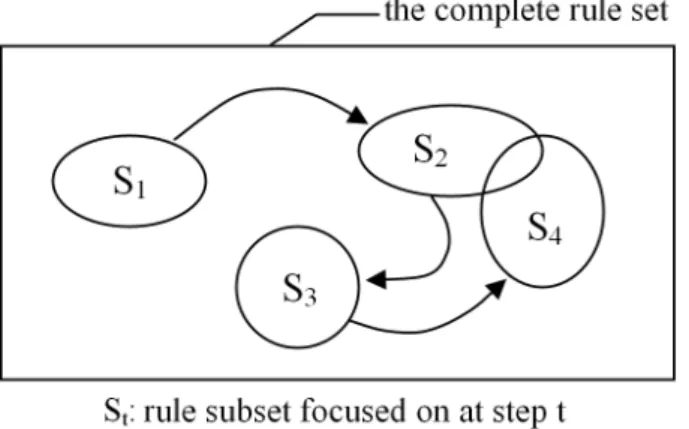
Fig. 5.Navigation among successive subsets of rules with the rule focusing methodology
The filter guides the user’s attention on a small, and therefore more intelli-gible, subset of the database. The importance of focusing on a small number of attributes in human information processing has also been widely confirmed with works on decision strategies (cf. for example the moving basis heuristics in (Barthelemy and Mullet, 1992)). Indeed, on account of his/her limited cognitive abilities, the decision-maker examines only a small amount of information at each moment.
From these different works on human information processing, we establish three principles on which our rule focusing methodology relies:
P1. enabling the user to focus his/her attention on a limited subset of rules with a small number of attributes (items and interestingness measures),
P2. enabling the user to make comparisons among the rules in the subset,
P3. enabling the user to shift the subset of rules (s)he is focusing on at any time during the post-processing, until (s)he is able to validate some rules and reach a decision.
5. Rule focusing methodology
The idea of developing therule focusingmethodology has arisen from our earlier works on the visualization of rule sets by graphs (Kuntz et al, 2000). The me-thodology consists in letting the user navigate freely inside the large set of rules by focusing on successive limited subsets via a visual representation of the rules and their measures. In other words, the user gradually drives a series of visual local explorations according to his/her interest for the rules (figure 5). Thus, the rule set is explored subset by subset so that the user does not need to appro-priate it entirely. At each navigation2 step, the user must make a decision to
choose which subset to visit next. This is the way subjectivity is introduced into the post-processing of the rules. The user acts here as an exploration heuristics.
2 We call ”navigation” the fact of going from one subset to another, while ”exploration” refers to the whole process supervised by our methodology, i.e., the navigation among the subsets and the visits (local explorations) of the subsets.
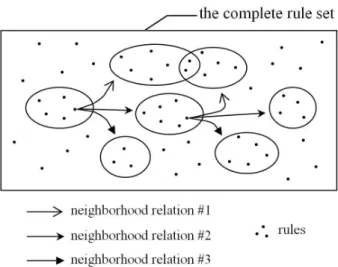
Fig. 6.A neighborhood relation associates each rule to a subset of rules
Exploiting a human heuristics is coherent since the function to be optimized, i.e. the user’s interest, is subjective.
The rule focusing methodology integrates the cognitive principles of section 4.2 in the following way:
– Relations allow to focus on the subsets and to navigate among them (principles P1 and P3). We call themneighborhood relations.
– The user visualizes the subsets to visit them, and in particular to compare the rules (principle P2).
Both the neighborhood relations and the visualization technique must take into account the two decision indicators involved in the user’s task: the rule syntax and the interestingness measures (cf. section 4.1).
5.1. Neighborhood relations among rules
The neighborhood relations determine the way the subsets of rules are focused on (cognitive principle P1) and the way the user can go from one subset to another (cognitive principle P3). They are a fundamental element of the rule focusing methodology since they are the vectors of the navigation for the user. These relations are defined in the following way: a neighborhood relation associates each rule from the complete set of rules to a limited subset of rules called neighbors (figure 6). So withxrelations, the user can reachxneighboring subsets of rules from one rule, and from a subset containingy rules (s)he can reachx.y possible neighboring subsets. To navigate from one subset to another, the user must make two choices: which neighborhood relation to apply, and on which rule.
In mathematical terms, the neighborhood relations are binary relations over the complete set R of the rules extracted by the data mining algorithms. Still with the aim of being appropriate to the user’s task, we choose neighborhood relations which have a pertinent meaning for the user:
∀(r1, r2)∈R2,
neighborOf(r1, r2)⇔ (the user judges thatr1 is close tor2from a point of view)
This introduces user semantics into the navigation among the rules. Any rela-tion could be considered provided it makes sense for the user. Consequently, the relations have to be defined with his/her help before starting the rule post-processing.
Here are for example four possible neighborhood relationsneighborOf(r1, r2):
1. r1is neighbor ofr2if and only ifr1 andr2have the same conclusion;
2. r1is neighbor ofr2if and only ifr1 is an exception ofr2;
3. r1 is neighbor of r2 if and only if the antecedent of r1 is more general than
that ofr2;
4. r1 is neighbor of r2 if and only if r1 has the same support and confidence as r2to within about 0.05.
The neighborhood relations 1, 2, and 3 are based on the rule syntax, while relation 4 is based on two interestingness measures. Furthermore, relation 1 is an equivalence relation, whereas relation 2 is neither reflexive, nor symmetric, nor transitive. Relation 3 is only transitive, and relation 4 is reflexive and symmetric but not transitive.
Let us assume that the user applies a neighborhood relation Π. From a rule
r, (s)he can reach the subsetS of all the rules that are neighbors ofraccording to Π. We call r the ”transitional rule” because it allows to navigate from one subset to another. Depending on the reflexivity of the relation Π chosen,S can or cannot contain the transitional ruler.
The originality of our methodology in comparison with the existing rule ex-ploration techniques (described section 2.2) mainly lies in the concept of neigh-borhood relation. With a query language or an interactive interface like a rule browser, the user can reach any subset of rules but (s)he must explicitly spe-cify the constraints which delimit it. With the rule focusing methodology, the constraint specification is implicit since it is hidden in the neighborhood re-lations. Actually, the neighborhood relations can be seen as generalizations of constraints (classes of constraints). We think that the user’s task is made easier with neighborhood relations than with explicit constraints. For example, let us imagine the following exploration scenario:
The user finds an interesting ruleABC→D (where letters denote items). (S)he thinks that the combination of these four items is very pertinent but (s)he would like to change the order of the items and verify whether the rules ABD → C,
ACD→B, andBCD→A(and why not the rules AB→CD,AC→BD and so on as well) are better evaluated by the interestingness measures.
With the rule focusing methodology, the user can carry out this scenario in just one interaction. (S)he only needs the neighborhood relation ”r1 is neighbor
ofr2 if and only ifr1 andr2 have the same items”. On the other hand, with a
query language or a rule browser, the user has to write a series of appropriate queries or to specify a series of constraints manually with the graphical interface. This can be a tedious and time-consuming task.
5.2. Rule visualization
In order to help the user to visit the subsets of rules, we provide him/her with a visual representation instead of poorly intelligible textual lists. The visual re-presentation facilitates and speeds up comprehension, and in particular it makes the comparisons among the rules easier (cognitive principle P2). Most of the techniques proposed for rule visualization have been developed to represent the whole set of rules produced by the data mining algorithms. Nevertheless, in the rule focusing methodology, we can take advantage of the user’s focus strategy by representing only the current subset of rules at each navigation step. This reduces the number of rules to draw and above all largely improves the repre-sentation intelligibility. Visually, the user’s point of view on the complete rule set is thus always local.
The rule visual representations are generally based on the rule syntax and handle interestingness measures as additional information (except for the ap-proach of Unwin et al (2001), cf. section 2.3). However, the interestingness mea-sures are also decision indicators fundamental to the user’s task. So that the user can quickly assess and compare the rules, the representation must highlight the interestingness measures and make the best rules clearly recognizable. Also the visualization must be able to integrate numerous measures (not only support and confidence as it often happens), to dynamically filter the rules according to thre-sholds set by the user, and to support large amounts of rules having any number of items inside. Finally, the visualization must integrate interactive operators allowing the user to trigger the neighborhood relations.
Research works in visual perception show that a human being has first a global perception of a scene, before taking an interest in details. This is what motivated the development of the approaches named overview+details and fo-cus+context (Card et al., 1999). Thus, in the rule focusing methodology, the user has to be able to easily change between global and detailed views of the rules by interacting with the visualization.
6.
ARVis
, a visual tool for association rule mining and
post-processing
In this section, we present ARVis (Association Rule Visualization), an experi-mental prototype implementing the rule focusing methodology. It was originally developed for the firm PerformanSe SA in order to find knowledge for decision support in human resource management.ARVisconsiders rules with single conse-quents (one item only in the consequent). This choice is usual in association rule discovery. Indeed, in association rule discovery in general and in our applications with PerformanSe SA in particular, the users are often interested spontaneously in this kind of rules because they are more intelligible than rules with multi-item consequents. However, considering only rules with single consequents is not a limitation to our approach. This choice could be easily changed.
At least three interestingness measures are calculated in ARVis: support, confidence (Agrawal et al, 1993), and entropic implication intensity (respecti-vely notedsp,cf andeii). We choose support and confidence because they are the basic indexes to assess association rules. As for implication intensity, it is an asymmetric probabilistic index which evaluates the statistical significance
of the rules by quantifying the unlikelihood of the number of counter-examples (Guillaume et al, 1998) (Gras, 1996). The entropic version of this index also takes into account the imbalances between examples and counter-examples for both the rule and its contrapositive (Blanchard et al, 2003). The entropic implication intensity is a powerful measure since it takes into account both the deviation from independence and the deviation from equilibrium. This is the reason why we have chosen to integrate it intoARVis. But here again, this choice of measures is not a limitation to our approach, and others can be added. Each measure is associated to minimum and maximum thresholds set by the user:minsp,mincf,
mineii, maxsp, maxcf, maxeii. Although most of the tools for association rule
mining do not provide them, the maximum thresholds improve the user’s fo-cus. For example, rules with high support and high confidence are often already known by the users; removing them allows highlighting more interesting rules.
InARVis, we have opted for neighborhood relations mainly based on items and for a visualization technique mainly based on interestingness measures. We think this is the way to the most user-friendly solutions for rule exploration.
6.1. Neighborhood relations
Eight neighborhood relations are implemented in ARVis, most of them being generalization-type relations or specialization-type relations. Two of the most fundamental human cognitive mechanisms for generating new rules are indeed generalization and specialization (cf. the study of the reasoning processes in (Holland et al, 1986)).
Given the setIof items relative to the data studied, the rules are of the form
X →ywhere X is an itemsetX ⊂Iandy is an itemy∈I−X. The complete set of rules with single consequents that can be built with the items ofIis noted
R. In order to simplify the notations, we noteX∪yinstead ofX∪ {y}andX−y
instead ofX− {y}. For the same simplicity reason, we define the neighborhood relations not as binary relations overR but as functions Π fromRto 2R which
associate each rule with the subset composed of its neighbors:
∀r1∈R,Π(r1) ={r2∈R |neighborOf(r1, r2)}
Each of the eight neighborhood relations below induces two kinds of constraints:
– syntactic constraints, which specify the items that must occur or not in the antecedent and in the consequent;
– interestingness measure constraints, which specify minimum and maximum thresholds for the measures.
The syntactic constraints are peculiar to each neighborhood relation. On the other hand, the interestingness measure constraints are shared by all the relations. We group them together into the boolean functioninteresting():
∀r∈R, interesting(r)⇔ ¯ ¯ ¯ ¯ ¯ minsp≤sp(r)≤maxsp mincf ≤cf(r)≤maxcf
mineii≤eii(r)≤maxeii
A rule is said interesting if the three measures respect the minimum and maxi-mum thresholds.
Specialization-type relations
agreement specialization(X →y) = ½ X∪z→y ¯ ¯ ¯ ¯ zinteresting∈I−(X∪(Xy)∪z→y) =true ¾ exception specialization(X →y) = ½ X∪z→not(y) ¯ ¯ ¯¯ zinteresting∈I−(X∪(Xnot∪z(y→))not(y)) ¾ f orward chaining(X →y) = ½ X∪y→z ¯ ¯ ¯ ¯ zinteresting∈I−(X∪(Xy∪)y→z) ¾
Holland et al (1986) point out that a too general rule can be specialized into two kinds of complementary rules: exception rules and agreement rules. Exception rules aim at explaining the counter-examples of the general rule, while agreement rules aim at better explaining the examples. For instance, a rule ”If
αis a dog thenαis friendly” can be specialized into the rules ”Ifαis a dog and
αis muzzled thenαis mean” and ”Ifαis a dog andαis not muzzled thenαis friendly”. The interest of exception rules in KDD has been widely confirmed (cf. for example (Hussain et al, 2000) (Suzuki, 2002)). On the basis of these two kinds of specialization, we propose the neighborhood relationsagreement specialization
andexception specialization3 inARVis. The third specialization-type relation is
inspired by forward chaining in inference engines for expert systems: when a rule
X → y is fired, the concept y becomes active and can be used withX to fire new rules and deduce new conceptsz. Backward chaining cannot be considered with rules with single consequent.
Generalization-type relations
generalization(X →y) = ½ X−z→y ¯ ¯ ¯ ¯ zinteresting∈X (X−z→y) =true ¾ antecedent generalization(X→y) = ½ X−z→z ¯ ¯ ¯ ¯ zinteresting∈X (X−z→z) =true ¾generalization relies on the condition-simplifying generalization mechanism described in (Holland et al, 1986). This relation is complementary to agree-ment specialization andexception specialization. It consists in deleting an item in the antecedent. The relation antecedent generalization is complementary to
forward chaining. After applyingforward chaining on a ruler, one can effecti-vely come back torby applyingantecedent generalization.
Other relations
same antecedent(X→y) = ½ X →z ¯ ¯ ¯ ¯ zinteresting∈I−X (X →z) =true ¾3 To extend the notations to non-boolean attributes,not(y) refers to any item coming from the same attribute asybut involving a different attribute value. For example, ifyis the item
same consequent(X→y) = ½ z→y ¯ ¯ ¯ ¯ zinteresting∈I−y (z→y) =true ¾ sameitems(X →y) = ½ (X∪y)−z→z ¯ ¯ ¯ ¯ zinteresting∈X∪y ((X∪y)−z→z) =true ¾
The relationssame antecedentandsame consequent preserve the antecedent and change the consequent, or vice versa. The relation same items allows to reorder the items in a rule. All the rules produced by this relation concern the same population of records in the database.
6.2. Quality-oriented visualization
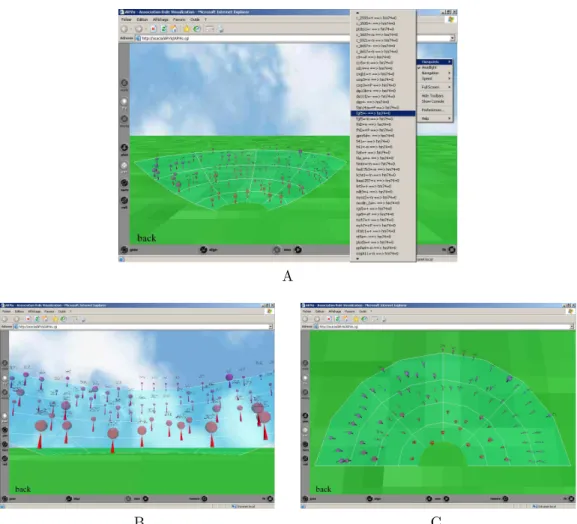
Each subset of rules is visualized in a 3D space, which we call a world. The representation is built in the following way: each rule is symbolized by an object composed of a sphere perched on top of a cone. Three straightforward graphical characteristics are thus obtained to represent the interestingness measures: the sphere diameter, the cone height, and the color. The representation size depends only on the number of rules in the subset and not on the amount of items. In order to facilitate the navigation (viewpoint control) inside the world, a ground and a sky are represented. As pointed out by Chen (2004), such visual landmarks make the navigation task easier by facilitating the acquisition of spatial knowledge, and more generally by facilitating the building of the cognitive map by the user (mental model of the world).
In a visual representation, the perceptually dominant information is the spa-tial position (Card et al., 1999). Therefore, in order to be emphasized, the inter-estingness measures which are fundamental for decision-making are represented by the object position in the world. Since several rules can present the same in-terestingness, only two measures can be symbolized by spatial position, so that the third dimension is free for scattering the objects. All things considered, we have chosen to use only one axis to place the objects in space and so to spatially represent only one interestingness measure. Indeed, the objects are laid out in the 3D world on an arena (a transparent half-bowl), which means that the fur-ther an object is, the higher it is placed (figure 7). This arena allows a better perception of the depth dimension and reduces occultation of objects by other objects. It can hold at most around 250 objects. A similar choice is made in the document manager Data Mountain of Microsoft Research, where web pages are laid out on an inclined plane (Robertson et al, 1998).
Weighing it all up, we have opted for the following visual metaphor to re-present each subset of rules by highlighting the interestingness measures (figure 8):
– the object position represents the entropic implication intensity,
– the sphere visible area represents the support,
– the cone height represents the confidence,
– the object color is used redundantly to represent a weighted average of confi-dence and entropic implication intensity, which gives a synthetic idea of the rule interestingness.
This visual metaphor facilitates comparisons among the rules. It stresses the good rules whose visualization and access are made easier compared to the less good
A
B C
Fig. 7.Each subset of rules is represented by a 3D world
A B
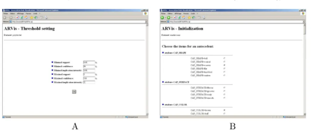
Fig. 9.Exploration initialization interface
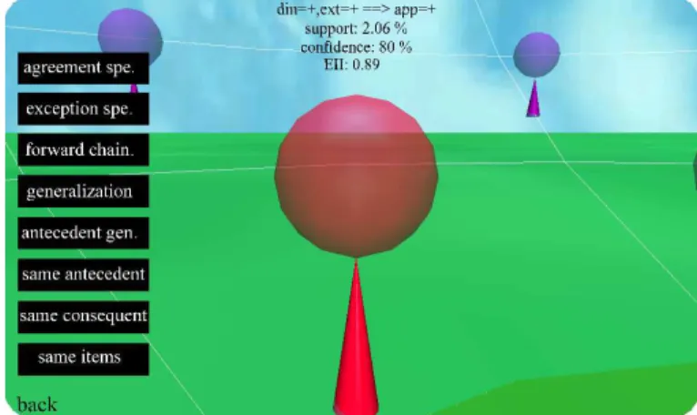
rules. More precisely, a large red sphere perched on top of a tall cone placed at the front of an arena, on the lower steps, represents a rule whose support, confidence and entropic implication intensity are high. On the other hand, a little blue sphere perched on top of a small cone placed at the back, on the upper steps, represents a rule whose three measures are weak. This metaphor is a choice among the many possible combinations. It can be adapted by the user. One can choose for instance to change the mappings, or to represent more interestingness measures with color or by using two axes for the spatial mapping. Furthermore, some complementary text labels appear above each object to give the name of the corresponding rule. They provide the numerical values for support, confidence and entropic implication intensity (noted ”EII”) too and thus complete the qualitative information given by the representation.
6.3. Interactions with the user
The user can interact in three different ways with the visual representation: by visiting a subset of rules, by filtering the rules on the interestingness measures in a subset, and by navigating among the subsets to discover new rules.
For each subset of rules, at the beginning of a visit, the user is placed in the 3D world in front of the arena so that (s)he benefits from an overall and synthetic view of the rules. With this comprehensive vision, it is easy to locate the best rules. Then the user can wander freely over the world to browse the rules, and zoom in on them to examine them more closely. (S)he just has to click on an object to move in front of it. In each 3D there also exist predefined viewpoints providing overall visions of the arena (cf. for instance, the viewpoint from the top in figure 7.C). If the user looks for a rule with particular items in it, (s)he can search it in a menu (figure 7.A) which lists all the rule names of the subset and allows to move directly in front of the object wanted. In the final analysis,ARVis enables the user to find the rules that interest him/her in a subset whether his/her search criteria are based on interestingness measures or on items.
At any time during the visit of a subset, the user can filter the rules on the interestingness measures by adjusting the thresholdsminsp,mincf, mineii,
Fig. 10. For each rule, a menu can be displayed to choose the neighborhood relation to be triggered
the thresholds are represented. This makes objects appear or disappear in the world.
Finally, the user can navigate among the subsets of rules via a menu providing the eight neighborhood relations (figure 10). By applying a neighborhood relation on a rule, the current subset is replaced by a new subset. Visually, the current world is replaced by a new world, which gives the impression of virtually moving inside the whole set of rules. At any time during the navigation, the user can go back to the previous subsets (and worlds) with the ”back” operator.
Let us assume that the user applies a neighborhood relation Π on a rule r. This generates a new subsetS= Π(r) containing all the rules neighbors ofr ac-cording to Π. InARVis, we systematically add the transitional rulerinto the new subsetS. Visually, the transitional rulercan be easily located in the world since its object flashes. This enables the user to make comparisons between the transi-tional rulerand its neighbor rules. For instance, with the neighborhood relation
agreement specialization, it is interesting to compare a rulerto its neighbors in order to see whether or not the addition of a new item inrtends to improve the rule interestingness. Reciprocally, with the relation generalization, comparing a ruler to its neighbors allows to detect the superfluous items inr(those whose removal does not reduce the quality of the rule).
To start or restart the navigation among the subsets, the user can choose the first subset to focus on with an exploration initialization interface (figure 9.B). This interface is an ”itemset browser” working with inclusive templates: it enables to build the itemset of one’s choosing and then to display the world of the rules that include this itemset in the antecedent, or in the consequent, or in both. Furthermore, the exploration initialization interface allows to choose the database and the table to be studied, and to choose the setIof the items to be used during the exploration.
6.4.
ARVis
implementation
6.4.1. Constraint-based rule-mining algorithm
When the user triggers a neighborhood relation,ARVis runs a constraint-based algorithm which dynamically computes the appropriate subset of rules with the interestingness measures. As seen in section 6.1, each of the eight neighborhood relations induces two kinds of constraints: syntactic constraints and interestin-gness measure constraints. These constraints are ”pushed” into association rule mining to reduce the exponentially growing search space. The general structure of the constraint-based algorithm is given below.
(1)ProcedureLocalMining
(2) Input: rule //the transitional rule (3) Π //the neighborhood relation
(4) thresholds //the 6 thresholds on interestingness measures (5) database //connection to the database
(6) Output:subsetrules,measures//subset of rules with interestingness measures
(7) subsetrules=∅ //subset of rules (without measures)
(8) cardinalities=∅ //cardinalities of the itemsets
(9) //STEP 1: Generate the candidate rules with the syntactic constraints (10) subsetrules= SyntacticGeneration(rule,Π)
(11) //STEP 2: Count the itemsets of the candidate rules (database scan) (12) cardinalities= RetrieveCardinalities(subsetrules,database)
(13) //STEP 3: Calculate the interestingness measures
(14) subsetrules,measures = CalculateMeasures(subsetrules,cardinalities)
(15) //STEP 4: Eliminate the candidate rules which do not respect (16) //the interestingness measure constraints
(17) subsetrules,measures = Filter(subsetrules,measures,thresholds)
(18) return(subsetrules,measures)
Only step 1 depends on the neighborhood relation Π chosen. This step needs no database scan since it deals only with the syntax of the rules. The syntac-tic constraints induced by the neighborhood relations of ARVis are powerful constraints which drastically reduce the number of rules to be produced. Effec-tively, the syntactic constraints are verified by at most |I| rules, whatever the relation chosen. It is easy to enumerate these candidate rules and therefore to enumerate all the itemsets that must be counted in the database during step 2 (Ng et al (1998) pointed out the interest of such itemset enumeration procedures in constraint-based itemset-mining). Thus, whatever the neighborhood relation chosen, the whole constraint-based algorithm has a polynomial complexity4 in O(|I|).
In this polynomial algorithm, the most time-consuming step is step 2. It consists in counting the cardinalities of the itemsets by scanning the database. To improve the response times of the algorithm, a progressive save system is
4 Except for the neighborhood relationexception specializationfor which the number of rules in a subset is bounded bym.|I|and the complexity is polynomial inO(m.|I|) wherem <|I|
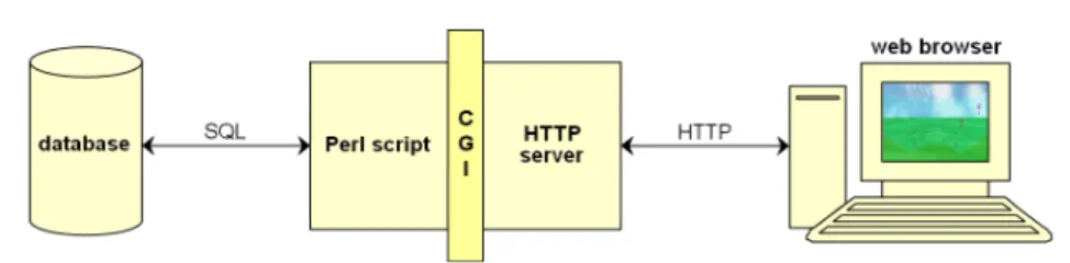
Fig. 11.ARVisarchitecture
implemented in the procedure RetrieveCardinalities: each time an itemset is counted, its cardinality is saved to avoid counting it another time during the remainder of the exploration. In this way, the greater number of times the algo-rithm is run over the same database, the more the itemset cardinalities are saved, and the more probable it is that the algorithm runs faster. The cardinalities of the itemsets are saved in the database in specific tables. There is one table for each itemset length (number of items in the itemset), so that all the itemsets of the same length are saved in the same table. For each table, the retrieval of the cardinalities uses a B-tree index.
Furthermore, for most of the neighborhood relations ofARVis, the constraint-based algorithm can be optimized by ”pushing” the interestingness measure constraints into step 1. With the progressive save system, one can indeed an-ticipate that some candidate rules do not respect the thresholds. Eliminating these candidate rules allows to reduce the number of itemsets that must be counted in the database during step 2. For example, with the neighborhood re-lationsame consequent, it is useless to generate a candidate rule antecedent→
consequentif the cardinality ofantecedenthas already been counted and does not respectcardinality≥n∗minsp/maxcf and cardinality≤n∗maxsp/mincf
wherenis the number of transactions in the database.
6.4.2. Architecture
ARVis is built on a client/server architecture with a thin client (figure 11). The main block is a CGI program in Perl divided into two parts:
– the constraint-based algorithm which dynamically extracts the subset of rules with their interestingness measures from the database,
– a procedure which dynamically generates the corresponding 3D world in VRML (this procedure is not time-consuming since no database access is needed). The user visits the worlds with a web browser equipped with a VRML plug-in. The exploration initialization interface is a series of web pages generated by the CGI program.
6.4.3. Response time
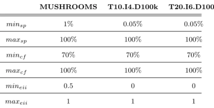
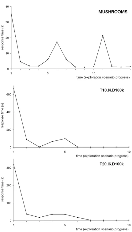
The figure 12 shows the response times obtained on three datasets (presented table 1) by executing an exploration scenario withARVis, i.e., a series of neighbo-rhood relations. For each relation triggered by the user, the response time is the time required byARVis to compute the subset of rules with the constraint-based algorithm and to display the corresponding world on the screen. The minimum and maximum thresholds chosen in the scenarios are given in table 2. For the
# of
items # oftransactions averagetransaction length
MUSHROOMS 119 8416 23
T10.I4.D100k 100 100000 10 T20.I6.D100k 40 100000 20
Table 1.Dataset characteristics
MUSHROOMS T10.I4.D100k T20.I6.D100k
minsp 1% 0.05% 0.05% maxsp 100% 100% 100% mincf 70% 70% 70% maxcf 100% 100% 100% mineii 0.5 0 0 maxeii 1 1 1
Table 2.Minimum and maximum thresholds used in the exploration scenarios
experiments, the server of ARVis was running on an SGI Origin 2000 server equipped with four 250 MHz RISC R10000 processors and with 512 MB of me-mory. The DBMS was PostgreSQL. The tables storing the itemset cardinalities were empty at the beginning of the scenarios.
The first dataset is the MUSHROOMS dataset from the UCI Repository (Blake and Merz, 1998). It is small but it is known to be highly correlated. The exploration scenario that was used with this dataset is given in table 3. The two other datasets are two large synthetic ones: T10.I4.D100k and T20.I6.D100k. They were generated by the procedure proposed by Agrawal and Srikant (1994) (the number of patterns was set to 1000). The dataset T20.I6.D100k is delibera-tely very dense (on average, each transaction contains 43 % of the items). The exploration scenarios for these two datasets are similar to the one given in the table 3 but we do not present them since the data have no real meaning.
As can be seen on figure 12, the response times tend to decrease as the scenario unfolds. This is due to the progressive save system of the constraint-based algorithm of ARVis. The peaks in the response time curve (for example for t=6 and t=11 in the MUSHROOMS scenario) appear when the algorithm needs lots of itemsets that have not been counted yet. In this case, like in any classical procedure for frequent itemset mining, the algorithm has to scan the database, which is time-consuming.
The experiment on the dataset T20.I6.D100k shows that ARVis can effi-ciently mine dense data. In particular, during this experiment, very specific rules containing up to 15 items and presenting a support of 0.07 % have been com-puted. With a levelwise exhaustive algorithm, such specific rules could never be extracted from a dense database.
Time Neigh b orho o d relation T ransitional rule (on whic h the neigh b orho o d relation is applied) Num b er of rules generated t=1 forwar d chaining C LAS S = edibl e → GI LL S I Z E = br oad 3 t=2 forwar d chaining C LAS S = edibl e, GI LL S I Z E = br oad → O D O R = none 4 t=3 same items C LAS S = edibl e, GI LL S I Z E = br oad, O D O R = none → S T ALK S H AP E = taper ing 3 t=4 ante ce dent gener alization GI LL S I Z E = br oad, O D O R = none, S T ALK S H AP E = taper ing → C LAS S = edibl e 3 t=5 same ante ce dent GI LL S I Z E = br oad, S T ALK S H AP E = taper ing → O D O R = none 7 t=6 same conse quent GI LL S I Z E = br oad, S T ALK S H AP E = taper ing → R I N G N U M B E R = one 54 t=7 forwar d chaining C LAS S = edibl e, GI LL S I Z E = br oad, S T ALK S H AP E = taper ing → O D O R = none 10 t=8 back + ante ce dent gener alization C LAS S = edibl e, GI LL S I Z E = br oad, S T ALK S H AP E = taper ing → O D O R = none 3 t=9 min cf = 60% + ante ce dent gener alization GI LL S I Z E = br oad, S T ALK S H AP E = taper ing → C LAS S = edibl e 2 t=10 forwar d chaining S T ALK S H AP E = taper ing → GI LL S I Z E = br oad 8 t=11 exc eption sp ecialization GI LL S I Z E = br oad, S T ALK S H AP E = taper ing → C LAS S = edibl e 4 t=12 forwar d chaining GI LL S I Z E = br oad → C LAS S = edibl e 3 t=13 forwar d chaining C LAS S = edibl e, GI LL S I Z E = br oad → O D O R = none 4 t=14 forwar d chaining C LAS S = edibl e, GI LL S I Z E = br oad, O D O R = none → S T ALK S H AP E = taper ing 10 T able 3. Exploration scenario for the MUSHR OOMS dataset
sta stability eas motivation for easiness fis fighting spirit pro motivation for protection ext extroversion rea motivation for realization que questioning mem motivation for membership
wil willpower pow motivation for power rec receptiveness imp improvisation
rig rigor dyn dynamism
inc intellectual conformism com communication anx anxiety aff affirmation soc spirit of conciliation ind independence
Table 4.Meaning of the attributes
7. Example of rule exploration with
ARVis
The example presented in this section comes from a case study made with the firm PerformanSe SA on human resource management data. The data are a set of workers’ psychological profiles used to calibrate decision support systems. It contains around 4000 individuals described by 20 categorical attributes (table 4). Each attribute has three possible values: ”+”, ”0”, and ”-”. In the example, since flashing objects cannot be seen on the figures, a transitional rule is represented in the worlds by an object with a white sphere.
The user begins by studying people that are extrovert and motivated by po-wer. By means of the exploration initialization interface, he displays the world that contains the rules with the itemset {ext=+, pow=+} in the antecedent (figure 13.A). The user explores the world. There are three rules with high confidence and high entropic implication intensity at the bottom of the arena, and one of them especially interests the user: {ext=+, pow=+} → {rec=−}. To know more characteristics of this not very receptive population, he applies the neighborhood relation forward chaining on this rule. The newly displayed world contains the rules with{ext=+, pow=+, rec=−}in the antecedent (figure 13.B). The user finds a rule which he thinks very pertinent: {ext=+, pow=+, rec=−} → {mem=+}. To know the other rules verified by these extrovert, not very receptive, and motivated by power and membership people, he applies the neighborhood relation same items on the rule. In the new world, the user sees the four rules that can be built with the four items (figure 13.C). One is the tran-sitional rule, two others are bad rules, and the fourth is a little better than the transitional rule: this is{ext=+, mem=+, rec=−} → {pow=+}. To know whe-ther all the items in the antecedent are useful in this rule, he applies the relation
generalization on it. In the new world (figure 13.D), there is the rule {ext=+, mem=+} → {pow=+}that is as good as the transitional rule, which means that the item {rec=−} was superfluous. Next, the user continues his exploration by examining the exceptions of the rule (figure 13.E).
For another exploration, the user is interested in rigorous people. He starts with the world containing the rules with{rig=+}in the antecedent (figure 14.A). His attention is drawn by the rule:{rig=+} → {anx=+}. This is quite a good rule, but he wants to verify whether other characteristics could better predict strong anxiety. To do so, he applies the neighborhood relationsame consequent. The new world contains the rules that conclude on {anx=+} and shows that there is no better rule than{rig=+} → {anx=+}(figure 14.B). So the user comes back to the previous world and applies the relationagreement specialization on
Fig. 14. An exploration withARVis
anxiety prediction. The new world presents some better rules effectively (figure 14.C).
8. Conclusion
In this article, we have presented the rule focusing methodology for the post-processing of association rules. It enables the user to explore large sets of rules freely by focusing his/her attention on interesting subsets. The methodology relies on:
– rule interestingness measures which filter and sort the rules,
– a visual representation which speeds up comprehension and makes the com-parisons among the rules easier,
– several neighborhood relations which connect the rules among them and un-derlie the interactive navigation among the rules.
We have also presented the prototype systemARVis which implements the rule focusing methodology by means of a 3D representation, of neighborhood re-lations meaningful for the user, and of a specific constraint-based rule-mining algorithm.ARVis takes advantage not only of the rule syntax, used in the neigh-borhood relations, but also of the interestingness measures, highlighted in the