Robust Signal Processing in Distributed Sensor Networks

Mark Ryan Leonard

Robust Signal Processing in Distributed Sensor Networks

Robust Signal Processing in

Distributed Sensor Networks

Dem Fachbereich

Elektrotechnik und Informationstechnik der Technischen Universität Darmstadt zur Erlangung des akademischen Grades eines

Doktor-Ingenieurs (Dr.-Ing.) vorgelegte Dissertation

von

Mark Ryan Leonard, M.Sc.

Erstgutachter: Prof. Dr.-Ing. Abdelhak M. Zoubir Zweitgutachter: Prof. Dr. Sergio Barbarossa

Jahr der Veröffentlichung der Dissertation auf TUprints: 2019 URN: urn:nbn:de:tuda-tuprints-84896

Tag der mündlichen Prüfung: 15. Februar 2019

Veröffentlicht unter CC BY-NC-SA 4.0 International

“Start every week with a break-neck urgent design

And end every speed day with my briefcase representing free time Spending my fruit as my purchases become my lifeline

Please give my love to my family I’ll doubtfully be home at christmas time

Don’t disturb me in this state Please leave me purgatorying I’ll be damned if I’m to wake This is far more than I am equipped for.” Alanis Morissette – Purgatorying

F 6 f

To Bennett

F 6 f

“Flowers are more beautiful than they are thirty-eight.” Oren Lavie – The Bear Who Wasn’t There

Acknowledgments

I wish to thank everyone, who contributed to this thesis in various ways and supported me during this truly transformative time of my life.

First of all, I would like to thank Prof. Dr.-Ing. Abdelhak M. Zoubir for giving me the op-portunity to pursue my Ph.D. at the Signal Processing Group. Thank you for your continued guidance and support, your understanding, and for all the freedom that allowed me to perse-vere and finish this project in the first place.

Thanks to Prof. Dr. Sergio Barbarossa for being my co-advisor. I really appreciated your valuable comments on my work. I also wish to thank Prof. Dr.-Ing. Rolf Jakoby and Prof. Dr.-Ing. Anja Klein for making my defense as pleasurable as an exam can be.

I sincerely want to thank Renate Koschella for everything you have done and continue to do for me and the entire group. Thank you for your compassion and support and the countless encouraging, calming, and liberating talks over the years. I am certain that a lot of doctoral candidacies would have ended differently if it weren’t for you.

Big thanks go to Dr.-Ing. Michael Fauß. Thank you for your guidance and for always help-ing me whenever I was stuck. Also, thanks for proof-readhelp-ing virtually all of my publications— including this thesis—and for finding even the most unspottable errors.

I also wish to thank my various roommates over the years, starting with Dr.-Ing. Stefan Leier. Thank you for your clear words although I wouldn’t listen. Thank you Dr.-Ing. Nevine Demitri for helping me turn our office into the best coffee shop in town. Thank you to Di Jin for transforming it into the best tea house in the western hemisphere. Dominik Reinhard, thank you for all the sarcastic comments, which made even bad times more endurable. Also thanks for helping me in keeping the office well-ventilated at all times.

Thank you to my partner in crime Freweyni Kidane Teklehaymanot for finishing this to-gether. Also, thanks for the wonderful times in Calgary and Rome. I’ll never forget the great vegan food we had and how we discovered the entryway to the underworld. And you should always remember the secret ;)

Thanks to Dr.-Ing. Lala Khadidja Hamaidi. Merci beaucoup de me tenir compagnie dans la contrée sauvage.

Thank you Dr.-Ing. Sahar Khawatmi for your cheerful nature and all the fun we had trying to figure out German grammar.

Thanks to Hauke Fath for always trying your best in making our system work.

I would like to thank all of my other current and former colleagues and members of the group, including Dr.-Ing. Sara Al-Sayed, Dr.-Ing. Mouhammad Alhumaidi, Patricia Binder, Jack Dagdagan, Dr.-Ing. Christian Debes, Dr.-Ing. Tai Fei, Dr. Stefano Fortunati, Dr.-Ing.

Gök-fik Mouchini, Dr.-Ing. Michael Muma, Afief Dias Pambudi, Prof. Dr.-Ing. Henning Puder, Ziliang Qiao, Ing. Simon Rosenkranz, Ing. Tim Schäck, Ann-Kathrin Seifert, Ing. Adrian Šošić, Sergey Sukhanov, Ing. Wassim Suleiman, Ing. Fiky Suratman, Dr.-Ing. Christian Weiss, Dr.-Dr.-Ing. Feng Yin, and Dr.-Dr.-Ing. Wenjun Zeng. You made these last five years very enjoyable.

Thank you Roman Hocke for giving me the opportunity to pursue my other passion dur-ing these past five years—and for half of my life. Thanks to Lisa Blenndur-inger, Claudia von Hornstein, Markus Michalek and Dr. Cornelia Petersen-Laux for the great collaboration over all these years.

Special thanks go to Sabine Schmelzer for fixing me up and to Salima Elyazidi for always finding time for that.

Finally I would like to thank my family. Thanks to my parents Gerhard and Renate, my sister Jennifer, and my mother-in-law Monika for your unconditional love and support and for always believing in me. Thank you Jonathan, Tineke, and Hugo for providing the best and most relaxing seaside getaways one could wish for. Thanks to Fee, Lotta, Lotti, Mäxchen, Merle, Samson, and Sissi for all the joy and consolation.

Thank you René for these intense last three months, a wonderful Christmas eve, and for holding out until after my defense. You will be missed very much.

Thank you to my wife Fabienne. Thank you for all that you are, all that you made me, and all that we will become.

Mark Ryan Leonard 04. Dezember 2018

Robuste Signalverarbeitung

in verteilten Sensornetzen

Kurzfassung

Statistische Robustheit und kollaborative Inferenz in einem verteilten Sensornetz sind zwei anspruchsvolle Herausforderungen, die an viele moderne Signalverarbeitungsanwendungen gestellt werden. Diese Dissertation hat zum Ziel, gemeinsame Lösungen für diese Aufgaben zu entwickeln und generische Algorithmen bereitzustellen, die auf eine Vielzahl von Proble-men aus der Praxis anwendbar sind.

Der erste Teil der Arbeit befasst sich mit der sequentiellen Detektion – einem Teilgebiet der Detektionstheorie, das sich auf die Entscheidungsfindung basierend auf einer möglichst geringen Anzahl von Messwerten konzentriert. Nach der Betrachtung einiger grundlegen-der Konzepte des statistischen Hypothesentests wird eine allgemeine Formulierung des se-quentiellen Konsens+Innovationen Likelihood-Quotienten-Tests (Consensus+Innovations Sequential Probability Ratio Tests) zum sequentiellen Testen binärer Hypothesen in verteil-ten Netzen hergeleitet. In einem nächsverteil-ten Schritt werden mehrere robuste Versionen des Algorithmus’ entwickelt, die auf zwei verschiedenen Robustheitsparadigmen basieren. Die Funktionalität der vorgestellten Detektoren wird in Simulationen verifiziert und ihre Leis-tung wird unter verschiedenen Netzwerkbedingungen sowie Ausreißerkonzentrationen un-tersucht. Anschließend wird das Konzept auf mehrere Hypothesen ausgedehnt, indem es mit dem sequentiellen Matrix-Likelihood-Quotienten-Test (Matrix Sequential Probability Ratio Test) fusioniert wird. Ferner werden robuste Versionen des resultierenden Algorithmus’ ent-wickelt. Die Leistungsfähigkeit der vorgeschlagenen Algorithmen wird in Simulationen ve-rifiziert und evaluiert. Schließlich wird die Dempster-Shafer Evidenztheorie erstmals in der Literatur auf verteilte sequentielle Hypothesentests angewendet. Nach der Vorstellung einer neuartigen Methode für die Zuweisung von Wahrscheinlichkeitsmassen (Basic Probability As-signment) wird ein evidenzbasierter sequentieller Detektor für den Einsatz in verteilten Sen-sornetzen entwickelt und seine Leistungsfähigkeit in Simulationen verifiziert.

Der zweite Teil der Dissertation beschäftigt sich mit der Mehrziel-Verfolgung in verteil-ten Sensornetzen. Das Problem der Daverteil-tenzuordnung wird diskutiert und die betrachteverteil-ten Zustandsraum- und Messmodelle werden eingeführt. Als Nächstes werden das Konzept der zufälligen endlichen Mengen sowie die Wahrscheinlichkeitshypothesendichte-Filterung (Prob-ability Hypothesis Density Filtering) beleuchtet. Anschließend wird eine neuartige verteilte Partikel-Filter Implementierung des Wahrscheinlichkeitshypothesendichte-Filters entwickelt, die auf einem zweistufigen Kommunikationsschema basiert. Es wird sowohl eine robuste als

auch eine zentralisierte Version des Algorithmus’ hergeleitet. Darüber hinaus werden Rechen-komplexität und Kommunikationslast des verteilten sowie des zentralen Verfolgungsalgorith-mus’ analysiert. Schließlich werden Simulationen durchgeführt, in denen die vorgeschlage-nen Methoden mit einem existierenden verteilten Verfolgungsalgorithmus verglichen werden. Zu diesem Zweck wird eine verteilte Version der A-posteriori-Cramér-Rao-Schranke (Poste-rior Cramér-Rao Lower Bound) entwickelt, die als Leistungsgrenze dient. Die Ergebnisse zeigen, dass die vorgestellten Algorithmen unter verschiedenen Umgebungsbedingungen gut funktionieren und die Konkurrenz übertreffen.

Mark Ryan Leonard December 04, 2018

Robust Signal Processing in

Distributed Sensor Networks

Abstract

Statistical robustness and collaborative inference in a distributed sensor network are two challenging requirements posed on many modern signal processing applications. This disser-tation aims at solving these tasks jointly by providing generic algorithms that are applicable to a wide variety of real-world problems.

The first part of the thesis is concerned with sequential detection—a branch of detection theory that is focused on decision-making based on as few measurements as possible. After re-viewing some fundamental concepts of statistical hypothesis testing, a general formulation of the Consensus+Innovations Sequential Probability Ratio Test for sequential binary hypoth-esis testing in distributed networks is derived. In a next step, multiple robust versions of the algorithm based on two different robustification paradigms are developed. The functional-ity of the proposed detectors is verified in simulations, and their performance is examined under different network conditions and outlier concentrations. Subsequently, the concept is extended to multiple hypotheses by fusing it with the Matrix Sequential Probability Ratio Test, and robust versions of the resulting algorithm are developed. The performance of the proposed algorithms is verified and evaluated in simulations. Finally, the Dempster-Shafer Theory of Evidence is applied to distributed sequential hypothesis testing for the first time in the literature. After introducing a novel way of performing the basic probability assign-ment, an evidence-based sequential detector for application in distributed sensor networks is developed and its performance is verified in simulations.

The second part of the thesis deals with multi-target tracking in distributed sensor net-works. The problem of data association is discussed and the considered state-space and mea-surement models are introduced. Next, the concept of random finite sets as well as Probabili-ty Hypothesis DensiProbabili-ty filtering are reviewed. Subsequently, a novel distributed Particle Filter implementation of the Probability Hypothesis Density Filter is developed, which is based on a two-step communication scheme. A robust as well as a centralized version of the algorithm are derived. Furthermore, the computational complexity and communication load of the dis-tributed as well as the centralized trackers are analyzed. Finally, simulations are performed to compare the proposed algorithms with an existing distributed tracker. To this end, a dis-tributed version of the Posterior Cramér-Rao Lower Bound is developed, which serves as a performance bound. The results show that the proposed algorithms perform well under dif-ferent environmental conditions and outperform the competition.

Publications

The following publications have been produced during the period of doctoral candidacy.

I n t e r n at i o n a l ly R e f e r e e d J o u r n a l A rt i c l e s

M. R. Leonard&A. M. Zoubir. “Multi-Target Tracking in Distributed Sensor Networks using Particle PHD Filters.” In:Signal Processing159 (June 2019), pp. 130–146.

M. R. Leonard&A. M. Zoubir. “Robust Sequential Detection in Distributed Sensor Net-works.” In:IEEE Transactions on Signal Processing66.21 (Nov. 2018), pp. 5648–5662.

I n t e r n at i o n a l ly R e f e r e e d C o n f e r e n c e P a p e rs

M. R. Leonard, M. Stiefel, M. Fauß&A. M. Zoubir. “Robustifying Sequential Multiple Hypothesis Tests in Distributed Sensor Networks.” In:Proceedings of the 26th European Signal Processing Conference (EUSIPCO). Sept. 2018.

M. R. Leonard, C. A. Schroth &A. M. Zoubir. “Dempster-Shafer Theory Based Robust Sequential Detection in Distributed Sensor Networks.” In:Proceedings of the IEEE Sta-tistical Signal Processing Workshop (SSP). June 2018.

M. R. Leonard, M. Stiefel, M. Fauß&A. M. Zoubir. “Robust Sequential Testing of Multiple Hypotheses in Distributed Sensor Networks.” In:Proceedings of the 43nd IEEE Interna-tional Conference on Acoustics, Speech and Signal Processing (ICASSP). Mar. 2018. M. R. Leonard&A. M. Zoubir. “Robust Distributed Sequential Hypothesis Testing for

Detecting a Random Signal in Non-Gaussian Noise.” In:Proceedings of the 25th European Signal Processing Conference (EUSIPCO). Sept. 2017.

W. Hou, M. R. Leonard& A. M. Zoubir. “Robust Distributed Sequential Detection via Robust Estimation.” In: Proceedings of the 25th European Signal Processing Conference (EUSIPCO). Sept. 2017.

Face Recognition and Tracking.” In:Proceedings of the 12th IEEE International Confer-ence on Advanced Video and Signal Based Surveillance (AVSS). Aug. 2015.

I n t e r n at i o n a l C o n f e r e n c e P a p e rs

M. R. Balthasar, S. Al-Sayed, S. Leier & A. M. Zoubir. “Optimal Area Coverage in Au-tonomous Sensor Networks.” In: Proceedings of the 2nd International Conference and Exhibition on Underwater Acoustics (UA2014). Invited Paper. June 2014.

F i l e d P at e n t A p p l i c at i o n s

J. Rambach, M. Huber&M. R. Balthasar. “Method Of Distributed Face Recognition And System Thereof.” Patent Application WO 2017/125915 A1 (World Intellectual Property Or-ganization). July 27, 2017.

J. Rambach, M. Huber&M. R. Balthasar. “Method Of Distributed Face Recognition And System Thereof.” Patent Application US 2017/0206403 A1 (United States). July 20, 2017.

Contents

1 Introduction 1

1.1 Sequential Detection . . . 2

1.2 Location Estimation&Tracking . . . 3

1.3 Overview&Contributions . . . 3

2 Fundamentals 7

2.1 Statistical Robustness . . . 7

2.2 Distributed Sensor Networks . . . 10

Part I:

Sequential Detection

3 Statistical Hypothesis Testing 17

3.1 Fixed-Sample-Size Hypothesis Testing . . . 17

3.2 Sequential Hypothesis Testing . . . 20

3.3 Least Favorable Densities . . . 22

4 Robust Sequential Binary Hypothesis Testing 25

4.1 Problem Formulation . . . 26

4.2 The Consensus+Innovations Sequential Probability Ratio Test . . . 27

4.3 Decision Thresholds for theCISPRT . . . 28

4.4 A Robust Version of theCISPRT Based on Least Favorable Densities . . 35

4.5 Robust Versions of theCISPRT Based on Robust Estimators . . . 39

4.6 Simulations . . . 42

4.7 Summary . . . 49

5 Robust Sequential Multiple Hypothesis Testing 51

5.1 Problem Formulation . . . 52

5.2 The Matrix Sequential Probability Ratio Test . . . 52

5.4 Expected Runlength of theCIMSPRT . . . 54

5.5 Robust Versions of theCIMSPRT . . . 54

5.6 Simulations . . . 55

5.7 Summary . . . 63

6 Evidence-Based Sequential Hypothesis Testing 65 6.1 The Dempster-Shafer Theory of Evidence . . . 66

6.2 Evidence-Based Distributed Sequential Detection . . . 69

6.3 Simulations . . . 74

6.4 Summary . . . 76

7 Conclusions&Outlook 77 7.1 Arbitrary Sequential Hypothesis Tests . . . 78

7.2 Analysis of the Impact of Network Properties . . . 78

7.3 Heterogeneous Sensor Networks . . . 78

Part II: Location Estimation

&

Tracking

8.2 State-Space and Measurement Model . . . 84

8.3 Random Finite Sets . . . 86

8.4 The Probability Hypothesis Density . . . 87

8.5 The Probability Hypothesis Density Filter . . . 89

9 Distributed Multi-Target Tracking 91 9.1 Adaptive Target Birth . . . 92

9.2 The Diffusion Particle PHD Filter . . . 93

9.3 Computational Complexity and Communication Load . . . 99

9.4 Robust Versions of the Diffusion Particle PHD Filter . . . 100

10 Centralized Multi-Target Tracking 103 10.1 The Multi-Sensor Particle PHD Filter . . . 103

C o n t e n t s

11 Performance Evaluation 109

11.1 The Optimal Subpattern Assignment Metric . . . 110

11.2 The Distributed Posterior Cramér-Rao Lower Bound . . . 110

11.3 Simulations . . . 112

11.4 Summary . . . 122

12 Conclusions&Outlook 123 12.1 More Sophisticated Tracking Scenarios . . . 123

12.2 A Multi-Sensor Probability Hypothesis Density . . . 124

Part III: Appendix

A.2 Decision Thresholds for theCISPRT . . . 132

B Appendix to Part II 135 B.1 Pseudo-Code of the Diffusion Particle PHD Filter . . . 135

B.2 Pseudo-Code of the Multi-Sensor Particle PHD Filter . . . 137

List of Abbreviations&Acronyms 139

List of Figures 141

List of Notations&Symbols 143

1

Introduction

An increasing number of modern signal processing applications have to prevail under two fundamental circumstances: On the one hand, non-Gaussian disturbances such as impulsive noise call for robust solutions that accomplish the balancing act between optimality under nominal conditions and reliability in the face of distributional uncertainties [Huber, 1964;Huber, 1965;Huber&Strassen, 1973;Huber, 1981;Levy, 2008;Zoubir et al., 2012;Gül

&Zoubir, 2017a;Zoubir et al., 2018]. On the other hand, the growing tendency to network ever more capable sensors and devices demands fully distributed architectures that do away with error-prone and communication-intensive central processing units [Cattivelli&Sayed, 2011; Tu&Sayed, 2011; Sayed, 2013;Balthasar et al., 2014; Leonard&Zoubir, 2019; Matta et al., 2016]. The dissertation at hand is focused on jointly solving these problems for a wide variety of real-world applications—whether it be air and ground traffic control, climate or health monitoring, smart homes and cities, or video surveillance [Tartakovsky et al., 2014]. To this end, generic algorithms are derived that can be easily deployed in distributed network architectures. Furthermore, a balance is struck between approximating the performance of centralized solutions and providing resilience in the face of unknown disturbances, all the while accounting for resource constraints at the individual network agents.

The aforementioned real-world applications and many others are based on two consecu-tive steps that are elementary to statistical signal processing: thedetectionof a phenomenon, and the subsequentestimation—and possibly tracking—of relevant parameters. While, in the first step, it is imperative to register new phenomena and parameter shifts instantly, step two requires continuous, accurate estimates and predictions of the parameters of interest. A sepa-rate part is dedicated to each of these two steps.

1 . 1

S e q u e n t i a l D e t e c t i o n

The first part of the thesis is concerned with a particular branch of detection theory: sequen-tial detection [Wald, 1945;Wald, 1947;Novikov, 2009a;Novikov, 2009b;Tartakovsky et al., 2014;Fauß&Zoubir, 2015;Fauß, 2016]. While originally introduced in the 1940s by Wald, sequential hypothesis testing has been gaining traction recently as a growing number of ap-plications require accurate decision-making in a timely manner. The objective is to make a reliable decision for one out of two or more hypotheses based on as few measurements as pos-sible, which can reduce the testing time by up to50%on average. To this end, a test statistic is continually updated as new samples are taken, and the threshold comparisons are repeated until the gathered information warrants an accurate decision with respect to a specified confi-dence measure.

Robustness, sequentiality, and a distributed network architecture are challenging, partially contradictory requirements to pose on a statistical hypothesis test. While combinations of either two of them—i.e., distributed sequential detection [Teneketzis&Ho, 1987;Blum et al., 1997;Sahu&Kar, 2014;Sahu&Kar, 2016;Liu&Mei, 2017;Li&Wang, 2018], robust sequential detection [DeGroot, 1960;Schmitz, 1987;Fauß&Zoubir, 2016; Gül&Zoubir, 2017a], and robust hypothesis testing in distributed sensor networks [Veeravalli et al., 1994;

Blum et al., 1997;Gül, 2017;Gül&Zoubir, 2017b;Al-Sayed et al., 2017]—have received con-siderable attention in recent years, their complete union has not been treated in the literature, yet.

1 . 2 L o c a t i o n E s t i m a t i o n& Tr a c k i n g

1 . 2

L o c at i o n E s t i m at i o n

&

Tr a c k i n g

The second part of the thesis considers the problem of estimating and tracking the location of multiple targets at once with the help of a distributed sensor network. This task is becom-ing increasbecom-ingly relevant in many military and civilian applications includbecom-ing air and ground traffic control, harbor surveillance, maritime traffic control, and video communication and surveillance [Challa et al., 2011;Maresca et al., 2014;Rambach et al., 2015].

A distributed network architecture offers several properties that make it desirable for track-ing applications in general [Olfati-Saber et al., 2007]. The state-of-the-art of distributed single-targettracking is well summarized in [Hlinka et al., 2013]. Distributed versions of the Kalman Filter [Hlinka et al., 2013;Cattivelli et al., 2008] and the Particle Filter [Arulampalam et al., 2002] suffer from the problem of data association and cannnot be applied directly to multi-target tracking. Methods like the Joint Probabilistic Data Association Filter [Bar-Shalom et al., 2011] or the Multiple Hypothesis Tracker [Reid, 1979] address this problem in the single-target case but the resource constraints arising in sensor networks pose a challenge on the development of distributed implementations thereof [Oh et al., 2007].

The algorithms considered in the dissertation at hand are based on the concept of Probabi-lity Hypothesis Density (PHD) filtering [Mahler, 2003;Clark, 2006], which circumvents the data association issue by modeling the tracking problem with the help of random finite sets. Furthermore, the focus is on sensor networks with maximum area coverage and neighborhood communication. Other solutions based on thePHDFilter have been studied, e.g., in [Uney et al., 2010;Uney et al., 2013; Battistelli et al., 2013]. Contrary to the methods presented in this work, these approaches either assume overlapping fields of view or employ a pairwise communication scheme. The common idea, however, is to extend the single-sensorPHD

Filter to the multi-sensor case through communication between multiple nodes, or nodes and a fusion center.

1 . 3

O v e rv i e w

&

C o n t r i b u t i o n s

The dissertation is divided into two parts. Before diving into each of them,Chapter 2gives an overview of the fundamental concepts used throughout the thesis—statistical robustness and distributed sensor networks.

P a rt I : S e q u e n t i a l D e t e c t i o n

The first part investigates robust sequential hypothesis testing in distributed sensor networks with the goal of obtaining a networkwide decision on the considered phenomenon. In Chap-ter 3, the basics of fixed-sample-size hypothesis testing, sequential hypothesis testing, and least favorable densities (LFDs) are reviewed.

Chapter 4is concerned with sequential binary hypothesis tests in distributed sensor net-works. Here, a general formulation of the Consensus+Innovations Sequential Probability Ratio Test (CISPRT)—originally introduced in [Sahu&Kar, 2014;Sahu&Kar, 2016]— is derived, which is not only applicable to arbitrary binary hypothesis tests but also suitable for real-world distributed detection problems. Furthermore, multiple robust versions of the

CISPRTare developed based on two different robustification paradigms, namely,LFDsand robust estimators. Finally, the proposed algorithms are evaluated in simulated shift-in-mean and shift-in-variance tests.

The problem of sequentially testing multiple hypotheses in a distributed network architec-ture is the topic ofChapter 5. First, the Matrix Sequential Probability Ratio Test (MSPRT) for testing multiple hypotheses in a centralized setup is reviewed. Afterwards, the Consensus+In-novations Matrix Sequential Probability Ratio Test (CIMSPRT) is proposed as a fusion of theCISPRTand theMSPRT. Furthermore, it is shown how the expected runlength of the algorithm can be accurately approximated. In a next step, robust versions of theCISPRT

are developed based onLFDsand robust estimators. The performance of the proposed algo-rithms is verified and evaluated in the simulation section.

Chapter 6considers the alternative paradigm of evidence-based hypothesis testing in a se-quential and distributed manner. After formulating the problem, an overview of the Demp-ster-Shafer Theory of Evidence (DST) is given. Subsequently, a distributed sequential detec-tor based on this theory is proposed, which uses a novel approach for performing the basic probability assignment (BPA). Furthermore, methods for robustifying the algorithm against outliers are presented. The performance of the proposed methods is validated and evaluated through simulations.

Chapter 7draws conclusions and provides an outlook into possible future research direc-tions.

1 . 3 O v e r v i e w& C o n t r i b u t i o n s P a rt I I : L o c at i o n E s t i m at i o n & Tr ac k i n g

The second part of this work is concerned with the estimation and subsequent tracking of location parameters in the example of distributed multi-target tracking.

Chapter 8provides an introduction into the problem of multi-target tracking. First, the data association issue is discussed. Subsequently, the considered state-space and measurement models are introduced and a review of the theory behind random finite sets is given. Finally, an overview of thePHDand thePHDFilter is provided.

InChapter 9, a novel distributed multi-tracking algorithm based on ParticlePHD filter-ing—the Diffusion Particle PHD Filter (D-PPHDF)—is proposed and its computational complexity as well as its communication load are analyzed. Furthermore, a method for ro-bustifying theD-PPHDFbased on robust estimators is introduced and two robust variants are developed.

A centralized version of theD-PPHDFtracker—the Multi-Sensor Particle Probability Hy-pothesis Density Filter (MS-PPHDF)—is developed inChapter 10. Again, an analysis of its computational complexity and communication load is performed.

Chapter 11is dedicated to the performance evaluation of the proposed tracking algorithms. Simulations are run to compare them to an existing distributed tracker in different Gaussian and non-Gaussian environments. Furthermore, a distributed version of the Posterior Cramér-Rao Lower Bound (PCRLB) is derived that serves as a performance benchmark.

2

Fundamentals

The two overarching themes of this work are statistical robustness and distributed sensor networks. The purpose of this chapter is to give a brief overview of both of these topics and introduce important notions and concepts needed in the two major parts of the thesis.

2 . 1

S t a t i s t i c a l R o b u s t n e s s

Statistical robustness is an area of statistics that deals with deviations from distributional as-sumptions. While the assumption of a Gaussian noise environment simplifies the derivation of optimal detectors and estimators, this premise is violated in many practical applications. In this case, even slight deviations from the assumptions—e.g., in the form of outlying measure-ments—are enough to cause a performance degradation or even the breakdown of a nomi-nally optimal algorithm. The aim of robust signal processing is to account for distributional uncertainties by developing algorithms that exhibit a close-to-optimal performance while tol-erating a certain degree of deviation from the assumptions made. Further details on statistical robustness can be found in [Zoubir et al., 2012;Zoubir et al., 2018] and the references therein.

three robust estimators of location are presented. These estimators are used in the design of robust detection and tracking algorithms inPart IandPart II, respectively.

2 . 1 . 1 ε- co n ta m i n at e d N o i s e

A popular way to model measurement outliers isε-contamination. Here, a fraction of the measurement set is assumed to be drawn from a contamination distributionHsuch that

P = (1−ε)P◦+εH,

where0 ≤ ε < 0.5is the contamination factor andP◦ denotes the nominal distribution. The corresponding probability density function (PDF) reads as

p= (1−ε)p◦+εh.

In this work, the nominal distribution is considered to be Gaussian with meanµand variance σ2, i.e.,

P◦ =N(µ, σ2).

Furthermore, the focus is on Gaussian contamination distributions with the same mean but

aκ-times higher variance, i.e.,

H =N(µ, κσ2).

2 . 1 . 2 Th e S a m p l e M e d i a n

Thesample meancalculates the arithmetic average of a data setM={x1, x2, . . .}according

to ˆ xmean= 1 |M| |M| ∑ i=1 xi.

Hence, a single outlier is enough to cause a significant deviation from the expected value of the uncontaminated data set [Zoubir et al., 2012]. The sample mean is, therefore, a non-robust

2 . 1 S t a t i s t i c a l R o b u s t n e s s

location estimator.

A simple alternative to the sample mean is thesample median, which returns the middle value of the sorted data set. Therefore, it can handle up to50 %outliers before breaking down. Withxdenoting the ordered vector of observations, the sample median reads as

ˆ xmedian=      x ( |M|+1 2 ) , |M|odd, 1 2 ( x ( |M| 2 ) +x ( |M| 2 + 1 )) , |M|even. (2.1) 2 . 1 . 3 Th e M - e s t i m ato r

M-estimators are an important class of robust estimators [Huber, 1981; Zoubir et al., 2012;

Zoubir et al., 2018]. Intuitively speaking, M-estimators of location provide a weighted average of the input data with weights given by

W(x) =    ψ(x) x , x̸= 0, ψ′(0), x= 0,

whereψ(x)is a score function andψ′(x)its first derivative. The purpose of the score func-tion is to downweight the influence of outliers while weighting the meaningful data close to one. Hence, an appropriate choice ofψ(x)is key in designing a robust estimator with high efficiency in the nominal case. While there is a variety of viable score functions*_{, this work}

focuses on Huber’s score function, which is defined as

ψHub(x) =    x, |x| ≤cHub, cHubsign(x), |x|> cHub, for some positive constantcHub.

*_{As a matter of fact, the sample median and the sample myriad can both be formulated as M-estimators by}

The M-estimate of the input data is obtained by recursively calculating wi(k) =W ( xi−xˆM(k) ˆ σ(x) ) , ˆ xM(k+ 1) = ∑_|M| i=1 wi(k)xi ∑_|M| i=1wi(k) ,

until |xˆM(k+1)_σˆ(x−₎xˆM(k)| < ϵ for a small, positive constantϵ. The algorithm is initialized by settingxˆM_{(0) = ˆx}median_{and estimating the scale using the normalized median standard} deviation according to

ˆ

σ_mad(x) = 1.483·median(|x−xˆmedian|), where the median is calculated as in(2.1).

2 . 1 . 4 Th e S a m p l e M y r i a d

The sample myriad is a type of M-estimator derived from optimality criteria in the Cauchy dis-tribution. Compared to the Gaussian distribution, the Cauchy distribution has much heavier tails. Hence, when sampling from this distribution, the probability of drawing very large val-ues is non-negligible—i.e., outliers can occur.

The sample myriad of ordermreads as

ˆ

xmyriad = arg min

x |M| ∏ i=1 [ m2+ (xi−x) 2] ,

wheremis a freely tunable parameter commonly set tom= ˆσ_mad(x). Further details about this type of M-estimator can be found in [Gonzalez&Arce, 1996;Gonzalez&Arce, 2002].

2 . 2

D i s t r i b u t e d S e n s o r N e t w o r k s

A network of multiple agents or nodes can be categorized into one of three architectures: cen-tralized, decencen-tralized, or distributed [Akyildiz et al., 2002;Karl&Willig, 2007]. In a cen-tralized sensor networkthere is a central processing unit calledfusion center, which typically

2 . 2 D i s t r i b u t e d S e n s o r N e t w o r k s

collects the raw data observed at the individual agents to perform the signal processing task at hand. Ultimately, the final result is broadcast back to the agents. In such a network the agents either communicate directly with the fusion center or the data is relayed via neighbor-ing agents. Networks of this kind suffer from the fact that the fusion center poses a sneighbor-ingle point of failure.

Decentralized sensor networks(see, e.g., [Veeravalli et al., 1993;Veeravalli, 1999]) share most of the properties of centralized sensor networks. The key difference is that the agents per-form some if not all processing locally, either based entirely on their own measurements or through local interactions with their neighbors. The final decision or data fusion, however, is performed at the fusion center, which broadcasts the global result back to the agents.

Indistributed sensor networks (see, e.g., [Sahu&Kar, 2016;Leonard&Zoubir, 2018a]) the individual nodes have enough communication and processing capabilities to perform the signal processing task entirely through local interactions with their neighbors. Since no fu-sion center is involved, there is no single point of failure. Furthermore, these networks are inherently redundant and fault-tolerant such that the loss of a single agent can easily be com-pensated [Olfati-Saber et al., 2007]. Moreover, the individual sensors are typically low-cost and can be easily deployed. In order to converge to the same global result at each agent, how-ever, consensus-like algorithms are needed. Furthermore, the communication load emerging from such a setup has to be kept at bay.

A distributed sensor network ofNagents or nodes can be modeled as a graphG = (V,E) withV denoting the set of agents andE being the set of edges between these agents. The graph issimple—i.e., devoid of self-loops—,undirected—i.e., if nodekis connected to node l, the reverse is also true—, andconnected—meaning that no separate subgraphs exist. The openneighborhood of agentkis defined as

No

k ={l∈ V | (k, l)∈ E},

i.e., the set of all agents to whichkis connected by an edge. When agentkitself is included in the set, one speaks of theclosedneighborhood, which is given by

A simple way to define the open neighborhood of nodekis by means of thedisc model ac-cording to

No

k ={l ∈ V | ∥xk−xl∥ ≤rcom},

where∥·∥is the Euclidean distance andxkdenotes the location vector of nodek. This

defini-tion is useful in many applicadefini-tions where data is broadcast and errors due to the degradadefini-tion of signal strength with distance are neglected. In words, the open neighborhood of nodek is defined by a communication radiusr_comaround its location. The closed neighborhood is again obtained as in(2.2).

Part I

3

Statistical Hypothesis Testing

Target detection in radar, spectrum sensing in cognitive radio, and object detection in image processing are just a few examples for detection problems that can be cast as statisti-cal hypothesis tests. This chapter gives a brief overview of fixed-sample-size hypothesis tests inSection 3.1, sequential hypothesis tests inSection 3.2, as well as the concept of least favor-able densities (LFDs) inSection 3.3, and introduces common notions needed in the follow-ing chapters. Details on fixed-sample-size tests can be found, e.g., in [Van Trees, 2004;Levy, 2008;Poor, 2013]. Further information on sequential hypothesis testing in general and the Sequential Probability Ratio Test (SPRT) in particular is given in [Wald, 1947]. The concept ofLFDsis explained in [Fauß&Zoubir, 2016].

3 . 1

F i x e d - S a m p l e - S i z e H y p o t h e s i s Te s t i n g

The goal of fixed-sample-size hypothesis testing is to make a statement about some prevalent phenomenon based on a random vectorY = [Y1, . . . , YK]of sizeK observed over the

do-mainY[Levy, 2008;Poor, 2013]. Ultimately, a reliable decision should be made for one out of two or more hypotheses on the nature of the phenomenon. Inbinaryhypothesis tests, the

decision is between the null hypothesisH0and the alternative hypothesisH1, H0 :P =P0, H1 :P =P1, (3.1) or equivalently H0 :Y ∼P0, H1 :Y ∼P1,

which make an assumption on the true and unknown distributionP associated with the in-vestigated phenomenon. Multiplehypothesis tests distinguish between more than two hy-potheses, namely

Hm :P =Pm, m∈ {0, . . . , M −1}, (3.2)

or equivalently

Hm :Y ∼Pm, m ∈ {0, . . . , M −1}.

This work considers binary as well as multiple hypothesis tests. The latter are formulated as multiple pairwise hypothesis tests betweenHmandHn, n∈ {0, . . . , M−1}(more on this

inSection 5.2). The following remarks are made with respect to the binary test whereM = 2 but also hold for multiple pairwise hypothesis tests when replacingH0andH1withHmand Hn, respectively.

The design of a statistical hypothesis test involves defining adecision ruleδ(y)that maps every possible realization vectory = [y1, . . . , yK]to eitherH0 orH1. This corresponds to

partitioning the observation domainYinto two disjoint sets as [Levy, 2008]

Y0 ={y|δ(y) = 0}

Y1 ={y|δ(y) = 1},

3 . 1 F i x e d - S a m p l e - S i z e H y p o t h e s i s Te s t i n g

decision rule is used, deciding between two hypothesesH0andH1involves the risk of making

two types of errors. Each of these errors is associated with a probability, namely • Probability of false alarmPFA(Type I):

the probability of deciding forH1althoughH0is true,

• Probability of misdetectionPMD(Type II): the probability of deciding forH0althoughH1is true.

Intuitively, a good decision rule should keep both quantities as low as possible. The well-known Neyman-Pearson criterion defines a decision rule that minimizesP_MDwhile bounding P_FAto a certain level. Specifically, the optimal decision ruleδ∗(y)is of the form [Neyman&

Pearson, 1933] δ∗(y) =          0, Z(y)< τ, 0or1, Z(y) =τ, 1, Z(y)> τ, (3.3)

where the test statisticZ(y)is calculated as

Z(y) = p1(y)

p0(y)

, (3.4)

withp0denoting thePDFcorresponding toP0. Furthermore, the decision thresholdτ > 0

has to be chosen such that the false alarm constraint is fulfilled. The test statistic in(3.4)is a likelihood ratio which is why tests of this kind are often referred to aslikelihoodorprobability ratio tests.

If the observationsyare independent and identically distributed, the joint likelihoodp0(y)

can be expressed by a multiplication of the single likelihoodsp0(yi)leading to

Z(y) = ∏K i=1p1(yi) ∏K i=1p0(yi) = K ∏ i=1 p1(yi) p0(yi) .

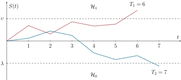
calcu-1 2 3 4 5 6 7 λ υ H1 H0 T1 = 6 T2 = 7 t S(t)

Figure 3.1:Two exemplary random walks of a test statistic in anSPRTwith corresponding runlengths.

lated according to S(y) = log(Z(y)) = K ∑ i=1 log ( p1(yi) p0(yi) ) . (3.5)

The decision rule(3.3)becomes

δ∗(y) =          0, S(y)<log(τ), 0or1, S(y) = log(τ), 1, S(y)>log(τ).

3 . 2

S e q u e n t i a l H y p o t h e s i s Te s t i n g

In sequential hypothesis testing the goal is to make a reliable decision betweenH0 andH1

based on as few measurements as possible. The most widely used hypothesis test of this kind is the Sequential Probability Ratio Test (SPRT) as introduced by Wald [Wald, 1947]. The idea is to update the test statistic(3.5)sequentially over time as new samples are taken instead of calculating it from a fixed number of samples. The decision thresholdτis then replaced by an upper thresholdυand a lower thresholdλ. These thresholds span a corridor in which the test statistic performs a random walk as shown inFigure 3.1. The decision and stopping rule

3 . 2 S e q u e n t i a l H y p o t h e s i s Te s t i n g of theSPRTreads as δ(t) =          0, S(t)≤λ, continue sampling, S(t)∈(λ, υ), 1, S(t)≥υ, (3.6) where S(t) = t ∑ i=1 log ( p1(yi) p0(yi) ) =S(t−1) + log ( p1(yt) p0(yt) ) . (3.7)

Wald showed that performing the test in this way can reduce the required number of sam-ples by up to50 %on average while retaining the same error probabilities. He furthermore provided simple bounds for the decision thresholds, namely

λ≤ 1−β

α and υ ≥

β 1−α,

which solely depend on the prespecified bounds on the probabilities of false alarm and misde-tectionαandβ, respectively.

Since in a sequential hypothesis test the number of samples is not fixed, the average run-length (ARL) is—together withP_FAandPMD—an important metric for evaluating the per-formance of a sequential detector. The runlengthT of theSPRTis defined as the first time instant where eitherH0orH1is accepted, i.e.,

T =inf{t|S(t)∈/(λ, υ)}.

Wald showed that—when neglecting the possible overshoot of the test statistic upon crossing a threshold—theexpectedrunlength of the test can be approximated by

E0[T]≈ 1 D(p1|p0) (αlog(υ) + (1−α) log(λ)), E1[T]≈ 1 D(p1|p0) ((1−β) log(υ) +βlog(λ)),

where Em[·]denotes the expectation underHm. Furthermore, D(p1|p0)is the

Kullback-Leibler divergence—a measure for the similarity of two distributions withPDFsp0andp1. It

is given by the expected value of theLLR, i.e.,

D(p1|p0) =E1 [ log ( p1(y) p0(y) )] = ∫ p1(x) log ( p1(x) p0(x) ) dx.

3 . 3

L e a s t Fav o r a b l e D e n s i t i e s

As discussed inSection 2.1, many practical applications suffer from an uncertainty about the distribution of the observed data. Taking this uncertainty into account transforms thesimple hypothesis tests in(3.1)and(3.2)intocompositetests betweenM disjoint sets of probability distributionsPmwith corresponding hypotheses

Hm :P ∈ Pm.

One possible way to characterize these sets is with the help of Kassam’s band model [Kassam, 1981;Fauß&Zoubir, 2016] as

Pm =

{

Pmp′m ≤pm ≤p′′m

}

, (3.8)

wherep′_mandp′′_mare nonnegative functions whose integral over the sample space is less than one and greater than one, respectively. Note that the inequalities in(3.8)are defined point-wise. This model is flexible as it allows for varying local degrees of uncertainty on different re-gions of the sample space. It can either be constructed by hand based on expert knowledge, or statistically using confidence interval estimators. In contrast to many parametric uncertainty models, Kassam’s model can be easily interpreted and visualized. Furthermore, it generalizes several popular uncertainty models such as theε-contamination model as will be seen shortly. All of these reasons attest to the usefulness of this model for a wide variety of applications.

Intuitively speaking, Kassam’s band model assumes the true densitypmto lie within a band

specified byp′_mandp′′_m, which can be interpreted as a confidence interval forpm. A suitable

decision rule in this case is one that is optimized for the worst case and, hence, guarantees a reliable performance for all possible cases. Tests of this kind are referred to asminimax optimal

3 . 3 L e a s t Fav o r a b l e D e n s i t i e s

orminimax robust since they minimize the maximum possible risk associated with the test (see, e.g., [Levy, 2008;Poor, 2013]). In [Fauß, 2016] aminimax robustversion of theSPRT

is introduced, which replaces theLLRin(3.7)with theLLRof theLFDsq0 andq1. Since

these probability densities represent the worst case, a test run under these conditions willat leastattain the performance specified byαandβ. Using the algorithm provided in [Fauß&

Zoubir, 2016], theLFDsfor a fixed-sample-size test are iteratively calculated according to q0 = min{p′′0,max{c0(νq0+q1), p′0}},

q1 = min{p′′1,max{c1(q0+νq1), p′1}},

(3.9)

for someν ≥ 0and somec0, c1 ∈ (0,1_ν]. Details of how to obtainLFDsthat are minimax

optimal in a sequential architecture can be found in [Fauß, 2016].

Uncertainties of theε-contamination type as defined inSection 2.1.1are included in Kas-sam’s band model by settingp′₀ = (1−ε)p◦₀,p₀′′ =p′′₁ =∞, andν = 0, so that(3.9)reduces to

q0 = max{c0q1, p′0},

q1 = max{c1q0, p′1}.

The resulting densities correspond to theLFDsof Huber’s clipped likelihood ratio test [ Hu-ber, 1965;Huber, 1981], which censors outliers and, thus, prevents them from having an un-bounded effect on the test. Due to this property, it makes sense to use the centralized, fixed-sample-sizeLFDsalso in the context of distributed sequential detection. While they are not minimax optimal in this case, they induce robustness by limiting the influence of large values at the cost of an increasedARLas will be shown inChapter 4.

4

Robust Sequential Binary

Hypothesis Testing

This chapter is concerned with binary hypothesis tests that are performed in a sequential manner in a distributed network architecture and are subject to distributional un-certainties. InSection 4.1, the problem of performing shift-in-mean and shift-in-variance tests in this setup is formulated.Section 4.2introduces a general formulation of the Consensus+In-novations Sequential Probability Ratio Test (CISPRT)—a fully distributed sequential detec-tion algorithm. The corresponding decision thresholds are derived inSection 4.3.Section 4.4

andSection 4.5present two different paradigms for robustifying theCISPRTagainst outliers of theε-contamination kind. The simulations inSection 4.6verify and evaluate the perfor-mance of the proposed algorithms in a shift-in-mean and a shift-in-variance test. The findings are summarized inSection 4.7.

The contributions presented in this chapter have been published in [Leonard&Zoubir, 2017], [Hou, Leonard et al., 2017], and [Leonard&Zoubir, 2018a].

4 . 1

P ro b l e m F o r m u l at i o n

LetY(t) ∈ RN_{, t = 1,2, . . . be a sequence of random vectors with entriesY}

k(t), k =

1, . . . , N. For allk andt the random variablesYk(t)are assumed to be independent and

identically distributed according to distributionP, which admits a densityp. In distributed sequential detection, each agentk sequentially performs a binary statistical hypothesis test to decide between the null hypothesisH0 and the alternativeH1according to(3.1). To this

end, it takes a measurementyk(t)at time instanttfrom which a test statistic is computed.

Considering a Gaussian environment, the hypotheses read as

H0 :Yk(t)∼ N(µ0, σ02),

H1 :Yk(t)∼ N(µ1, σ12),

(4.1)

whereµi, i ∈ {0,1}is the known mean andσi2the variance of a zero-mean Gaussian noise

process. While the results of this chapter can be applied to any binary hypothesis test of this type, the focus is on the following two test scenarios:

• Scenario 1: Shift-in-Mean Test

The mean of the distribution under the true hypothesis is tested for, assuming equal varianceσ2_{under bothH}

0andH1. The hypotheses become

H0 :Yk(t)∼ N(µ0, σ2),

H1 :Yk(t)∼ N(µ1, σ2).

• Scenario 2: Shift-in-Variance Test

The test is for the variance of the distribution under the true hypothesis assuming two zero-mean Gaussian distributions. An example for this is a test for the presence or ab-sence of a zero-mean signal with known varianceσ2

xin zero-mean noise with powerσn2,

i.e.,

H0 :Yk(t)∼ N(0, σ2n), H1 :Yk(t)∼ N(0, σ2x+σ

2

4 . 2 Th e C o n s e n s u s + I n n o va t i o n s S e q u e n t i a l P r o b a b i l i t y R a t i o Te s t

4 . 2

Th e C o n s e n s u s + I n n o vat i o n s S e q u e n t i a l P ro b a

-b i l i t y R at i o Te s t

In [Sahu& Kar, 2014; Sahu& Kar, 2016] the Consensus+Innovations Sequential Proba-bility Ratio Test (CISPRT) is proposed as a distributed sequential detector based on the consensus+innovationsapproach [Kar&Moura, 2013]. In analogy to the centralizedSPRT

introduced by Wald [Wald, 1947], each agent k in theCISPRTcompares its test statistic Sk(t)at time instanttwith an upper and a lower threshold to either decide for one of the

two hypotheses if the respective threshold is crossed, or to continue the test. Sk(t)is

recur-sively calculated as

Sk(t) =

∑

l∈Nk

wkl(Sl(t−1) +ηl(t)), (4.2)

withwkldenoting appropriate combination weights that sum to one. Furthermore,ηl(t)is

theLLRof nodelat time instantt, which is calculated as ηl(t) = log ( p1(yl(t)) p0(yl(t)) ) = σ 2 1(yl(t)−µ0)2−σ20(yl(t)−µ1)2 2σ2 0σ12 + log ( σ0 σ1 ) (4.3)

assuming the general formulation from(4.1). By collecting the combination weights into an N ×N combination matrix,(4.2)can be rewritten as

Sk(t) = t

∑

j=1

e⊤_kWt+1−lη(j), (4.4)

withekdenoting thekth column of identity matrixI of sizeN. TheLLRs of all agents at

time instantj are collected in the vectorη(j) = [η1(j), . . . , ηN(j)]⊤. In the sequel, the

choice of the weighting matrixW is discussed.

4 . 2 . 1 C h o o s i n g We i g h t i n g M at r i x W

In [Sahu&Kar, 2016], the authors assume a weighting matrix that is non-negative, symmetric, irreducible, and stochastic by design. However, the design process relies on a method origi-nally introduced in [Xiao&Boyd, 2004], which can—and most of the time will—produce a

matrix with negative weights on the diagonal as explicitly stated by the authors. In the context of distributed detection, such a matrix is not practical since it will cause each nodekto give its own information a negative weight. This operation has no meaning in distributed sensor networks.

Instead of requiring the weighting matrix to be doubly-stochastic, this work considers a right-stochastic matrix—i.e., its rows sum up to one. Matrices of this kind are common and well-studied, e.g., in the context of diffusion adaptation [Sayed, 2013]. An example for a right-stochastic matrix is one that puts equal weight on the information of the closed neighborhood of a node, i.e., the entries ofW are given by

wkl =    1 |Nk|, l ∈ Nk, 0, otherwise. Note that a right-stochastic matrix does not fulfill the requirement

Wt → 1

N11

⊤_,

where 1is the one-vector of lengthN. This requirement guarantees the convergence to a networkwide consensus over time. This work, however, focuses on reaching a networkwide decisionmeaning that the individual test statistics do not have to converge to the exact same value. Averaging over the individual stopping times at each node results in a networkwide

ARLof the distributed sequential detector, which is one of the performance metrics used in

Section 4.6.

4 . 3

D e c i s i o n Th r e s h o l d s f o r t h e

CI

S P R T

The decision thresholds derived in [Sahu&Kar, 2016] suffer from two disadvantages. First, they only hold for the specific case of symmetric Gaussian shift-in-mean hypothesis tests. In [Leonard&Zoubir, 2017] and [Hou, Leonard et al., 2017], these thresholds were generalized for use in arbitrary binary hypothesis tests. Second, the derivation of the thresholds relies on the symmetry ofW, an assumption that is usually not valid in distributed sensor networks. In the sequel, the generalized thresholds from [Leonard&Zoubir, 2017] and [Hou, Leonard

4 . 3 D e c i s i o n Th r e s h o l d s f o r t h e CIS P R T

et al., 2017] are improved by requiring only the right-stochasticity ofW in the derivation. First, however, expressions for the mean and the variance of the test statistic underH0and

H1are derived, which are needed in the subsequent steps.

4 . 3 . 1 M e a n a n d Va r i a n c e o f t h e Te s t S tat i s t i c

The expected value of the test statistic(4.2)under hypothesisHi, i∈ {0,1}is given by Ei[Sk(t)] = t ∑ j=1 e⊤_kWt+1−jEi[η(j)], =µη,i t ∑ j=1 e⊤_kWt+1−j1, =µη,it, (4.5)

whereEi[·]denotes taking the expectation under hypothesisHiandµη,i = Ei[η(j)]is the

expected value of theLLRunderHi.

The variance of the test statistic(4.2)under hypothesisHican be calculated as

Vari[Sk(t)] =Ei [ (Sk(t)−µη,it)2 ] , =Ei[Sk(t)2 ] −2µη,itEi [ Sk(t)2 ] +µ2_η,it2, =Ei[Sk(t)2 ] −µ2_η,it2, =Ei   ( _t ∑ j=1 e⊤_kWt+1−jη(j) )2 ₋µ2_η,it2, = t ∑ j=1 t ∑ l=1 e⊤_kWt+1−jEi[η(j)η(l)](Wt+1−l)⊤ek−µ2η,it2. (4.6)

Since the expected valueEi[η(j)η(l)]can be written as

Ei[η(j)η(l)] =    µ2_η,i11⊤ , j ̸=l, σ2 η,iI +µ2η,i11⊤ , j =l,

line of(4.6)leads to Vari[Sk(t)] =ση,i2 t ∑ j=1 e⊤_kWj(Wj)⊤ek+µ2η,i t ∑ j=1 t ∑ l=1 Wj11⊤(Wl)⊤ek−µ2η,it 2 , =σ_η,i2 t ∑ j=1 e⊤_kWj(Wj)⊤ek+µ2η,it 2_−µ2 η,it 2_, =σ_η,i2 t ∑ j=1 e⊤_kWj(Wj)⊤ek, =σ_η,i2 t ∑ j=1 e⊤_kWj−mWm(W⊤)m(W⊤)j−mek, (4.7)

with1≤m≤j. By upper-boundingWm(W⊤)mwith a scaled all-ones matrix according to

Wm(W⊤)m ≤ξ11⊤,

where the inequality holds elementwise,(4.7)becomes

Vari[Sk(t)]≤σ2η,i t

∑

j=1

e⊤_kWj−mξ11⊤(W⊤)j−mek.

Using the properties

W11⊤=11⊤,

11⊤W⊤=11⊤,

W11⊤W⊤=11⊤,

an upper bound on the variance of the test statistic can be found as

Vari[Sk(t)]≤ση,i2 t

∑

j=1

4 . 3 D e c i s i o n Th r e s h o l d s f o r t h e CIS P R T

A suitable choice forξis the maximum value of the matrixWm(W⊤)m, i.e.,

ξ=Wm(W⊤)m

max, (4.9)

where∥·∥maxis the maximum norm of a matrix. Another choice forξis the largest eigenvalue ofWm(W⊤)mdivided by the number of nodesN, i.e.,

ξ= 1

Nλmax

(

Wm(W⊤)m). (4.10)

The accuracy of this approximation can be tuned by the choice ofm and thus traded off against computational load. In most distributed sensor networks, computational power is a scarce resource, which is why it makes sense to choosem = 1. However, if more compu-tational power is available, a higher accuracy can be achieved by choosing a larger value for m.

The resulting expressions for the mean and the variance ofSk(t)depend on the mean and

the variance of theLLR. For general binary hypothesis tests according to(4.1), these quantities are given by µη,0 =− µ2 0+µ21−2µ0µ1+σ02−σ21 2σ2 1 + log ( σ0 σ1 ) , µη,1 = µ2₀+µ2₁−2µ0µ1+σ12−σ20 2σ2 0 + log ( σ0 σ1 ) , (4.11) and σ_η,2₀ = 1 2 ( 1 + σ 4 0 σ4 1 ) + (µ0 −µ1) 2 σ20 σ4 1 − σ02 σ2 1 , σ_η,2₁ = 1 2 ( 1 + σ 4 1 σ4 0 ) + (µ0 −µ1) 2 σ21 σ4 0 − σ12 σ2 0 . (4.12)

4 . 3 . 2 A l m o s t S u r e ly F i n i t e S to p p i n g Ti m e

Before the thresholds are derived, the test is shown to terminate almost surely under both hypotheses at finite stopping time or runlengthT with

T = inf{t|Sk(t)∈/ (λ, υ)},

whereλ andυ denote the lower and upper decision threshold, respectively. Following the line of argument in [Sahu&Kar, 2016], the probability of stopping after time instanttcan be upper-bounded underH0by P0(T > t)≤ Q ( λ−µη,0t ση,0 √ ξt ) so that lim t→∞P0(T > t) = 0, P0(T < ∞) = 1.

Here the functionQ(x) = √1

2π

∫_∞

x e−

u2

2 dudenotes the right tail-probability of the standard

normal distribution. The proof under the alternative hypothesis is analogous.

4 . 3 . 3 D e r i vat i o n o f t h e D e c i s i o n Th r e s h o l d s

When the sequential test at nodekstops at timet, a decision is made according to

δ(Sk(t)) =    0, Sk(t)≤λ, 1, Sk(t)≥ν.

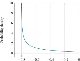
4 . 3 D e c i s i o n Th r e s h o l d s f o r t h e CIS P R T −0.8 −0.6 −0.4 −0.2 0 0 2 4 6 8 10 Probability density

Figure 4.1:Probability density function (PDF) of the log-likelihood ratio (LLR) in a sequential binary shift-in-variance test.

SinceT is finite with probability one,Sk(T)is well-defined and the probability of false alarm

at each node can be written as

PFA =P0(Sk(T)≥υ), ≤ ∞ ∑ t=1 P0(Sk(t)≥υ), ≈∑∞ t=1 Q ( υ−µη,0t ση,0 √ ξt ) . (4.13)

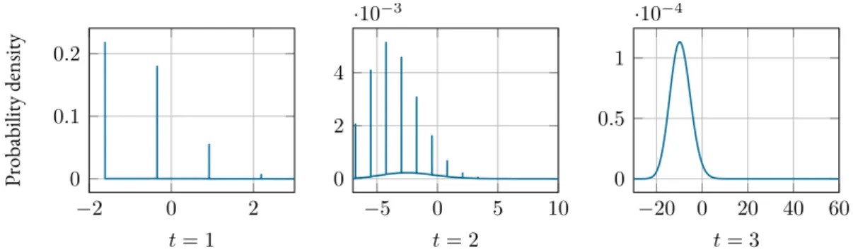
Inequality(4.13)holds true as long as the test statistic follows a Gaussian distribution. This is always the case in a shift-in-mean setup since theLLRis also Gaussian distributed. For shift-in-variance tests, theLLRfollows a chi-squared distribution with one degree of freedom as shown inFigure 4.1. Hence, it follows from the central limit theorem that(4.13)is approx-imately true after just a few time steps as depicted inFigure 4.2. Further details on this are provided inSection 4.5.2.

Using the propertyQ(x) ≤ 1₂e−x

2

−2 0 2 4 0 1 2 ·10−3 t= 1 Probability density −15 −10 −5 0 5 0 0.5 1 · 10−3 t= 2 −60 −40 −20 0 0 2 4 ·10−4 t= 3

Figure 4.2:Shift-in-variance test: evolution over time of thePDFof the test statisticSk(t)of an agent with three neighbors.

&Kar, 2016], the probability of false alarm is found to be upper-bounded by

P_FA≤ 2e υµη,0 4σ2 η,0ξ 1−e− µ2 η,0 2σ2_η,0ξ .

RequiringPFA≤αand solving forυyields the upper threshold

υ ≥ 4σ 2 η,0ξ µη,0 [ log (_α 2 ) + log ( 1−e− µ2_η,0 2σ2 η,0ξ )] . (4.14)

Repeating the same procedure for the probability of misdetection and requiringP_MD ≤ β yields the lower threshold

λ≤ 4σ 2 η,1ξ µη,1 [ log ( β 2 ) + log ( 1−e− µ2_η,1 2σ2 η,1ξ )] . (4.15)

The complete derivation of these expressions is deferred toAppendix A.2.

As mentioned in Remark 7.1 of [Sahu&Kar, 2016], the resulting thresholds pose only suf-ficient conditions on the probability of false alarm and misdetection. While tighter thresholds

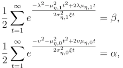
4 . 4 A R o b u s t V e r s i o n o f t h e CIS P R T B a s e d o n L e a s t Fav o r a b l e D e n s i t i e s

can be obtained by numerically solving 1 2 ∞ ∑ t=1 e −λ2−µ2_η,1t2+2_λµη,1t 2σ2 η,1ξt =β, 1 2 ∞ ∑ t=1 e −υ2−µ2_η,0t2+2_υµη,0t 2σ2 η,0ξt =α, (4.16)

the expressions in(4.14)and(4.15)are easily tractable.

4 . 4

A R o b u s t Ve rs i o n o f t h e

CI

S P R T B a s e d o n L e a s t

Fav o r a b l e D e n s i t i e s

In this section, the concept ofLFDsis used to modify theCISPRTsuch that it can deal with composite hypotheses arising from distributional uncertainties.

4 . 4 . 1 Th e R o b u s t Te s t S tat i c a n d I ts D e n s i t y

In order to design a robust version of theCISPRT, theLLRηk(t)of agentkat time instant

tin(4.2)is replaced by the corresponding clippedLLR

ηclipped_k (t) = log ( q1(yk(t)) q0(yk(t)) ) , (4.17)

i.e., theLLRof the correspondingLFDs. This yields the robust test statistic ˇ Sk(t) = ∑ l∈Nk wkl ( ˇ Sl(t−1) +η_lclipped(t) ) . (4.18)

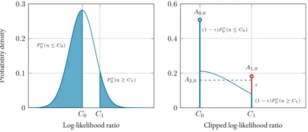
Figure 4.3compares thePDFs of theLLRand the clippedLLRside by side. By replacing the nominal densities with theLFDs, thePDFis clipped atC0 =−log (c0)andC1 = log (c1).

That way, outliers are censored, which prevents them from having an unbounded influence on the test. The excess probability that accumulates at the clipping points can be calculated

C0 C1 0 0.1 0.2 0.3 P₀◦(η≤C0) P₀◦(η≥C1) Log-likelihood ratio Probability density C0 C1 0 0.2 0.4 0.6 (1−ε)P₀◦(η≤C0) (1−ε)P₀◦(η≥C1) ε A0,0 A1,0 A2,0

Clipped log-likelihood ratio

Figure 4.3: PDFof theLLR(left) and the clippedLLR(right) underH0. ThePDFof theLLRis clipped at

C0andC1and the excess probability accumulates at the clipping points. Whenε-contamination is considered,

the probability mass is weighted by(1−ε)and the probability of drawing an outlier is added toC1. The region

between the clipping points can be approximated by a weighted uniform distribution. UnderH1, thePDFs are

mirrored at the origin.

as A0,i =Qi(ηk(t)≤C0), = (1−ε)P_i◦(ηk(t)≤C0) +iε, ≈(1−ε)Q ( −C0−µp◦_i σ2 p◦_i ) +iε, and A1,i =Qi(ηk(t)≥C1), = (1−ε)P_i◦(ηk(t)≥C1) + (1−i)ε, ≈(1−ε)Q ( C1−µp◦_i σ2 p◦_i ) + (1−i)ε,

whereµp◦_i andσ2p◦_i denote the mean and the variance of the nominal distribution underHi, i∈ {0,1}. When consideringε-contamination as defined inSection 2.1.1, the probability mass has to be scaled by(1−ε)and the probability of drawing an outlier—denoted byε—has to