Singapore Management University
Institutional Knowledge at Singapore Management University
Research Collection School Of Information Systems
School of Information Systems
6-2014
Graph-based Semi-supervised Learning: Realizing
Pointwise Smoothness Probabilistically
Yuan FANG
University of Illinois at Urbana-Champaign
Kevin Chen-Chuan CHANG
University of Illinois at Urbana-ChampaignHady Wirawan LAUW
Singapore Management University, [email protected]
Follow this and additional works at:
http://ink.library.smu.edu.sg/sis_research
Part of the
Databases and Information Systems Commons
, and the
Numerical Analysis and
Scientific Computing Commons
This Conference Proceedings Article is brought to you for free and open access by the School of Information Systems at Institutional Knowledge at Singapore Management University. It has been accepted for inclusion in Research Collection School Of Information Systems by an authorized administrator of Institutional Knowledge at Singapore Management University. For more information, please [email protected].
Citation
FANG, Yuan; CHANG, Kevin Chen-Chuan; and LAUW, Hady Wirawan. Graph-based Semi-supervised Learning: Realizing Pointwise Smoothness Probabilistically. (2014).Proceedings of the 31st International Conference on Machine Learning, Beijing, China, 21-26 June 2014. , 1. Research Collection School Of Information Systems.
Realizing Pointwise Smoothness Probabilistically
Yuan Fang†‡ [email protected]
Kevin Chen-Chuan Chang†‡ [email protected]
Hady W. Lauw? [email protected]
†University of Illinois at Urbana-Champaign, USA ‡Advanced Digital Sciences Center, Singapore
?Singapore Management University, Singapore
Abstract
As the central notion in semi-supervised learn-ing, smoothness is often realized on a graph rep-resentation of the data. In this paper, we study two complementary dimensions of smoothness: its pointwise nature and probabilistic modeling. While no existing graph-based work exploits them in conjunction, we encompass both in a novel framework of Probabilistic Graph-based Pointwise Smoothness (PGP), building upon two foundational models of data closeness and label coupling. This new form of smoothness axiom-atizes a set of probability constraints, which ul-timately enables class prediction. Theoretically, we provide an error and robustness analysis of PGP. Empirically, we conduct extensive experi-ments to show the advantages of PGP.
1. Introduction
As labeled data is often scarce, semi-supervised learning (SSL) can be beneficial by exploiting unlabeled data. Con-sider a random tuple(X, Y), where a data pointX∈ X =
{x1, . . . , x|X |}has a labelY ∈ Y. We observe labeled data
Lcomprising i.i.d. samples of(X, Y), and unlabeled data
U comprising i.i.d. samples ofX. Typically |U | |L|. Potentially, we may only observe a partialX viaLandU. The task is to predict the label for everyxi∈ U.
Towards effective SSL, graph-based smoothness has at-tracted much research interest. In particular, the smooth-nessstatement is central to SSL (Zhu,2005;Chapelle et al.,
2006): if two points xi, xj are close, their respective
la-belsyi, yj are likely to be the same. The literature further
Proceedings of the 31st International Conference on Machine Learning, Beijing, China, 2014. JMLR: W&CP volume 32. Copy-right 2014 by the author(s).
suggests that it is more effective to consider smoothness on the low-dimensional manifold, where the high-dimensional data roughly live. As widely recognized, graphs are often used as a proxy for the manifold (Blum & Chawla,2001;
Zhu et al.,2003; Zhou et al., 2003; Belkin et al., 2006;
Johnson & Zhang, 2008; Subramanya & Bilmes, 2011). Specifically, each pointxi is a node on a graph, and two pointsxi, xjmay be connected by an edge weightedWij. The weight matrixWaims to capture the pairwise geodesic distance on the manifold. In other words, the graph reveals the structures on the manifold.
Unfortunately, although graph-based methods universally hinge on smoothness, their realizations fall short. As the thesis of this paper, we advocate that smoothness shall be pointwise in nature and probabilistic in modeling.
Nature: Pointwise smoothness. Smoothness shall inher-ently occur “everywhere,” to relate the behavior of each point to that of its close points. We call this the point-wisenature of smoothness. As recently identified ( Rigol-let,2007), precisely expressing the pointwise nature boils down to two aspects:
• How do we decide if a data point is close to another? The smoothness statement lacks a concrete definition of closeness. Thus, we need adata closeness modelto de-fine this. (P1)
• How is the behavior of two close points related? The smoothness statement requires that “their labels are likely to be the same”, which is rather vague. Thus, we need alabel coupling modelto explicitly relate their la-bel behavior. (P2)
Surprisingly, to date, no existing graph-based method re-alizes pointwise smoothness. While it has been studied in non-graph based settings (Rigollet, 2007; Lafferty & Wasserman, 2007; Singh et al., 2008), previous graph-based methods treat smoothness in an aggregate, rather
Graph-based Semi-supervised Learning: Realizing Pointwise Smoothness Probabilistically than pointwise, manner. Specifically, they optimize an
energy function in a random field (Zhu et al., 2003;Zhu & Ghahramani, 2002; Getz et al., 2005) or a cost func-tion (Zhou et al.,2003;Belkin et al.,2006;Subramanya & Bilmes,2011) over the graph. An energy or cost function
aggregates all pairwise differences between neighboring points across the entire graph. By minimizing the aggre-gated difference, some “average” smoothness is achieved. However, such aggregation is not designed for and thus does not necessarily enforce smoothness at every point—it is unclear how an aggregate function can precisely express the pointwise nature of smoothness, in terms of the two aspects (P1 & P2). After all, there exist different cost func-tions varying greatly in actual forms (e.g., squared error, soft margin loss, or probability divergence), with limited justification to favor one over another.
Modeling: Probabilistic smoothness. Pointwise smooth-ness shall be modeledprobabilisticallyin both aspects (P1 & P2), to ultimately inferp(Y|X). First, how close is suffi-ciently close is difficult to be reliably captured by determin-istic binary decisions (P1). Second, the smoothness state-ment that “their labels are likely to be the same” is mean-ingless (Rigollet,2007) unless it is exploited in probabilis-tic terms (P2). Within a probabilisprobabilis-tic framework, eventu-ally each point can be classified based onp(Y|X), given i.i.d. samples. Furthermore, probabilistic modeling con-veys some concrete benefits, such as integrating class priors
p(Y)in a more principled way, naturally supporting multi-class tasks, and facilitating client applications that require probabilities as input.
We note that existing probabilistic modeling in graph-based settings (Subramanya & Bilmes,2011;Das & Smith,2012;
He et al.,2007;Azran,2007) only supports aggregate, but not pointwise, smoothness.
Our proposal.We propose the framework of Probabilistic Graph-based Pointwise Smoothness (PGP), hinging on two foundations that address the pointwise nature of smooth-ness probabilistically on a graph.
To begin with, we need adata closeness modelto determine if a point is close to another (P1). Since the graph captures the pairwise geodesic distance on the manifold, a random walk on the graph—which moves from X toX0 in each
step—naturally “connects”XandX0as close points on the manifold. Hence, for apairof random points(X, X0)such that X is close to X0, we can describe their distribution
p(X, X0)using thesecond-orderstationary distribution of the random walk. In contrast, the distribution of asingle
pointp(X)has been traditionally represented by the first-orderstationary distribution.
Next, we also need alabel coupling modelto relate the la-bel behavior of a pointxito that of its close points (P2). We
leverage the notion ofstatistical indistinguishability( Gol-dreich,2010). In particular, whetherX isxi, orXis some point close toxi, the labelY ofX shall be produced in an indistinguishable manner. In other words, we cannot tell apart the distributions ofY in these two cases.
Together, these two foundations constitute our smoothness framework, which further entails a solution to SSL. While the given labels naturally constrain the labeled data, our smoothness framework axiomatizes a set of probability constraints on the unlabeled data. Solving these constraints eventually infers p(Y|X)for class prediction. Note that the constraints can be either discriminative overp(Y|X), or generative overp(X|Y). Although the ultimate goal is
p(Y|X), generative models that learnp(X|Y)andp(Y)
are often favorable in SSL (Chapelle et al.,2006). Thus, although our framework can accommodate both forms, we adopt the generative form here and leave the discriminative counterpart to future work1.
Finally, we present a theoretical analysis of our solution. First, to see that PGP can utilize both labeled and unlabeled data, we derive a generalization error inLandU. Second, to show that PGP is not sensitive to noisy input graphs, we assess the robustness of our solution.
Our contributions. We summarize the contributions in this paper as follows.
• We propose PGP, the first work to realize pointwise smoothness on a graph probabilistically.
• We conduct an error and robustness analysis of PGP.
• We demonstrate the advantages of PGP through exten-sive experiments.
2. Smoothness Framework
To express the pointwise nature of smoothness, we must address its two aspects. Under a probabilistic graph-based framework, we propose a data closeness model to capture how a point is close to another (Sect.2.1), as well as a label coupling model to conceptualize how the label behavior of a point is related to that of its close points (Sect.2.2). 2.1. Data Closeness Model (P1)
We first propose a probabilistic model for capturing data closeness on the graph.
Graph. For a set of pointsX ={x1, . . . , x|X |}, we
con-struct a graphGto capture the pairwise geodesic distance on the underlying manifold. Each pointxi ∈ X is a ver-tex of G, and each pair of points (xi, xj) form an edge of Gwith a weightWij. Wij is also known as the
itybetweenxi andxj, an approximate description of the geodesic distance between the two points. W is often de-fined as follows: Wij= exp −kxi−xjk2/2σ2 i6=j 0 i=j, (1)
wherek·kis a symmetric distance function, andσis a scal-ing parameter. In our notation, unquantified indices such as
i, jbelong to{1, . . . ,|X |}, unless stated otherwise. Random walk-based closeness.As argued in Sect.1, it is difficult to reliably capture how close is sufficiently close in a deterministic manner. In order to develop probabilistic closeness, we need to represent the event that two points, sayxiandxj, are close.
We capture the closeness event based on a random walk on the graph. Consider a random walk onGvisiting a se-quence of points{Vt:t= 0,1, . . .}. While traditionally a
visitatxi(Vt =xi)models a single pointxi, atraversal walking from a point xi to another xj (Vt = xi, Vt+1 = xj)naturally “connects”xiandxjto imply thatxiis close toxjon the underlying manifold.
Note that our use of random walk serves a novel purpose. It specifically models the first pointwise aspect (P1) of re-lating the pointsXthrough the closeness event, which, to-gether with the second aspect (P2) of relating the labelsY
in Sect.2.2, is necessary for pointwise smoothness. On the contrary, existing use of random walk in SSL (Szummer & Jaakkola,2001;Azran,2007;Wu et al.,2012) models the “propagation” of labelY amongX altogether, without treating the two aspects explicitly.
Formally, let(X =xi, X0 =xj)denote the event thatxi is close toxj, which follows the distribution of observing a random walk traversal fromxi toxj in the long run as
t→ ∞. Hence,(X, X0)is a pair of limiting random
vari-ables in the sense that a traversal (Vt, Vt+1)converges in
distributionto(X, X0)jointly:
(Vt, Vt+1)
d
−→(X, X0). (2)
In other words, (X, X0) describes the closeness between two points with the jointsecond-orderlimit, whileX de-scribes a single point with the marginalfirst-order limit. Their convergence will be shown later.
Probability space of closeness.We describe the probabil-ity space of the random walk-based closeness model.
Sample space.An outcome thatxiis close toxjis a pair of points(xi, xj), which corresponds to a random walk traver-sal fromxi toxj. Hence, the sample space isΩ = X2. An outcome can be denoted by a pair of random variables
(X, X0)∈Ω, as defined in Eq.2.
Events. As discussed, each outcome(xi, xj)is an event thatxi is close toxj,i.e.,{(X, X0)∈ Ω :X =xi, X0 =
xj}or denoted(X =xi, X0 =xj). In order to relate the behavior of two close points, we are also interested in the events thatXisxiorXis close toxi.
First, {(X, X0) ∈ Ω : X = xi}, or denotedX = xi, is the event ofobservingX as a pointxi. It corresponds to a traversal fromxito some point.
Second,{(X, X0)∈Ω :X0 =xi}, or denoted(X, X0=
xi), is the event ofobservingX as some point close toxi (i.e., X is implicitly constrained byX0 = xi). It
corre-sponds to a traversal from some point toxi.
Without loss of generality, here we treatX as the random variable of interest, and our ultimate goal is to estimate
p(Y|X). However, we could also treatX0 as the variable of interest, and findp(Y0|X0)in a symmetric manner given thatW is symmetric.
Probability measure. Finally, we evaluate the probability of the events. The random walk can be formally repre-sented by a transition matrixQsuch that
Qij =Wij/Zi, where Zi,PjWij. (3) As (Vt, Vt+1) converges in distribution to (X, X0), the
closeness event (X = xi, X0 = xj) obeys the
second-orderstationary distribution of the random walk:
p(X=xi, X0=xj) = limt→∞p(Vt=xi, Vt+1=xj).(4)
As established in Proposition1, a unique second-order sta-tionary distribution exists. As a further consequence, the probability of the events can also be computed2.
PROPOSITION1 (PROBABILITY OF EVENTS): (a) The limit ofp(Vt, Vt+1)ast→ ∞exists uniquely.
(b) Given that(Vt, Vt+1)
d
−→(X, X0),
∀ij, p(X =xi, X0 =xj)∝Wij, (5)
∀i, p(X =xi) =p(X, X0=xi)∝Zi. (6)
Intuitively, Eq.5means that the stronger affinity Wij be-tweenxi andxj, the more likely they are close. Second, Eq. 6 implies that observing xi is as likely as observing a point close toxi, which is not surprising given that two close points lie near each other on the manifold.
2.2. Label Coupling Model (P2)
Next, we propose a label coupling model to relate the la-bel behavior of two close points. In our realization, the labelY of X distributes similarly whetherX isxi itself,
Graph-based Semi-supervised Learning: Realizing Pointwise Smoothness Probabilistically orXis some point close toxi. That is,p(Y|X=xi)and
p(Y|X, X0=xi)shall be alike.
Indistinguishability. We leverage the concept of statis-tical indistinguishability (Goldreich,2010): two distribu-tions are statistically indistinguishable if they cannot be told apart to some extent.
DEFINITION1 (INDISTINGUISHABILITY): Two distribu-tionsD1andD2are-statistically indistinguishableif and only if 12kD1−D2k1≤.
In our context,p(Y|X =xi)andp(Y|X, X0=xi)shall be statistically indistinguishable. In other words, the label
Y ofXis produced in an indistinguishable manner regard-less ofX beingxior a point close toxi.
Label Coupling.To achieve indistinguishability,xi’s label shall distribute similarly to that of a point close toxi. At the same time, some “distrust” of the close points shall be allowed, as small variances in their labels are still expected. These factors can be accounted for by a simple mixture:
p(Y|X=xi) = (1−α)p(Y|X, X0=xi) +αD, (7)
whereα∈ (0,1)is a parameter, andDis the distribution to fall back on when the close points are not trusted. In the distrust case, we assignxi to an “unknown” classφ /∈ Y,
i.e., D(y) = 0,∀y ∈ Y andD(φ) = 1. Our label cou-pling model represented by this mixture formally satisfies statistical indistinguishability.
PROPOSITION2 (LABEL COUPLING): Given Eq. 7, the label distribution ofxi,p(Y|X =xi), isα-statistically
in-distinguishable from the label distribution of some point close toxi,p(Y|X, X0=xi).
Note that Eq.7couples the label distributions in a discrim-inative form of p(Y|X). To model the generative proba-bilityp(X|Y)as Sect.1motivated, we also derive its gen-erative counterpart.∀y∈ Y,∀xi∈ X,
p(X =xi|Y =y)
=p(Y =y|X =xi)p(X =xi)/p(Y =y)
= (1−α)p(Y=y|X, X0=xi)p(X, X0=xi)/p(Y=y)
= (1−α)p(X, X0=xi|Y =y). (8)
In particular,Dis eliminated sinceD(y) = 0,∀y∈ Y,i.e., points of class y ∈ Y cannot be generated from D. The intuition is that indistinguishability slowly “fades” along a “chain” of close points due to the1−αfactor.
Implication. Eq. 8 implies that the first-order condi-tional distributionp(X =xi|Y =y)can be related to the sum of the second-order (joint) conditional distributions
p(X =xj, X0 =xi|Y =y)overxj∈ X. The association of the first-order or point distribution, to the second-order
or edge distribution, is expected, as the pointwise nature of smoothness is to relate the behavior of a pointxito that of its close pointsxj, which we shall see next.
3. Probability Constraint-based Learning
Under the smoothness framework in Sect.2, we develop a set of generative probability constraints in terms of
p(X|Y), and show that a unique solution satisfying the constraints exists. Next, we use an iterative algorithm to find the solution and predict classes accordingly.
3.1. Generative Probability Constraints
For eachy∈ Y, we aim to learn the generative distribution
πy,(πy1, . . . , πy|X |), (9)
whereπyi ,p(X =xi|Y =y). To findπy, we develop and solve a set of constraints onπy. On the one hand, for
xi ∈ L the constraints can be modeled using the known labels. On the other hand, while there is no known label for
xi ∈ L/ , the constraints can be modeled using points close toxi, based on our smoothness framework.
Labeled points. We rewritep(X =xi|Y =y)for xi ∈
L, relating it top(Y =y|X=xi)which can be estimated from the known labels in Sect.3.3. For a giveny∈ Y,
p(X =xi|Y =y)
=p(Y =y|X =xi)p(X =xi)/p(Y =y)
∝p(Y =y|X =xi)Zi (10)
The proportionality follows fromp(X=xi)∝Zi (Propo-sition1). We can transform this result into a constraint on
πybelow, whereKis the sum ofπyifor labeled points, and
θyiis the proportion eachπyigets from the sumK accord-ing to Eq.10. Note that we writep(y|xi)as a shorthand forp(Y =y|X =xi)if there is no ambiguity.
Constraint on Labeled Data:
πyi=K·θyi, ∀i:xi∈ L. (11)
where K=P
i:xi∈Lπyi,
θyi=p(y|xi)Zi/Pk:xk∈Lp(y|xk)Zk.
Unlabeled points. We also rewritep(X=xi|Y =y)for unlabeled points xi ∈ L/ , relating it to that of its close points. Specifically, for a giveny∈ Y,
p(X=xi|Y =y) 1 = (1−α)p(X, X0=xi|Y =y) 2 = (1−α)P jp(X=xj, X0 =xi|Y =y) 3 = (1−α)P jp(X0=xi|X=xj, Y=y)p(X=xj|Y=y) 4 = (1−α)P jp(X0 =xi|X =xj)p(X =xj|Y =y) 5 = (1−α)P jWji/Zj·p(X =xj|Y =y) (12)
Step 1 is the generative form of smoothness (Eq8). In step 2, we relatexito eachxjthrough their second-order (joint) distribution, where eachxj has a different probability of being close toxi. In step 3, based on our closeness model, givenX =xj,X0 =xionly depends onW and is condi-tionally independent ofY. In Step 5,p(X0 =xi|X =xj) is simply the transition probabilityQji = Wji/Zj. This result imposes another constraint onπy.
Constraint on Unlabeled Data:
πyi= (1−α)PjWji/Zj·πyj, ∀i:xi∈ L/ . (13)
3.2. Solving the Constraints
The goal is to solveπy that satisfies the constraints on la-beled and unlala-beled data. In particular, we can show that
πyis the stationary distribution of some Markov chain with
X as its state space. Intuitively, the unlabeled constraint (Eq. 13) already tells us how state xj transitions to each
xi ∈ L/ . Thus, we only need to deduce the transition to each statexi∈ L. Proposition3establishes the exact tran-sition between the states.
PROPOSITION3 (SOLUTION): ∀y ∈ Y, ifπy satisfies the constraints in Eq.11and13, then:
(a)πy is the stationary distribution of a Markov chainC with statesX and transition matrixP, where
Pji= P k:xk∈LWjk+αPk:xk /∈LWjk Zj ·θyi i:xi ∈ L (1−α)Wji Zj i:xi ∈ L/ , (14)
(b) The stationary distribution ofCexists uniquely. In fact, Eq.14means thatπy = πyP. If we rewrite it as element-wise operations, we see that a constraint is placed on every individual point.
Class prediction. Given πy (which will be solved in Sect.3.3), we predict the labelyiforxias follows:
yi= arg maxy∈Yp(Y =y|X =xi)
= arg maxy∈Yp(X=xi|Y =y)p(Y =y). (15) Herep(X =xi|Y =y)is simplyπyi, andp(Y =y)is the class prior which can be estimated fromL.
3.3. Solution Computation and Estimation Next, we discuss howπycan be computed.
Iterative algorithm. Proposition3entails thatπy can be found iteratively, if the transition matrixPisknown:
π(yt+1)=πy(t)P, t= 0,1,2, . . . , (16)
whereπ(yt)converges uniquely ast → ∞for an arbitrary initial distributionπ(0)y .
Solution estimation.We can only find a solution estimator
ˆ
πysinceP isunknown—Pis a function ofWandθy, both of which can only be estimated, resulting in two types of er-ror. First,data sampling error:Wis defined onX, but only a partialXˆis observed throughLandU. Thus, we can only construct an estimatorWˆ using the incompleteXˆ. Second,
label sampling error: θy is defined byp(y|xi),∀xi ∈ L, butp(y|xi)is unknown. We can only estimate it from the given labels,pˆ(y|xi) =|Ly∩ Lxi|/|Lxi|whereLy is the set of all samples withyinL, andLxiis the set of all sam-ples withxiinL. Subsequently, we obtain an estimatorθˆy based onpˆ(y|xi).
Efficiency. While efficiency is not our focus, PGP can be solved efficiently using standard iterative techniques, and its complexity is comparable to most existing SSL meth-ods. In terms of time, if we use a widely acceptedkNN graph, the cost isO(k|X |s), wheresis the number of itera-tions till convergence (typicallyk~10,s~100). Although constructing an exactkNN graph can be quadratic, an ap-proximate graph is often adequate (Chen et al.,2009). In terms of space, we can store thekNN graph sparsely, thus needing onlyO(k|X |)space.
3.4. Discussion: Comparison to Existing Methods Our constraints on unlabeled points (Eq.13) may appear similar to existing works, in particular GRF (Zhu et al.,
2003) of the following formulation:
Fi=PjWij/Zi·Fj, (17)
whereFi∈[0,1]is the label function atxi.
Although they resemble in the surface form, their exact forms are still disparate. We stress that such resemblance— expressingxi’s label as some function of its neighborsxj— is quite expected, since it is a common insight of graph-based SSL to relate a point and its neighbors on the graph (Zhou et al.,2003;Subramanya & Bilmes,2011). Nonethe-less, our exact function still differs in that PGP normalizes eachxjdifferently byZj and has a damping factor1−α, whereas GRF normalizes eachxjby the sameZiand has no damping factor. Beneath the surface resemblance, there also exist some fundamental differences.
First, most existing cost function (Zhou et al.,2003;Belkin et al.,2006) or random walk (Szummer & Jaakkola,2001;
Azran,2007;Wu et al.,2012) approaches, including GRF, do not correspond to an explicit formulation of pointwise smoothness. For instance, GRF boils down to the energy function of a Gaussian field, which is the aggregated sum of pairwise losses. Such aggregation is not designed for or derived from requiring smoothness at every individual point. Thus, smoothness does not necessarily occur “ev-erywhere.” Even though GRF eventually leads to a local weighted average of neighbors (Eq.17), it is a consequence
Graph-based Semi-supervised Learning: Realizing Pointwise Smoothness Probabilistically (a) Dataset x -0.4 0 0.4 0.8 1.2 1 11 21 31 41 51 59 Decision function
Sequence of points in one structure PGP GRF MP (c) Decision function x (b1) PGP x x x x (b2) GRF x x x x (b3) MP x x x x
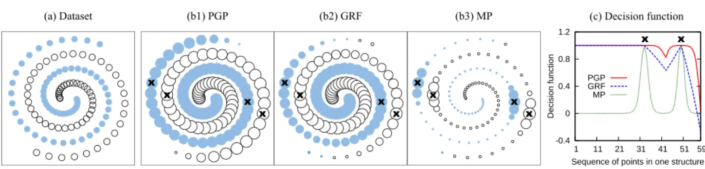
Figure 1.Toy problem: (a) Two-spiral dataset; (b1–3) Visualization of predictions and smoothness; (c) Decision function over a structure.
of minimizing an aggregate loss function, rather than origi-nating from the pointwise nature in terms of the two aspects P1 & P2. In contrast, PGP is not derived from an aggregate function, but directly builds on the data closeness model (for P1) and label coupling model (for P2).
Second, while many approaches (Zhu et al., 2003; Wu et al.,2012) have probabilistic interpretations, they do not explicitly modelp(Y|X)orp(X|Y). Taking GRF as an example,{Fi}represents the most probable configuration of a Gaussian field. Equivalently, Fi is the random walk probability that a particle starting fromxifirst hits a labeled point. Both interpretations do not explicitly correspond to
p(Y|X)orp(X|Y). In contrast, in PGP,πydirectly cor-responds top(X|Y =y).
Finally, we use a two-spiral dataset (Singh, 1998) to il-lustrate that PGP indeed results in better smoothness. As shown in Fig.1(a), the dataset consists of two spiral struc-tures as the two classes (i.e., Y = {1,2}). We compare the smoothness of PGP with the well-known GRF and the state-of-the-art MP (Subramanya & Bilmes,2011), which are both graph-based methods albeit with different energy or cost functions.
Smoothness essentially implies that the decision function
of a classifier changes slowly on a coherent structure (Zhou et al.,2003). A previously proposed decision function is
h(xi) , (H1i −H2i)/(H1i +H2i), where Hyi is xi’s “score” for class y, as assigned by a method. Then, the decision rule is sign(h(xi)), which is equivalent to the de-cision rule of every method compared here.
In Fig.1(b1–3), we visualize the predictions made by the three methods, respectively. All methods use the same four points marked by ××× as labeled, whereas the rest are un-labeled. Their respective optimal parameters are adopted. The colorof a point xi represents the predicted class yi, and thesizeof a pointxirepresents the magnitude of the decision function atxi,|h(xi)|. Thus, a smoother decision function shall result in a sequence of points in more uni-form sizes over each structure. Clearly, among the three methods, PGP generates points of the most uniform sizes,
and is smooth nearly everywhere. Alternatively, we plot the decision function over the sequence of points in one of the structures in Fig.1(c), which shows that PGP has a smoother decision function.
With better smoothness, PGP achieves a perfect result against the ideal classification in Fig.1(a) (where the size of each point has no significance). In contrast, GRF and MP misclassify 4 and 2 points, respectively.
4. Theoretical Analysis
Error inπˆy.It is crucial that we can bound the error in the solution estimatorπˆy, which is estimated from the samples
LandU.
We show that the expected error, Ekπˆy−πyk1
, can be bounded by two terms, corresponding to the two types of error discussed in Sect.3.3. Formally, as our solution is the stationary distribution of a Markov chain, the proof can be established based on the perturbation theory of Markov chains (Cho & Meyer,2001;Seneta,1993).
PROPOSITION4 (ERROR): Given the two constraints (Eq.11and13), for any constant∈(0,1),
Ekπˆy−πyk1 ≤O(1−λ1)|U | +O exp −22λ2 min xi∈L,p(y|xi)>0 |Lxi| , (18)
where λ1 = minxi∈X,p(xi)>0p(xi), and λ2 =
minxi∈L,p(y|xi)>0p(y|xi)
2
are constants in(0,1].
This result presents two major implications. First, both la-beled and unlala-beled data can help, as the bound improves whenLorU grows. Second, the bound is fundamentally limited byL. Given a fixed set ofL, even as|U | → ∞, we can achieve no better than the second error term. In other words, unlabeled data can only help so much. While our analysis is tailored to PGP, the result is consistent with previous analysis (Rigollet,2007).
graph construction function (Eq.1) is perfect. If the graph were constructed differently (i.e., perturbed), can we assess the robustness of our solution? In other words, do small perturbations only cause a small change in the solution? In our perturbation model, every pairwise affinityWijcan be perturbed by some scale factors > 1. The goal is to show that the solution derived from the perturbed affinity matrixW˜ does not change much ifsis small.
PROPOSITION5 (ROBUSTNESS): Suppose a matrixW˜ is perturbed fromW, such that for some s > 1,Wij/s ≤
˜
Wij ≤Wij·s,∀ij. Let˜πybe the the solution vector based onW˜. It holds thatkπ˜y−πyk1≤O(s2−1).
Heresis thedegree of perturbationonW. The result im-plies that our solution is robust, for changes in the solution can be bounded by the degree of perturbation.
5. Experimental Evaluation
We empirically compare PGP with various SSL algorithms, and validate the claims in this paper.
Datasets. We use six public datasets shown in Fig. 2. Three of them,Digit1,TextandUSPS, come from a bench-mark (Chapelle et al.,2006). As the benchmark datasets are mostly balanced, we also use three datasets from UCI repository (Frank & Asuncion,2010), namely,Yeast,
ISOLETandCancer3. Only a subset ofYeast(classes cyt,
me1,me2,me3) and ofISOLET(classesa,b,c,d) are used. The benchmark datasets are taken without further process-ing. For the UCI datasets, feature scaling is performed so that all features have zero mean and unit variance.
Name Task Points Features Classes Balanced
Digit1 synthetic digits 1500 241 2 yes
Text newsgroups 1500 11960 2 yes
ISOLET spoken letters 1200 617 4 yes
Cancer breast cancer 569 30 2 no
USPS written digits 1500 241 2 no
Yeast protein sites 721 8 4 no
Figure 2.Summary of the datasets.
Graph.We construct akNN graph (Chapelle et al.,2006), wherekis a parameter to be selected. To instantiate Eq.1, we use Euclidean distance for all datasets exceptText, and Cosine distance forText.σis set to the average distance of all neighboring pairs on the graph.
Labeling. For a given|L|, we sample 200 runs, where in each run|L|points are randomly chosen as labeled, and the rest are treated as unlabeled. The sampling ensures at least
3
It is known as “Breast Cancer Wisconsin (Diagnostic)” in the UCI repository.
one labeled point for each class.5%of the runs are reserved for model selection, and the remaining are for testing. Evaluation. We evaluate the mean performance over the testing runs on each dataset. As classification accuracy is not a truthful measure of the predictive power on imbal-anced datasets, we adoptmacro F-measure(Forman,2003) as the performance metric.
5.1. Comparison to Baseline Algorithms
We compare PGP to five state-of-the-art SSL algorithms, which have been shown (Zhu et al., 2003; Belkin et al.,
2006; Subramanya & Bilmes,2011) to significantly out-perform earlier ones such as TSVM (Joachims,1999) and SGT (Joachims,2003).
• Gaussian Random Fields (GRF) (Zhu et al.,2003): a pi-oneering method based on Gaussian fields, equivalent to optimizing the squared loss.
• LapSVM (LSVM) (Belkin et al., 2006): an effective graph-based extension of SVM.
• Graph-based Generative SSL (GGS) (He et al.,2007): a probabilistic generative approach.
• Measure Propagation (MP) (Subramanya & Bilmes,
2011): a divergence-based optimization formulation over probability distributions.
• Partially Absorbing Random Walk (PARW) (Wu et al.,
2012): a random walk method on graphs.
An existing implementation (Melacci & Belkin,2011) is used for LSVM, whereas our own implementations are used for the others. Each algorithm integrates class priors as suggested in their respective work, if any.
Model selection is performed on the reserved runs. For each algorithm, we searchk ∈ {5,10,15,20,25}to con-struct thekNN graph. GRF and GGS has no other parame-ters. For LSVM, we searchγA∈ {1e–6,1e–4, .01,1,100},
r∈ {0,1e–4, .01,1,100,1e4,1e6}. For MP, we search α ∈ {.5,1,5,20,100},u∈ {1e–8,1e–6,1e–4, .01, .1,1,10},
v ∈ {1e–8,1e–6,1e–4, .01, .1}. For PARW, we search
α ∈ {1e–8,1e–6,1e–4, .01,1,100}. For PGP, we search
α∈ {.01, .02, .05, .1, .2, .5}.
The mean macro F-measures on the testing runs are re-ported in Fig.3, leading to the following findings.
First, PGP performs thebestor not significantly different
from the best in 15 out of the 18 cases (i.e., columns), whereas GRF, LSVM, GGS, MP and PARW perform as such in only 3, 6, 4, 7, 5 cases, respectively.
Second, while PGP has relatively stable performance across all the cases, the baselines can be volatile. In partic-ular, when PGP is not the best, there is no consistent best method, which varies between LSVM, GGS and MP.
Graph-based Semi-supervised Learning: Realizing Pointwise Smoothness Probabilistically
|L|= 10 |L|= 20 |L|= 150
Digit1 Text ISOLET Cancer USPS Yeast Digit1 Text ISOLET Cancer USPS Yeast Digit1 Text ISOLET Cancer USPS Yeast
GRF .894 .451 .627 .871 .638 .510 .932 .467 .686 .913 .682 .569 .979 .744 .849 .958 .902 .718 LSVM .833 .428 .719 .886 .698 .562 .935 .472 .780 .914 .780 .614 .979 .771 .901 .956 .908 .729 GGS .855 .567 .677 .867 .666 .540 .886 .648 .771 .918 .758 .578 .965 .771 .905 .948 .906 .727 MP .901 .558 .692 .898 .713 .574 .940 .611 .735 .924 .794 .617 .979 .746 .854 .957 .913 .718 PARW .881 .587 .721 .893 .706 .575 .923 .640 .782 .920 .791 .613 .975 .729 .897 .955 .916 .715 PGP .910 .592 .734 .910 .704 .593 .939 .634 .786 .927 .796 .633 .978 .732 .902 .958 .931 .721 Figure 3.Performance comparison. In each column, thebestresult and thosenot significantly different(p > .05int-test) are bolded.
Third, PGP is especially advantageous with limited labeled data (e.g., |L| = 10), which is the very motivation of SSL. In contrast, when abundant data are labeled (e.g.,
|L|= 150), all algorithms perform better, and thus not sur-prisingly, the margin between them becomes smaller. 5.2. Integrating Class Priors
A concrete benefit of probabilistic modeling is to enable better integration of class priors, which is also probabilis-tic in nature. We demonstrate that principled integration of class priors is more effective than heuristics, and integrat-ing more accurate priors helps.
Integration of priors. We compare two different methods of integrating class priors:
• BAYES: integrating in PGP in a Bayesian way (Eq.15).
• CMN: integrating in GRF using the popular heuristic Class Mass Normalization (Zhu et al.,2003).
Note that BAYES and CMN respectively apply to a differ-ent algorithm as they are originally intended for. The priors are approximated in the same way for both methods, using the labeled points with add-one smoothing.
We study the corrective power of each method: integrat-ing priors can be seen as “corrections” to thebase model
that does not incorporate priors. Directly assessing the im-provement over the base model is unfair, since the base per-formances of PGP and GRF differ. Instead, we compute the F-score from the precision and recall of the corrections:
precision=#true corrections/#corrections made (19) recall=#true corrections/#corrections needed (20) The results are presented in Fig. 4(a) on the imbalanced datasets, which are more interesting given their non-uniform class priors. In all but one case, BAYES possesses much better corrective power than CMN.
More accurate priors. If class priors are integrated ap-propriately, using more accurate priors is expected to im-prove the performance. Suppose we know the exact priors by considering the labels of all points. We then apply the approximate and exact priors to PGP. We directly measure
the performance with or without priors, given the same base model. The results are presented in Fig.4(b), which illus-trate that, while the estimated priors are effective in most cases, the supposedly more accurate exact priors can fur-ther improve the performance.
(a) Corrective power of different integration methods |L|= 10 |L|= 20 |L|= 150
Cancer USPS Yeast Cancer USPS Yeast Cancer USPS Yeast
CMN .449 .264 .310 .255 .275 .307 .087 .250 .084 BAYES .333 .564 .388 .373 .692 .504 .475 .781 .607
(b) Using different priors on PGP
|L|= 10 |L|= 20 |L|= 150
Cancer USPS Yeast Cancer USPS Yeast Cancer USPS Yeast
None .923 .636 .568 .927 .722 .600 .950 .873 .678 Approx .910 .704 .593 .927 .796 .633 .958 .931 .721 Exact .929 .733 .622 .937 .805 .647 .960 .932 .730 Figure 4.Effect of incorporating class priors in prediction.
6. Conclusion
We proposed a novel framework of Probabilistic Graph-based Pointwise Smoothness (PGP), hinging on the foun-dational data closeness and label coupling models. We further transformed such smoothness into a set of prob-ability constraints, which can be solved uniquely to infer
p(Y|X). We also studied the theoretical properties of PGP in terms of its generalization error and robustness. Finally, we empirically demonstrated that PGP is superior to exist-ing state-of-the-art baselines.
Acknowledgement
This material is based upon work partially supported by NSF Grant IIS 1018723, the Advanced Digital Sci-ence Center and the Multimodal Information Access and Synthesis Center of University of Illinois at Urbana-Champaign, and Agency for Science, Technology and Re-search of Singapore. Any opinions, findings, and conclu-sions or recommendations expressed in this publication are those of the author(s) and do not necessarily reflect the views of the funding agencies.
References
Azran, Arik. The rendezvous algorithm: Multiclass semi-supervised learning with markov random walks. In
ICML, pp. 49–56, 2007.
Belkin, M., Niyogi, P., and Sindhwani, V. Manifold reg-ularization: A geometric framework for learning from labeled and unlabeled examples.J. of Machine Learning Research, 7:2399–2434, 2006.
Blum, A. and Chawla, S. Learning from Labeled and Un-labeled Data using Graph Mincuts. InICML, pp. 19–26, 2001.
Chapelle, O., Sch¨olkopf, B., and Zien, A. (eds.). Semi-supervised learning. MIT Press, Cambridge, MA, 2006.
Chen, Jie, Fang, Haw-ren, and Saad, Yousef. Fast approxi-matekNN graph construction for high dimensional data via recursive lanczos bisection. J. of Machine Learning Research, 10:1989–2012, 2009.
Cho, Grace E and Meyer, Carl D. Comparison of pertur-bation bounds for the stationary distribution of a Markov chain.Linear Algebra and its Applications, 335(1):137– 150, 2001.
Das, D. and Smith, N.A. Graph-based lexicon expansion with sparsity-inducing penalties. InNAACL-HLT, 2012.
Forman, George. An extensive empirical study of feature selection metrics for text classification. J. of Machine Learning Research, 3:1289–1305, 2003.
Frank, A. and Asuncion, A. UCI machine learning repos-itory. http://archive.ics.uci.edu/ml, 2010. University of California, Irvine, School of Information and Computer Sciences.
Getz, Gad, Shental, Noam, and Domany, Eytan. Semi-supervised learning–a statistical physics approach. In
ICML Workshop on Learning with Partially Classified Training Data, 2005.
Goldreich, Oded. A primer on pseudorandom generators, volume 55. American Mathematical Society, 2010. He, J., Carbonell, J., and Liu, Y. Graph-based
semi-supervised learning as a generative model. In IJCAI, 2007.
Joachims, T. Transductive inference for text classification using support vector machines. InICML, pp. 200–209, 1999.
Joachims, Thorsten. Transductive learning via spectral graph partitioning. InICML, pp. 290–297, 2003.
Johnson, Rie and Zhang, Tong. Graph-based semi-supervised learning and spectral kernel design. IEEE Transactions on Information Theory, 54(1):275–288, 2008.
Lafferty, John and Wasserman, Larry. Statistical analysis of semi-supervised regression. InNIPS, 2007.
Melacci, Stefano and Belkin, Mikhail. Laplacian Support Vector Machines Trained in the Primal. J. of Machine Learning Research, 12:1149–1184, March 2011.
Rigollet, Philippe. Generalization error bounds in semi-supervised classification under the cluster assumption.J. of Machine Learning Research, 8:1369–1392, 2007.
Seneta, E. Sensitivity of finite markov chains under pertur-bation. Statistics & probability letters, 17(2):163–168, 1993.
Singh, Aarti, Nowak, Robert, and Zhu, Xiaojin. Unlabeled data: Now it helps, now it doesn’t. InNIPS, pp. 1513– 1520, 2008.
Singh, Sameer. 2D spiral pattern recognition with possi-bilistic measures. Pattern Recognition Letters, 19(2): 141–147, 1998.
Subramanya, A. and Bilmes, J. Semi-supervised learning with measure propagation. J. of Machine Learning Re-search, 12:3311–3370, 2011.
Szummer, Martin and Jaakkola, Tommi. Partially labeled classification with Markov random walks. InNIPS, pp. 945–952, 2001.
Wu, Xiao-Ming, Li, Zhenguo, So, Anthony M, Wright, John, and Chang, Shih-Fu. Learning with partially ab-sorbing random walks. InNIPS, pp. 3086–3094, 2012.
Zhou, Dengyong, Bousquet, Olivier, Lal, Thomas Navin, Weston, Jason, and Sch¨olkopf, Bernhard. Learning with local and global consistency. In NIPS, pp. 321–328, 2003.
Zhu, Xiaojin. Semi-supervised learning literature sur-vey. Technical Report 1530, University of Wisconsin-Madison, 2005.
Zhu, Xiaojin and Ghahramani, Zoubin. Towards semi-supervised classification with markov random fields. Technical Report CMU-CALD-02-106, School of Com-puter Science, Carnegie Mellon University, 2002. Zhu, Xiaojin, Ghahramani, Zoubin, and Lafferty, John.
Semi-supervised learning using Gaussian fields and har-monic functions. InICML, pp. 912–919, 2003.