Full Length Article
Support vector machine based fault classification and location
of a long transmission line
Papia Ray
a,⇑, Debani Prasad Mishra
baDepartment of Electrical Engineering, Veer Surendra Sai University of Technology, Burla, Odisha, India b
Department of Electrical and Electronics Engineering, International Institute of Information Technology, Bhubaneswar, Odisha, India
a r t i c l e i n f o
Article history:Received 28 December 2015 Revised 19 March 2016 Accepted 4 April 2016 Available online 20 April 2016 Keywords:
Fault classification Feature selection Fault location Support vector machine Wavelet packet transform Transmission line
a b s t r a c t
This paper investigates support vector machine based fault type and distance estimation scheme in a long transmission line. The planned technique uses post fault single cycle current waveform and pre-processing of the samples is done by wavelet packet transform. Energy and entropy are obtained from the decomposed coefficients and feature matrix is prepared. Then the redundant features from the matrix are taken out by the forward feature selection method and normalized. Test and train data are developed by taking into consideration variables of a simulation situation like fault type, resistance path, inception angle, and distance. In this paper 10 different types of short circuit fault are analyzed. The test data are examined by support vector machine whose parameters are optimized by particle swarm optimization method. The anticipated method is checked on a 400 kV, 300 km long transmission line with voltage source at both the ends. Two cases were examined with the proposed method. The first one is fault very near to both the source end (front and rear) and the second one is support vector machine with and without optimized parameter. Simulation result indicates that the anticipated method for fault classification gives high accuracy (99.21%) and least fault distance estimation error (<0.21%) for all discussed cases. In order to verify the accuracy of the proposed method, a comparison is carried out with methods published by other researchers. Separate investigation is also carried out with the transmission line placing thyristor controlled series capacitor in the middle and applying the same proposed method. It is observed from the test results of the thyristor controlled series capacitor based transmission line model that fault classification gives a high accuracy of 98.36% and absolute fault location error is >0.29%.
Ó2016 Karabuk University. Publishing services by Elsevier B.V. This is an open access article under the CC BY-NC-ND license (http://creativecommons.org/licenses/by-nc-nd/4.0/).
1. Introduction
Progress of a country is measured by per capita consumption of electric energy. Protection engineers find it difficult to maintain uninterrupted electric power to the end users due to the presence of fault in a transmission line [1]. Generally the reason for the transmission line fault is hard to discover, so it is very important to build up a fault analyzer that can examine the type of the fault and estimate the fault distance quickly and accurately. Fault occur-rence takes place when conductors touch each other or the ground
[2], and are classified in a three phase system as: Single line-to-ground fault (SLG).
Line-to-line fault (LL).
Double line-to-ground fault (LLG). Triple line fault (LLL).
After the occurrence of a fault, restoration of power supply is possible only when the maintenance crew finishes the repair work. If failure of power supply is elongated then it leads to line outage, economic losses and wastage of time and energy of maintenance workers. So it is required to classify and locate the fault quickly and correctly, otherwise the whole transmission line has to be examined by the maintenance worker in order to find the exact fault position.
In the recent past, many researchers have investigated in a long transmission line following fault location and classification tech-niques[3]
Impedance measurement based technique. Traveling wave phenomenon based technique. Artificial Intelligence based technique. http://dx.doi.org/10.1016/j.jestch.2016.04.001
2215-0986/Ó2016 Karabuk University. Publishing services by Elsevier B.V.
This is an open access article under the CC BY-NC-ND license (http://creativecommons.org/licenses/by-nc-nd/4.0/). ⇑Corresponding author.
E-mail addresses: [email protected] (P. Ray), [email protected] (D.P. Mishra).
Peer review under responsibility of Karabuk University.
Contents lists available atScienceDirect
Engineering Science and Technology,
an International Journal
Impedance measurement based technique mainly depends on fundamental frequency current and voltages. This method is sim-ple and cheap, but gives erroneous results for huge value of the fault resistance [4]. Estimation of fault type and distance with impedance based technique in a transmission line is discussed in
[5–10]. In these schemes, single ended impedance measurement is used to estimate fault distance in a long transmission line. The simulation results of these schemes show that due to large fault resistance, estimation of fault type and distance error becomes more. In a transmission line for estimation of fault type and distance, the relationship between forward and backward waves travelling is the main theory behind travelling wave technique which has attracted widespread attention nowadays. These tech-niques estimate different type of fault and find the high impedance fault in the transmission line almost accurately, but the sampling rate required is quite high (above 1 MHz) which is hard to imple-ment in practical field [11,12]. Travelling wave based distance evaluation and fault classification in a long transmission line is reported in[13–16]. In order to analyze the fault, these schemes are based on correlation method to find the time difference between forward and backward wave. The methods discussed in
[13–16]gives less error for fault classification and distance evalu-ation, however, they show the same pattern for fault near and at the far end of the transmission line due to which it becomes quite difficult to identify and locate the fault.
Nowadays, researchers are giving more emphasis on artificial intelligence based fault classification and distance estimation skills such as neural network, fuzzy logic etc. because of its accuracy, self adaptiveness and robustness to parameter variations. Fault classi-fication with fuzzy logic technique in a long transmission line is reported in[17–20]. These schemes use wavelet transform (WT) of the current signal to provide unseen fault data to the fuzzy logic system for fault classification. In these schemes simple computa-tional process is used, however the fault classification error reported is quite large due to changes in simulation condition. Artificial neural network (ANN) is discussed in[21–28]for long transmission line fault classification and distance evaluation. These schemes[21–28]use wavelet transform or wavelet packet trans-form (WPT) to extract distinctive features like energy and entropy from acquiring signals of voltage and current which are further used in ANN for fault location and classification . The simulation results show good accuracy, however the training time is quite large due to which the task becomes quite complex and lethargic. In the scheme[29]fault classification and location in a high voltage power transmission line is proposed by using wavelet transform and support vector machine whereas in our proposed method,
fault classification and location in a high voltage power transmis-sion line is discussed by using wavelet packet transform and particle swarm optimization based support vector machine in combination with forward feature selection method. By using wavelet packet transform more number of features and better resolution is achieved. In scheme [29]one terminal current and voltage signal is analyzed and wavelet entropy criterion is applied to reduce the size of feature vectors whereas in our proposed method one terminal current signal is analyzed and wavelet energy and entropy is applied for pre-processing. Further in the proposed method, forward feature selection method is used to remove redundant features and to enhance the accuracy. It was observed from scheme[29]that fault classification accuracy was 99% and maximum fault location error was 0.74% whereas the pro-posed method in this paper says fault classification accuracy is 99.21% and fault location error is >0.21%.
Fault location of a transmission line using stationary wavelet transform in combination with determinant function feature (DFF), support vector machine (SVM) and support vector regres-sion (SVR) is discussed in [30]. The scheme in [30] uses single end measurement and DFF to extract features. Also filtering is used in the scheme [30] to remove noise and decaying DC offset. Simulation results of [30] show fault location error to be less, however the instrumentation associated with it is quite complex. Fault detection, classification and location for transmission system with multigenerators applying discrete orthogonal stockwell trans-form is reported in[31]. In this scheme[31], synchronized current measurements from both ends of the transmission line is taken for fault analysis purpose. Also in the scheme [31] energy is extracted as feature from the acquired signal and SVM is used as fault locator. However the algorithm is quite complex and parame-ters of SVM are not optimized which leads to errors in fault analysis. This paper mainly focuses on two hybrid methodologies for estimation of fault type and distance in a long transmission line. The proposed method uses one cycle waveform of current which is extracted from the sending terminal of the power system trans-mission line under study for fault classification and location. Thereafter current samples are pre-processed by wavelet packet transform and characteristics (also termed as features) like energy and entropy are extracted from them. The best feature subset of the whole feature matrix is then selected by forward feature selec-tion technique during training. The data for training is generated by considering a variety of simulation condition like type of fault, fault resistance, fault distance and fault inception angle. Further the feature set is scaled between [1, +1] which is then fed to the support vector machine (SVM) for training the data and to Nomenclature List of symbols V volts I current x(t) signal
x mean value of current signal
t time (s)
E energy
EN entropy
c cost parameter of support vector machine g gamma parameter of support vector machine f fitness value of particle swarm optimization y(k) discrete samples
e(w) evaluation function of forward feature selection method
w inertia weight in the case of particle swarm optimiza-tion
c1, c2 acceleration constant in case of particle swarm opti-mization
wmin, wmax initial and final values of weighting coefficients in case of particle swarm optimization method
Es voltage source at the sending end of the transmission line
Er voltage source at the receiving end of the transmission line
Rf fault resistance (in ohms) h fault inception angle (in degree)
e error
select the optimal features. The test data matrix is developed in an analogous way as training data matrix, but the operating condi-tions, taken is different in order to make the technique robust to parameter variation. Thereafter the test data set is validated in the trained SVM model for fault classification and location. Particle swarm optimization (PSO) technique is used to choose favorable parameters of SVM. For fault classification, four SVC are considered where three of them are placed in the three phases and the fourth one is connected between phase and ground to detect ground involvement. The sampling frequency taken for the whole process is 30 kHz. The simulation results show that the proposed tech-niques classifies and locates the fault in long transmission line fast and accurately as compared to approaches proposed by other researchers. Separate investigation with the same proposed method is also carried out with thyristor controlled series capaci-tor (TCSC) placed at the middle of the transmission line.
The remaining sections of the paper are set as follows. Brief overviews of the wavelet packet transform and feature extraction process is focused on Section2. In Section3, the forward feature selection method is discussed. Section 4 reports an article on SVM and selection process of the parameters of SVM by the particle swarm optimization technique. In Section 5, the two proposed methods for fault location and classification are discussed in details. Section6 gives the simulation results for the estimation of fault type and distance. In Section7, a comparison and discus-sion with other researchers work is made. Section8reports fault classification and location in a TCSC based transmission line with the same proposed method and Section9draws the conclusion.
2. Wavelet packet transform and feature extraction
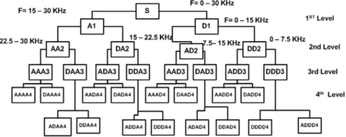
Wavelet packet transform has popularly gained attention of researchers because in some cases critical data are placed in the high frequency component of the decomposed signal which needs to be explored [22]. WPT is a generalization of discrete wavelet transform (DWT) where the discrete time signal passes from a series of filters than DWT. The DWT does not give the best result if small values of the signal are required since it is limited to wavelet bases that increase in each step with a power of two. So, in those cases another combination of bases is required which gives better result and thus WPT comes into the picture. In WPT the signal (S) goes through a series of filters (low and high pass filter) and simultaneously approximation coefficients (a) (low frequency) and detail coefficients (d) (high frequency) are formed. Thereafter the low (a) and high (d) coefficients are decomposed recursively up to levelkto make the total decomposition structure which is given inFig. 1whereas in case of DWT each step of the process is found by passing only the preceding low frequency
coefficient (a) through high and low pass filter. Also in case of WPT, after the decomposition process for each levelj2k, there are 2j numbers of node available [32]. Thus WPT gives more numbers of features, better frequency resolution, explores the information content in the high frequency component and pro-vides a global view of the decomposed signal[32]. In the present work sampling frequency considered is 30 kHz, number of sample points is 600 per signal, so up to 4th level decomposition is per-formed which is based on Shannon’s entropy criterion of optimal decomposition[33]. According to this criterion[33], at each level entropy of the signal is calculated in order to find optimal decomposition. Signal is said to obtain optimal decomposition when the entropy of parent level is higher than the total entropy of decomposed level and a single piece of information is left to reconstruct the original signal.
In order to minimize the dimension of huge data matrix, extraction of feature is used in pattern recognition where it con-verts the whole data matrix into feature matrix. In the present work two statistical features, i.e. energy and entropy are obtained from the decomposed coefficient of WPT at each sub-band. In the present work 16 decomposed WPT coefficients (32) are generated.
Energy is mathematically defined as[22,34,35]:
Eðt1;t2Þ ¼
Z t2
t1
ðjxðtÞjÞ2
dt ð1Þ
where, signal is shown byx(t), signal energy from the time range (t1,t2) by the symbolE. The value of transient energy signal is more as compared to the value of undistorted or normal signal. Signal information content is measured by entropy[34,35]. Additive infor-mation cost function[22]ofx(t) signal is defined by entropy ‘EN’ such thatE(0) = 0 and is defined as[22]:
ENðxÞ ¼X
i
ENðxiÞ ð2Þ
where, the decomposed coefficient of the signalx(t) is (xi). Entropy has large value of transient signal, whereas its value is small for normal signal. Here, a set of 32 features (2 statistical features16 WPT coefficients) is developed.
3. Forward feature selection method
Feature selection is the process which chooses features which correctly correlates the target and removes redundant ones. This method is important to implement as a large number of redundant features are used as input in several cases of supervised learning tasks which increases the computational burden and gives erroneous output which needs to be removed [36]. The feature selection method selects favorable features (those which are able
to predict the target properly) from the total matrix[36]. Feature selection is a robust greedy algorithm which avoids over fitting
[36]. Present work focuses on forward feature selection method where computation is performed in each step iteratively to choose favorable features (those showing highest scores) thus developing a subset of inputs and removing the redundant features[37]. In this paper forward feature selection method is applied. Evaluation function for the present used feature selection method is leave one out (LOO) mean square error (MSE) of the k-nearest-neighbor (KNN) estimator which provides an excellent estimate of the expected generalization error[38,39]. The weighted average of near-est neighbor is defined as KNN near-estimator, where every neighbor’s weight is proportional to its proximity[39]and the definition of eval-uation function is the negative (halved) MSE of the weighted KNN estimator[39]. The locally optimal weight vector is searched by the evaluation function which produces scores to the weight vector (w) over the features[39]. Further rank is given by the resulting weight to each feature which makes a subset of the best features.
4. Support vector machine
Statistical learning concept with an adaptive computational learning method is defined as support vector machine (SVM). This learning technique uses input vectors to map nonlinearly into a feature space whose dimension is high[40]. To make the most of the capability of the fault classifier and locator, the optimal hyper plane is determined [40]. Training algorithm of an SVM fault classifier for a given train data set which belongs to one of the two categories of the target variable [1, 1] builds a model which is shown by space mapped features where the other features are categorized by a transparent broad gap[40]. The two categories are separated by a gap which is called a hyper plane. The present work uses a radial basis function (RBF) as kernel parameter which maximizes the gap between the two categories, thereby making the hyper plane optimal[40]. Further the test data set features are mapped into that same hyper plane and predicted by the trained SVM model [40]. The merits of SVM are it does not converge into local minima, prone to overfitting, sparse and gives a global solution. Selection of proper SVM parameters is very important for good generalization performance and high accuracy in fault location and classification of transmission line [41,42].
Support vector classification (SVC) is used for classification pur-pose and support vector regression (SVR) for fault location.
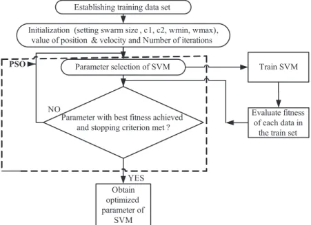
In the present work, SVM parameters are explored by integrat-ing software called LIBSVM[43]and optimal values are evaluated by (PSO) particle swarm optimization technique. The additional values taken from LIBSVM are gamma parameter (g) and soft parameter or cost parameter (c). The tradeoff between forced, rigid margin and train error is given by soft parameter or cost parameter (c)[44]and the radius and shape of the hyper plane is controlled by gamma parameter (g) [44]. Also by increasing gamma parameter, the number of support vector increases[44]. The most favorable value of SVM parameter is determined by PSO, which is as shown by flowchart in Fig. 2. The fitness value ffor the PSO is assumed as the residual mean square value (MSE) which is represented mathematically as:
f¼ ffiffiffiffiffiffiffiffiffiffiffiffiffiffiffiffiffiffiffiffiffiffiffiffiffiffiffiffiffiffiffiffiffiffiffiffiffiffiffiffiffiffi 1 N XN k¼1 yKðkÞ yðkÞ ½ 2 v u u t ð3Þ
where,y(k) is the actual discrete signal, the SVM output predictor is yK(k) and the discrete samples is denoted byN. The most favorable values of SVM parameters are selected by PSO during the training process. In the present paper, nu-svr has been considered for fault location and nu-svc for fault classification where an adaptable regularization parameter
m
(nu) is present to adjust the input data. Also, lower border on the fraction of support vectors and upper border on the fraction of margin errors is done by the SVM parameterm
(nu)[41]. Features lying near the boundary are called support vectors. The parameterm
(nu) determines the loss function (e
) by adapting the error model. Brief algorithm of nu-SVR is discussed in[45]. Nu-SVC uses a parameter nu (n) to control the number of support vectors and training errors. This parameter is sometimes symbolizes asm
2 ð0;1. This parameter nu is a lower bound on the fraction of support vectors and upper bound on the fraction of training errors. Nu (n) is a parameter of Nu-SVC whose default value is 0.5.5. Proposed technique for fault classification and location Hybrid SVM based scheme for estimation of short circuit fault type and distance in a long transmission line is discussed in this
YES NO
Establishing training data set
Initialization (setting swarm size , c1, c2, wmin, wmax), value of position & velocity and Number of iterations
Parameter selection of SVM
Parameter with best fitness achieved and stopping criterion met ?
Evaluate fitness of each data in
the train set
Obtain optimized parameter of SVM Train SVM PSO
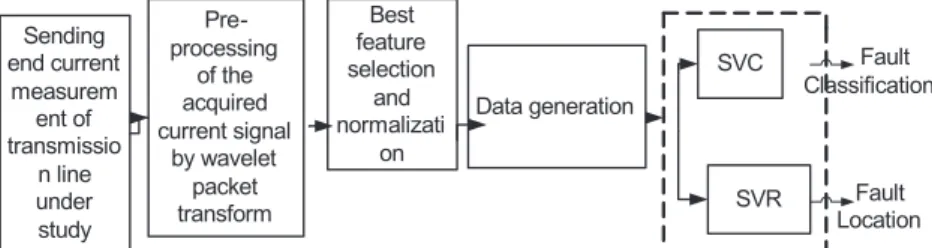
paper which is shown in Fig. 3. Post fault sending end current waveform with one cycle is used to analyze the fault type and distance in a long transmission line. The acquired samples of the sending end current signal are divided into a large range of fre-quency sub-bands using WPT. Thereafter, from the decomposed coefficient, energy and entropy are extracted. The total feature set consists of 32 features (16 WPT coefficients2 features). Fur-ther to scale feature set, normalization process is done between [1, +1] so that it can be compared appropriately. The data is then generated for training and testing purpose considering a variety of simulated conditions like the fault resistance, fault inception angle, type of short circuit fault and fault distance. Now to develop the method insensitive to parameter variations, the simulation condi-tion for generating train data matrix is made totally apart from the test data matrix. From the total feature set, some of the features don’t predict the output properly. As a result the prediction accu-racy reduces. So to improve the accuaccu-racy, redundant features are removed from the total data set by applying forward feature selec-tion technique during training. By using this feature selecselec-tion method, the total feature set to be fed to the PSO based SVM is reduced, which in turn simplifies the process and makes it fast. The optimal feature set with the test data are then fed to the trained SVM model for prediction purpose. The layout of the dis-cussed fault classification technique is presented in Fig. 4. In
Fig. 4, three SVC is placed in phasea,bandcto classify phase fault and the fourth SVC is connected between phase and ground to detect ground fault. The output of SVC placed in phasesa,band care either ‘+1’ or ‘1’ denoting faulted phase. Often double line to ground (LLG) fault is mis-classified as line-to-line fault (LL) by SVC[46]. So to overcome the difficulty a separate SVC is placed between phase and ground where a zero sequence current based indicator proposed in[47]is applied as an index value as shown in(4)and a threshold value is set by trial and error. In this paper, threshold value taken is 0.05. Ground detection is indicated when
the index value becomes more than the threshold value and it is carried out in parallel with phase identification. The detailed struc-ture of fault classifier is given inFig. 4.
Current index¼ jIaþIbþIcj
meanðjIaj;jIbj;jIcjÞ ð
4Þ
where,Ia,Ib,Icare the instantaneous values of current signal. In case of faults classification, the performance criterion considered is classification accuracy[47]which is defined as
Classification accuracy¼Accurate fault classification
Number of samples tested 100 ð5Þ
The description of the discussed fault distance estimation scheme is presented by the flowchart inFig. 5. For estimating the fault distance, the performance criterion taken is absolute error and the mean error. Mean error is defined in(6)and absolute error
[46]is defined in(7).
Mean error¼je1þe2þe3þ enj
n 100 ð6Þ
where,e1,e2,enare the ‘n’ number of absolute errors.
Absolute error¼jPr edicted fault locationExact fault locationj Total length of the line
100
ð7Þ
The transmission system under study in the present work is a 300 km long transmission line with 400 kV source at both ends and 50 Hz system frequency which is as shown inFig. 6. InFig. 6
the sending or relaying end voltage is denoted byEsand the receiv-ing end voltage is denoted byEr. Two voltage sources placed at the front and rear ends of the transmission line are represented as ideal one with its internal impedance.Appendix Agives the detail
Sending end current measurem ent of transmissio n line under study Pre-processing of the acquired current signal by wavelet packet transform Best feature selection and normalizati on SVC SVR Fault Classification Fault Location Data generation
Fig. 3.Block diagram of SVM based fault classification and location in a transmission line.
current measurement from sending end of the transmission line under study Signal decomposition and feature extraction by WPT Best feature selection by forward feature selection method SVC-g as ground detector a y b y c y SVC-a SVC-b SVC-c Support vector machine
(SVC-p) in phase a, b, c
g y
description of parameters of voltage sources and the transmission line. Distributed model of the transmission line is considered for analysis. Single cycle prefault and postfault current signal acquired by the relaying end is reported inFig. 7for four types of fault (a-g, a-b, ab-g, abc). In the present work, a single cycle of post fault current is used for fault classification and position from the send-ing end of the transmission line at 30 kHz samplsend-ing frequency. Sampling frequency considered is 30 kHz as it is noticed after a series of analysis that the simulink model of the studied system responds better and produces more accurate results in 30 kHz than any other value. Then the collected current signal is further decom-posed to 4-levels by WPT and further energy and entropy are taken
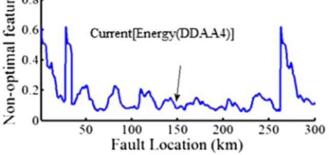
from the decomposed WPT coefficients. Thus the total feature matrix has 32 features (16 WPT coefficients2 features) which are then normalized between [1, +1]. As Daubechies works well in transient data, so it is taken for further analysis. Some of the WPT coefficients of fourth level are shown inFig. 8. Thereafter by using the forward feature selection method, 2 features, among 32 features as given in Table 1 are selected as best feature which can predict the target properly. Further, these two features as shown inTable 1is taken for the entire task of fault classification and location. The best feature plot and redundant feature plot are given inFigs. 9a–9c. It is noticed from Figs.9a and9b that the best feature gives a well defined path and for each fault distance it has some information, whereas fromFig. 9cwhich is a redundant feature plot, it is observed that the valuable information is lost as it shows an erratic path. During the training process optimal features are obtained.
Faulty current signal
Signal decomposition and feature
extraction by WPT
Best feature selection by forward
feature selection method and
normalization
Testing with the trained SVR model
SVR trained with the best feature set
Train and test data generation
Fig. 5.Flowchart of fault location technique.
Es Er Sending end/ Relaying end 300 km Fault Receiving end 400 kV voltage source
Fig. 6.Long transmission line under study.
Fig. 7a.Pre-fault and post-fault current signal for a-g fault.
Fig. 7b.Pre-fault and post-fault current signal for a-b fault.
Fig. 7c.Pre-fault and post-fault current signal for ab-g fault.
Further the trained SVM with the two optimal features are used for testing purpose. The train and test data are developed by taking into consideration a variety of simulation condition like the fault inception angle (h) and fault resistance (Rf) as shown inTable 2
for each 1 km of 300 km long transmission line in case of ten differ-ent categories of short circuit fault (a-g, b-g, c-g, a-b, b-c, c-a, ab-g, bc-g, ca-g, abc). FromTable 2it is noticed that the parameters to develop a train matrix is completely different from the test parameter, to make the planned method insensitive to parameter variations. Thus the total train data set consists of 240,000 data samples (10 types of fault resistance8 types of fault inception angle300 fault distances10 short-circuit fault). The test data Fig. 8.Some of the fourth level WPT coefficients.
Table 1
Best feature by WPT.
Signal type Feature (02) Best coefficient
Current Energy ADAD4
Entropy DDDD4
Fig. 9a.Optimal feature plot of coefficient ADAD4 of energy of current signal.
Fig. 9b.Optimal feature plot of coefficient DDDD4 of entropy of current signal.
Fig. 9c.Non-optimal feature plot.
Table 2
Parameters to develop, train and test data set.
Data-set Fault resistance (Rf) (inX) Fault inception angle (h) (in
degree) Train data 0, 1, 5, 10, 20, 40, 50, 70, 100, 150 10°, 20°, 30°, 40°, 50°, 60°, 70°, 80° Test data 2, 9, 25, 45, 65, 85, 110, 140 5°, 11°, 17°, 24°, 45°, 65°, 90°
matrix consists of 168,000 data samples (8 types of fault resis-tance7 types of fault inception angle300 fault distances10 types of fault). The test data set is taken as 70% of the train data set. The favorable values of SVM parameter are found by PSO, which is given inTable 3. The parameters of PSO used in this paper are reported inAppendix A. The test result of fault distance error is shown in the present work by box-plot. Box-plot is a graphical representation to show the error. In box-plot, the upper quartile indicates maximum error, the lower quartile shows minimum error, the area within the box indicates maximum error lying within the range of the box and the middle band shows mean or average error.
6. Simulation results
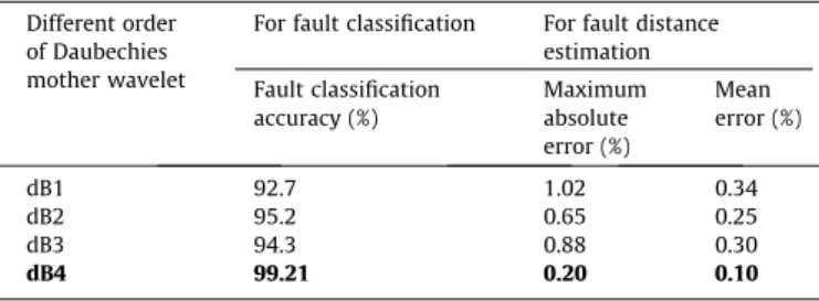
Initial testing has been carried out for fault classification and location to find the best order of Daubechies (dB) mother wavelet with the generated data sets in order to proceed the fault analysis task with the best one. An evaluation of the performance criterion for fault classification and location is made with four types of Dau-bechies mother wavelet which is given inTable 4. It is observed from Table 4that dB4 shows better fault classification accuracy (99.21%) and least fault location error (>0.21%) as compared to other mother wavelets. So dB4 is selected as mother wavelet for estimation of fault type and distance. Also, Daubechies wavelet has maximum number of vanishing moment. The wavelet’s ability to represent information in a signal is limited by vanishing moments. Vanishing moments for each wavelet is equal to half the number of coefficients. dB1 has one vanishing moment and encodes polynomial of one coefficient, dB2 has two vanishing moments and encodes linear and constant signal components, dB3 has three vanishing moments and encodes quadratic, linear and constant signal components. Due to the nature of the transient complex data and vanishing moments, results of dB3 is not linear. In Table 4, bold portions indicate that daubechies (dB4) gives highest fault classification accuracy and minimum fault location error. It is observed fromTable 5 that the average of classification accuracy is quite high (99.21%). The total test results of fault dis-tance estimation by the present discussed scheme is shown by Table 3
Best value of SVM by PSO.
SVM parameters For fault classification For fault distance estimation
For fault detection of the ground For phase fault detection
Kernel type Radial basis function Radial basis function Radial basis function
Gamma (g) 0.4 0.52 0.63
Cost (c) Not used Not used 12.4
Nu (nu) 0.5 0.45 0.15
Table 4
Comparison of mother wavelet test result. Different order
of Daubechies mother wavelet
For fault classification For fault distance estimation Fault classification accuracy (%) Maximum absolute error (%) Mean error (%) dB1 92.7 1.02 0.34 dB2 95.2 0.65 0.25 dB3 94.3 0.88 0.30 dB4 99.21 0.20 0.10 Table 5
Test results of fault classification.
Fault type No. of test data samples No. of test samples classified correctly No. of test samples misclassified Classification accuracy (%)
LG (a-g, b-g, c-g) 50,400 49,855 545 98.91
LL (a-b, b-c, c-a) 50,400 50,100 300 99.40
LLG (ab-g, bc-g, ca-g) 50,400 49,970 430 99.14
LLL (abc) 16,800 16,750 50 99.70
Total 168,000 166,675 1325 99.21
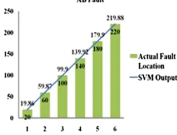
box-plot inFig. 10and further analyzed inTable 6. FromFig. 10, the observations noticed are presented inTable 6. It is observed from Table 6 that maximum absolute fault distance error is >0.21% and average error is also >0.11% and most of the error lies in the range 0.02–0.10%. The training time of the proposed fault classification and location method is 0.15 s. For a specific case of fault resistance (Rf= 45X), fault inception angle (h= 65°), six selected fault distance and four types of short circuit fault (a-g a-b, ab-g, abc),Fig. 11shows plots of the predicted output (SVM output) versus actual fault location. It is noticed fromFig. 11that >0.21% of maximum absolute fault distance error is there.
Separate investigation is also carried out to find a suitable sampling frequency (fs). In this regard, a series of high sampling frequencies (<30 kHz) and low sampling frequencies are consid-ered which is given inTable 7. It is shown fromTable 7that the data acquired in this paper give the best result for fault classifica-tion and locaclassifica-tion with 30 kHz sampling frequencies. So, it is considered for further fault analysis. Also in order to show the importance of PSO optimization technique based SVM, a compar-ison has been done in Table 8 with and without PSO for fault classification and fault location. It can be observed fromTable 8
that with optimized parameter of SVM with PSO in the proposed algorithm, fault classification accuracy (99.21%) and fault location error (>0.20%) is much better than without optimized parameter of SVM. The test results of fault location with and without opti-mized parameter of SVM in the proposed algorithm are shown in Figs. 10 and 12. For a particular fault inception angle (h= 24°) and fault resistance (Rf= 65X),Table 9shows some selected fault distances for four types of fault (a-g, a-b, ab-g, abc) which are
located very near to both the ends of the transmission line. It can be observed fromTable 9that all the errors are >0.21% and error very near to the source end is more. In order to show the superior-ity of SVM as fault classifier, it is compared with fault classifier’s like artificial neural network (ANN), probabilistic neural network (PNN) and adaptive neural fuzzy inference system (ANFIS) in
Table 10. The algorithm and other parameters as discussed in Section 5 remains the same for ANN, PNN and ANFIS for fault classification. The parameters of ANN, PNN and ANFIS used in this paper are given inAppendix. It can be observed fromTable 10that highest fault classification accuracy is provided by the proposed fault classifier i.e. SVC (99.21%).
InTable 8, bold portions shows that with optimized parameter of SVM with PSO, fault classification accuracy is more and fault location error is less as compared to without optimized parameter of SVM.
7. Background
In order to prove that the present discussed scheme for fault classification and distance estimation gives better accuracy as Table 6
Test results of fault location method. Fault type No. of samples Minimum absolute error (%) Maximum absolute error (%) Mean fault distance error (%) Range of the box (error range) a-g 16,800 0.00052 0.18 0.10 0.013–0.148 b-g 16,800 0.0027 0.17 0.08 0.022–0.17 c-g 16,800 0.002 0.19 0.10 0.02–0.18 a-b 16,800 0.00021 0.15 0.08 0.014–0.13 b-c 16,800 0.02 0.15 0.07 0.028–0.11 c-a 16,800 0.007 0.14 0.07 0.02–0.12 ab-g 16,800 0.001 0.20 0.10 0.006–0.19 bc-g 16,800 0.006 0.20 0.10 0.041–0.18 ca-g 16,800 0.0012 0.19 0.10 0.013–0.17 abc 16,800 0.0048 0.12 0.04 0.02–0.10
Fig. 11a.Actual versus predicted distance plot for AG fault.
Fig. 11b.Actual versus predicted distance plot for AB fault.
compared to other researcher’s work, a comparison has been made in Table 11. It can be seen fromTable 11that the present discussed scheme gives better accuracy for fault classification (99.21%) and minimum fault location error (>0.21%) as compared to methods used by other researchers. Also the training time of the proposed method is quite small (0.15 s). So, the proposed method is suggested for estimation of fault type and distance in a long transmission line.
Table 8
Test result with and without PSO.
For fault classification
For fault distance estimation Fault classification accuracy (%) Maximum absolute error (%) Mean error (%) With optimized parameter of SVM
with PSO
99.21 0.20 0.10
Without optimized parameter of SVM
95.01 0.32 0.22
Fig. 12.Box plot of test results for ten types of fault without PSO.
Table 9
Fault location test results for distances very near to source end of transmission line. Actual fault location (km) Absolute error (%)
AG fault AB fault ABG fault ABC fault
2 0.19 0.15 0.20 0.12 4 0.18 0.14 0.18 0.11 6 0.17 0.11 0.17 0.10 8 0.15 0.10 0.16 0.09 294 0.17 0.13 0.18 0.09 296 0.18 0.14 0.19 0.10 298 0.19 0.14 0.20 0.11 Table 10
Comparison of different fault classifiers.
Fault classifier Classification accuracy (%)
ANN 96
PNN 97
ANFIS 89
Proposed one (SVC) 99.21
Table 11
Comparison of different methods.
Schemes Fault classification Fault location
error (%) No. of test samples Classification accuracy (%) Method in[28] – – <0.30 Method in[48] 28,800 99.11 <0.45 Method in[49] 200 97.2 – Method in[50] – – <0.90 Method in[51] – – <1.0 Proposed method 168,000 99.21 >0.21 ES Er Sending end Fault Voltage Source-1 Voltage Source-2 TCSC 150 km 150 km
Fig. 13a.TCSC based transmission line under study. Fig. 11d.Actual versus predicted distance plot for ABC fault.
Table 7
Test results with different sampling frequencies.
Sampling frequency (kHz) Fault classification Fault location error (%) Classification accuracy (%) 0.1 93.5 <0.9 0.3 90.7 <1.0 50 92.4 <1.5 100 80.5 <2.7 Proposed method 99.21 >0.21 Capacitor (C) Inductor (L) Thyristor pairs MOV Triggered air gap Fig. 13b.TCSC details.
8. Fault classification and location with TCSC based transmission line
Fault classification and location of a 300 km transmission line with 400 kV source at both ends and a thyristor controlled series capacitor (TCSC) placed at the middle is discussed in this section. The model under study is as shown inFig. 13aand its detailed parameters are given inAppendix A. InFig. 13a,EsandErindicates front and rear end ideal voltage sources and the TCSC consists of an antiparallel connection of thyristors in each phase and a series combination of a reactor in parallel with a capacitor. A metal oxide varistor (MOV) with a parallel air gap arrangement protects the capacitor from overvoltage which is shown inFig. 13b. The protec-tion level of the MOV was adjusted to 721.81 kV based on minimal voltage across the capacitor which is 2.5 times when a standard current of 2 kA is flowing through it[35]. Post fault single cycle sending end current signal is acquired to classify and locate the ten types of short circuit fault (a-g, b-g, c-g, a-b, b-c, c-a, ab-g, bc-g, ca-g, abc) in the transmission line under study with a sam-pling frequency of 30 kHz. The same technique for fault classifica-tion and locaclassifica-tion as proposed in Secclassifica-tion5is implemented in this section. The other parameters of WPT, SVM and FFS method are the same as mentioned in Section5. Here, seven optimal features are selected by FFS from a total of 32 feature which is shown in
Table 12. One of the optimal and non-optimal feature plot is shown in Figs.14aand14brespectively in order to verify that optimal fea-ture gives a distinct path from which information can be extracted whereas non-optimal feature is random and unpredictable in nat-ure. The parameters to generate the train and test data set are the same as mentioned inTable 2of Section5. The test results of fault classification are given inTable 13and it can be observed that fault classification accuracy for all test cases is 98.36%. The test results of Table 12
Best feature in case of TCSC based transmission system by FFS. Signal type Feature (07) Best coefficient
Current Energy AAAA4, ADAD4, AADA4
Entropy ADDA4, AADD4, DADA4, DDDA4
Fig. 14a.Optimal feature plot for TCSC based transmission line.
Fig. 14b.Non-optimal feature plot for TCSC based transmission line.
Table 13
Test results of fault classification for TCSC based transmission line.
Fault type No. of test data samples No. of test samples classified correctly No. of test samples misclassified Classification accuracy (%)
LG (a-g, b-g, c-g) 50,400 49,392 1008 98.00
LL (a-b, b-c, c-a) 50,400 49,745 655 98.70
LLG (ab-g, bc-g, ca-g) 50,400 49,443 957 98.10
LLL (abc) 16,800 16,673 127 99.24
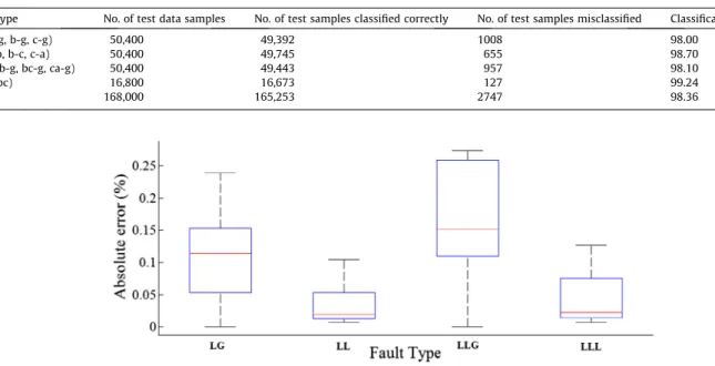
Total 168,000 165,253 2747 98.36
Fig. 15.Test results of fault location of TCSC based transmission line. Table 14
Test results of fault location for TCSC based transmission line.
Type of fault No. of test data samples Minimum absolute error (%) Maximum absolute error (%) Mean error (%) Range of the box (%)
LG (a-g, b-g, c-g) 50,400 0.00048 0.24 0.11 0.05–0.15
LL (ab, bc, ca) 50,400 0.006 0.10 0.02 0.01–0.05
LLG (ab-g, bc-g, ca-g) 50,400 0.0005 0.27 0.15 0.10–0.25
fault location for a particular case of fault inception angle (h= 45°) and fault resistance (Rf= 85X) is shown as box-plot inFig. 15. The analysis of Fig. 15 is given in Table 14 from which it can be observed that maximum absolute error is >0.28% and mean error is >0.15% which is acceptable.
In Table 14, bold portions shows that LG fault has minimum absolute error among all other faults (LL, LLG and LLL) and LLG fault has maximum absolute error and maximum mean error as compared to their faults (LG, LL, LLL).
9. Conclusion
Support vector machine based estimation of fault type and distance scheme in a long transmission line is proposed. For ten types of short circuit fault event, the proposed technique gives quick, correct and robust fault classification and location assess-ment of the collected one cycle post fault current signal. The uniqueness of the proposed technique is that it uses transient data to analyze the fault, a large number of features are collected by wavelet packet transform, forward feature selection method is applied to remove redundant features thereby enhancing the prediction accuracy, optimized value of support vector machine is used, variety of simulation conditions are considered to develop train and test data matrix and the simulation condition to develop test data matrix is made totally apart from the train one to make the proposed technique insensitive to parameter variations. The simulation result shows maximum fault classification accuracy (99.21%) and minimal fault position error (>0.21%) as compared to schemes proposed by other researchers. Also the training time is small (0.15 s) with SVM. The proposed method is also tested with long transmission line having TCSC placed in the middle. Simulation results of TCSC based model give >0.29% fault location error and fault classification accuracy of 98.36%.
Appendix A.
A.1. Parameters of the system under study
(i) Receiving and sending end voltage source parameter[35]: Positive sequence impedance (Z1): 1.31 +j16.0X. Zero sequence impedance (Z0): 2.22 +j27.6X. Frequency of the system: 50 Hz.
(ii) Parameter of long transmission line[35]: Length: 300 km, voltage: 400 kV.
Impedance of positive sequence = 8.15 +j94.5X. Impedance of zero sequence = 92.5 +j308X. Positive sequence capacitance = 14 nF/km. Zero sequence capacitance = 7.5 nF/km. A.2. Details of TCSC parameter[35]
L= 61.9 mH,C= 21.977
l
F.A.3. Particle swarm optimization parameters
c1 = 4, c2 = 4, particle size = 50, No. of iteration = 1000. wmin = 0.5, wmax = 0.9.
A.4. Parameters of ANN
Parameters of ANN is given inTable A.1.
A.5. Parameters of PNN and ANFIS
Kernel function used in PNN: Radial basis function.
Spread factorð
r
Þ ¼0:025ANFIS generates a Sugeno-type fuzzy inference system (FIS) using subtractive clustering technique with a radius of 0.5. References
[1]R. Das, D. Novosel, Review of fault location techniques for transmission and sub-transmission lines, in: Proc. 54th Annual Georgia Tech Protective Relaying Conf., 2000.
[2]M.E. Hawary, Electrical Power Systems, IEEE press, 1995. pp. 469–536. [3]M.M. Saha, J. Izykowski, E. Rosolowski, Fault Location on Power Networks,
Springer Pub., 2010.
[4]Y. Tang, H.F. Wang, R.K. Aggarwal, A.T. Johns, Fault Indicators in transmission and distribution systems, in: Proc. Int. Conf. Electric Utility Deregulation and Restructuring and Power Technologies 2000, City University, London, 2000, pp. 238–243. 4–7 April.
[5]D. Novosel, B. Bachmann, D.G. Hart, Y. Hu, M.M. Saha, Algorithms for locating faults on series compensated lines using neural network and deterministic methods, IEEE Trans. Power Delivery 11 (4) (1996) 1728–1736.
[6]T. Adu, A new transmission line fault locating system, IEEE Trans. Power Delivery 16 (4) (2001) 498–503.
[7]T. Takagi, Y. Yamakoshi, M. Yamaura, R. Kondou, T. Matsushima, Development of a new type fault locator using the one-terminal voltage and current data, IEEE Trans. Power Appl. Syst. PAS-101 (8) (1982) 2892–2898.
[8]L. Eriksson, M.M. Saha, G.D. Rockefeller, An accurate fault locator with compensation for apparent reactance in the fault resistance resulting from remote-end infeed, IEEE Trans. Power Appl. Syst. PAS-104 (2) (1985) 424–436. [9]S. Guobing, S. Jiale, G. Yaozhong, An accurate fault location algorithm for parallel transmission lines using one terminal data, Int. J. Electr. Power Energy Syst. 31 (2–3) (2009) 124–129.
[10] X. Lin, H. Weng, B. Wang, A generalized method to improve the location accuracy of the single-ended sampled data and lumped parameter model based fault locators, Int. J. Electr. Power Energy Syst. 31 (5) (2009) 201–205. [11]L. Eriksson, M.M. Saha, G.D. Rockefeller, An accurate fault locator with
compensation for apparent reactance in the fault resistance resulting from remote-end feed, IEEE Trans. Power Appl. Syst. PAS 104 (2) (1985) 1424–1436. [12]X. Dong, W. Kong, T. Cui, Fault classification and faulted phase selection based on the initial current travelling wave, IEEE Trans. Power Delivery 24 (2) (2009) 552–559.
[13]F. Chen, G. Qian, F. Wang, Study on traveling wave differential protection for series compensated line, J. Int. Council Electr. Eng. 1 (3) (2011) 359–366. [14]E.H. Shehab-Eldin, P.G. McLaren, Travelling wave distance protection-problem
areas and solutions, IEEE Trans. Power Delivery 3 (3) (1998) 894–902. [15]E.E. Ngu, K. Ramar, A combined impedance and travelling wave based fault
location method for multi-terminal transmission lines, Int. J. Electr. Power Energy Syst. 33 (10) (2011) 1767–1775.
[16]K. Liao, Z. He, X. Li, A fault location method based on traveling wave natural frequency used on ±800 kV UHVDC transmission lines, in: Proc. IEEE Electrical and Control Engineering (ICECE), 2011, pp. 5652–5655. 16–18 September. [17]M.J. Reddy, D.K. Mohanta, A comparative study of artificial neural network
(ANN) and fuzzy information system (FIS) approach for digital relaying of transmission line faults, AIML J. 6 (4) (2006) 1–7.
[18]M.J. Reddy, D.K. Mohanta, A wavelet-fuzzy combined approach for classification and location of transmission line faults, Int. J. Electr. Power Energy Syst. 29 (9) (2007) 669–678.
[19]A.K. Pradhan, A. Routray, S. Pati, D.K. Pradhan, Wavelet fuzzy combined approach for fault classification of a series compensated transmission line, IEEE Trans. Power Delivery 19 (4) (2004) 1612–1618.
[20] O.A.S. Youssef, Combined fuzzy logic wavelet based fault classification technique for power system relaying, IEEE Trans. Power Delivery 19 (2) (2004) 582–589.
[21]T. Dalstein, B. Kulicke, Neural network approach to fault classification for high speed protective relaying, IEEE Trans. Power Delivery 10 (2) (1995) 1002– 1011.
[22]S. Ekici, S. Yildirim, M. Poyraz, Energy and entropy based feature extraction for locating fault on transmission lines by using neural network and wavelet packet decomposition, Expert Syst. Appl. 34 (4) (2008) 2937–2944. Table A.1
Parameter details of ANN.
Network type Feed-forward back propagation network Training function Levenberg–Marquardt
Size of first hidden layer 40 Size of second hidden layer 04
Size of input layer Depends on the size of the optimal feature set Size of output layer 01
Train parameter goal 10e9
Performance function MSE(mean squared error)
[23]S. Ekici, S. Yildirim, M. Poyraz, A transmission line fault locator based on Elman recurrent networks, Appl. Soft Comput. 9 (1) (2009) 341–347.
[24]T. Bouthiba, Fault location in EHV transmission lines using artificial neural networks, Int. J. Appl. Math. Comput. Sci. 14 (1) (2004) 69–78.
[25]A.K. Pradhan, P.K. Dash, G. Panda, A fast and accurate distance relaying scheme using an efficient radial basis function neural network, Electr. Power Syst. Res. 60 (1) (2001) 1–8.
[26]H.K. Zadeh, M.R. Aghaebrahimi, A novel approach to fault classification and fault location for medium voltage cables based on artificial neural network, World Acad. Sci. Eng. Technol. 18 (2008) 1100–1103.
[27]S.R. Samantaray, P.K. Dash, G. Panda, Fault classification and location using HS-transform and radial basis function neural network, Electr. Power Syst. Res. 76 (9–10) (2006) 897–905.
[28]J. Sadeh, N. Hadjsaid, A.M. Ranjbar, R. Feuillet, Accurate fault location algorithm for series compensated transmission lines, IEEE Trans. Power Delivery 15 (3) (2000) 1027–1033.
[29]S. Ekici, Support vector machines for classification and locating faults on transmission lines, Appl. Soft Comput. 12 (6) (2012) 1650–1658.
[30]A.A. Yusuff, A.A. Jimoh, J.L. Munda, Fault location in transmission lines based on stationary wavelet transform, determinant function feature and support vector regression, Electr. Power Syst. Res. 110 (2014) 73–83.
[31]M.J. Reddy, P. Gopakumar, D.K. Mohanta, A novel transmission line protection using DOST and SVM, Eng. Sci. Technol. Int. J. 19 (2016) 1027–1039. [32]B.K. Panigrahi, V.R. Pandi, Optimal feature selection for classification of power
quality disturbances using wavelet packet-based fuzzy k-nearest neighbor algorithm, IET Gener. Transm. Distrib.3 (3) (2009) 296–306.
[33] <www.mathworks.in/help/wavelet/ug/wavelet-packets.html>.
[34] P. Ray, D. Mishra, Application of extreme learning machine for underground cable fault location, Int. Trans. Electr. Energy Syst. (2014),http://dx.doi.org/ 10.1002/etep.2032.25(7). Wiley.
[35]P. Ray, B.K. Panigrahi, N. Senroy, Hybrid methodology for fault distance estimation in series compensated transmission line, IET Gener. Transm. Distrib. 7 (5) (2013) 431–439.
[36]P. Luukka, Feature selection using fuzzy entropy measures with similarity classifier, Expert Syst. Appl. 38 (4) (2011) 4600–4607.
[37]O. Maron, A. Moore, The racing algorithm: model selection for lazy learners, Artif. Intell. Rev. 11 (1997) 193–225.
[38]L. Devroye, The uniform convergence of nearest neighbor regression function estimators and their application in optimization, IEEE Trans. Inf. Theory 24 (2) (1978) 142–151.
[39]A. Navot, L. Shpigelman, N. Tishby, E. Vaadia, Nearest neighbor based feature selection for regression and its application to neural activity, in: Proc. Int. Conf. Advances in Neural Information Processing Systems NIPS, 18, 2006, pp. 995– 1002.
[40]U.B. Parikh, B. Das, R. Maheshwari, Fault classification technique for series compensated transmission line using support vector machine, Int. J. Electr. Power Energy Syst. 32 (6) (2010) 629–636.
[41] en.wikipedia.org/wiki/Support_vector_machine.
[42]K. Schittkowski, Optimal parameter selection in support vector machines, J. Ind. Manage. Optim. 1 (4) (2005) 465–476.
[43] LIBSVM-A library for support vector machines (online). Available: <http:// www.csie.ntu.edu.tw/~cjlin/libsvm>.
[44] <http://scikit-learn.org/dev/auto_examples/svm/plot_rbf_parameters.html>. [45]I. Steinwart, On the optimal parameter choice form-support vector machines,
IEEE Trans. Pattern Anal. Mach. Intell. 25 (10) (2003) 1274–1284.
[46]P.K. Dash, A.K. Pradhan, G. Panda, A novel fuzzy neural network based distance relaying scheme, IEEE Trans. Power Delivery 15 (3) (2000) 902–907. [47]M. Akke, J.T. Thorp, Some improvements in the three-phase differential
equation algorithm for fast transmission line protection, IEEE Trans. Power Delivery 13 (1) (1998) 66–72.
[48]V. Malathi, N.S. Marimuthu, S. Baskar, K. Ramar, Application of extreme learning machine for series compensated transmission line protection, Eng. Appl. Artif. Intell. 24 (5) (2011) 880–887.
[49]P.K. Dash, S.R. Samantaray, G. Panda, Fault classification and section identification of an advanced series compensated transmission line using support vector machine, IEEE Trans. Power Delivery 22 (2007) 67–73. [50]S. Sahoo, P. Ray, B.K. Panigrahi, N. Senroy, A computational intelligence
approach for fault location in transmission lines, in: Proc. IEEE Conf. Power Electronics, Drives and Energy Systems (PEDES-2010), 2010, pp. 1–6. December 21–23.
[51]M.M. Saha, J. Izykowski, E. Rosolowski, B. Kasztenny, A new accurate fault locating algorithm for series compensated lines, IEEE Trans. Power Delivery 14 (3) (1999) 789–797.