A Clustering System for Dynamic Data Streams Based
on Metaheuristic Optimisation
Jia Ming Yeoh1, Fabio Caraffini1* , Elmina Homapour1 , Valentino Santucci2 and Alfredo Milani3
1 Institute of Artificial Intelligence, School of Computer Science and Informatics, De Montfort University, Leicester (UK); [email protected]; [email protected]; [email protected] 2 University for Foreigners of Perugia, Perugia (Italy); [email protected]
3 University of Perugia, Perugia (Italy); [email protected] * Correspondence: [email protected]
Version December 10, 2019 submitted to Mathematics
Abstract:This article presents OpStream, a novel approach to cluster dynamic data streams. The 1
proposed system displays desirable features, such as a low number of parameters, good scalability 2
capabilities to both high-dimensional data and numbers of clusters in the data set, and it is based on 3
a hybrid structure using deterministic clustering methods and stochastic optimisation approaches to 4
optimally centre the clusters. Similarly to other state-of-the-art methods available in the literature, 5
it uses “microclusters” and other established techniques, such as density-based clustering. Unlike 6
other methods, it makes use of metaheuristic optimisation to maximise performances during the 7
initialisation phase, which precedes the classic online phase. Experimental results show that 8
OpStream outperforms the state-of-the-art in several cases and it is always competitive against 9
other comparison algorithms regardless of the chosen optimisation method. Three variants of 10
OpStream, each coming with a different optimisation algorithm, are presented in this study. A 11
thorough sensitive analysis is performed by using the best variant to point out OpStream robustness 12
to noise and resiliency to parameters changes. 13
Keywords: dynamic stream clustering; online clustering; metaheuristics; optimisation; 14
population-based algorithms; density-based clustering; k-means centroid; concept-drift; 15
concept-evolution 16
1. Introduction 17
Clustering is the process of grouping homogeneous objects based on the correlation among 18
similar attributes. This is useful in several common applications that require the discovery of hidden 19
patterns among the collective data to assist decision making, e.g. bank transaction fraud detection [1], 20
market trend prediction [2,3], and network intrusion detection system [4]. Most traditional clustering 21
algorithms developed relies on multiple iterations of evaluation on a fixed set of data to generate the 22
clusters. However, in practical applications, these detection systems are operating daily, whereby 23
millions of input data points are continuously streamed indefinitely, hence imposing speed and 24
memory constraints. In such dynamic data stream environments, keeping track of every historical data 25
would be highly memory expensive and, even if possible, would not solve the problem of analysing 26
big data within the real-time requirements. Hence, a method of analysing and storing the essential 27
information of the historical data in a single pass is mandatory for clustering data streams. 28
In addition, dynamic data clustering algorithm needs to address two special characteristics that 29
often occurs in data streams which is known asconcept-driftandconcept-evolution[5]. Concept drift 30
refers to the change of underlying concepts in the stream as time progress, i.e. the change in the 31
relationship between the attributes of the object within the individual clusters. For example, customer 32
behaviour in purchasing trending products always changes in between seasonal sales. Meanwhile, 33
concept evolution occurs when a new class definition has evolved in the data streams, i.e. the number 34
of clusters has changed due to the creation of new clusters or deprecation of old clusters. This 35
phenomenon often occurs in the detection system whereby an anomaly has emerged in the data traffic. 36
An ideal data stream clustering algorithm should address these two main considerations to effectively 37
detect and adapt to changes in the dynamic data environment. 38
Based on recent literature, metaheuristics for black-box optimisation have been greatly adopted 39
in traditional static data clustering [6]. These algorithms have a general-purpose application domain 40
and often displays self-adaptive capabilities, thus being able to tackle the problem at hand, regardless 41
of its nature and formulation, and return near-optimal solutions. For clustering purposes, the so-called 42
“population-based” metaheuristic algorithms have been discovered to be able to achieve better global 43
optimisation results than their “single-solution” counterparts [7]. Amongst the most commonly used 44
optimisation paradigms of this kind, it is worth mentioning the established Differential Evolution (DE) 45
framework [8–10], as well as more recent nature-inspired algorithms from the Swarm Intelligence (SI) 46
field, such as the Whale Optimisation Algorithm (WOA) [11] and the Bat-inspired algorithm in [12], 47
here referred to as BAT. Although the literature is replete with examples of data clustering strategies 48
based on DE, WOA and BAT for the static domain, as e.g. those presented in [13–16], a little is done 49
for the dynamic environment due to the difficulties in handling data streams. The current state of 50
dynamic clustering is therefore unsatisfactory as it mainly relies on algorithms based on techniques, 51
such as density microclustering and density grid-based clustering, which requires the tuning of several 52
parameters to work effectively [17]. 53
This paper presents a methodology for integrating metaheuristic optimisation into data stream 54
clustering, thus maximising the performance of the classification process. The proposed model does not 55
require specifically tailored optimisation algorithms to function, but it is a rather general framework to 56
use when highly dynamics streams of data have to be clustered. Unlike similar methods, we do not 57
optimise parameters of a clustering algorithm but use metaheuristic optimisation in its initialisation 58
phase, in which the first clusters are created, by finding the optimal position of their centroids. This is 59
a key step as the grouped points are subsequently processed with the method in [18] to form compact, 60
but informative,microclusters. Hence, by creating the optimal initial environment for the clustering 61
method, we make sure that the dynamic nature of the problem will not deteriorate its performances. It 62
must be noted that microclusters are lighter representations of the original scenario which are stored 63
to preserve the “memory” of the past classifications. These play a major role since aid subsequent 64
clustering processes when new data streams are received. Thus, by a non-optimal microclusters store 65
in memory can have catastrophic consequences in terms of classification results. In this light, our 66
original use of the metaheuristic algorithm finds its purpose and results confirm the validity of our 67
idea. thee proposed clustering scheme efficiently track changes and spot patterns accordingly. 68
The remainder of this paper has the following structure: 69
• section2discusses the recent literature and briefly explains the logic behind the leading data 70
stream clustering algorithms; 71
• section 3 establishes the motivations and objectives of this research and presents the used 72
Metaheuristic Optimisation methods, the employed performance metrics, and the considered 73
data sets for producing numerical results; 74
• section4gives a detailed description of each step involved in the proposed clustering system, 75
clarifies its working mechanism and show methodologies for its implementation; 76
• section 5 describes the performance metrics used to evaluate the system and provides 77
experimental details to reproduce the presented results; 78
• section6presents and comments on the produced results, including comparison among different 79
variants of the proposed system, over several evaluation metrics; 80
• section7outlines a thorough analysis of the impact of the parameter setting for the optimisation 81
algorithm on the overall performance of the clustering system; 82
• section8summarises the conclusions of this piece of research. 83
2. Background 84
There are two fundamentals aspects to take into consideration in data stream clustering, namely 85
concept-driftandconcept-evolution. The first aspect refers to the phenomenon when the data in the 86
stream undergoes changes in the statistic properties of the clusters with respect to the time [19,20] 87
while the second to the event when there is an unseen novel cluster appearing in the stream [5,21]. 88
Time window models are deployed to handle concept-drift in data streams. These are usually 89
embedded into clustering algorithms to control the quantity of historical information used in analysing 90
dynamic patterns. Currently, there are four predominant window models in the literature [22]: 91
• the “damped time window” model, where historical data weights are dynamically adjusted by 92
fixing a rate of decay according to the number of observations assigned to it [23]; 93
• the “sliding time window” model, where only the most recent past data observations are 94
considered with a simple First-In-First-Out (FIFO) mechanism as in [24]; 95
• the “landmark time window” model, where the data stream is analysed in batches by 96
accumulating data in a fixed-width buffer before being processed; 97
• the “tilted time window” model, where granularity level of weights gradually decreases as data 98
point gets older. 99
As for concept-evolution, most of the existing data stream clustering algorithms are designed 100
following a two-phases approach, i.e. consisting of anonlineclustering process followed by anoffline 101
one, which was first proposed in [25]. In this work, the concept of microclusters was also defined 102
to design the so-called “CluStream” algorithm. This method forms microclusters having statistical 103
features representing the data stream online. Similar microclusters are then merged into macro-clusters, 104
keeping only information related to the centre of the densest region. This is performed offline, upon 105
user request, as it comes with information losses since merged clusters can no longer be split again to 106
obtain the original ones. 107
In terms of online microclustersing, most algorithms in the literature are distance-based [22,26,27], 108
whereby new observations are either merged to existing microclusters or form new microclusters 109
based on a distance threshold. The earliest form of distance-based clustering strategy is the process 110
of extracting information about a cluster into the form of a Clustering Feature (CF) vector. Each CF 111
usually consists of three main components: 1) a linear combination of the data points referred to as 112
Linear Sum vector−LS; 2) a vector→ −→SS whose components are the Squared Sums of the corresponding 113
data points components; 3) the number N of points in a cluster. 114
As an instance, the popular CluStream algorithm in [25] makes use of CF and the tilted time 115
window model. During the initialisation phase, data points are accumulated to a certain amount before 116
being converted into some microclusters. On the arrival of new streams, new data are merged with the 117
closest microclusters if their distance from the centre of the data point to the centre of the microclusters 118
is within a given radius (i.e.e-neighbourhood method). If there is no suitable microclusters within this 119
range, a new microclusters is formed. When requested, the CluStream uses the k-means algorithm 120
[28] to generate macro-clusters from microclusters in its offline phase. It also implements an ageing 121
mechanism based on timestamps to remove outdated clusters from its online components. 122
Another state-of-the-art algorithm, i.e. DenStream, is proposed in [18] as an extension of 123
CluStream using the damped time window and a novel clustering strategy named “time-faded 124
CF”. DenStream separates the microclusters into two categories: the potential core microclusters 125
(referred to asp-microclusters) and the outlier microclusters (referred to aso-microclusters). Each entry 126
of the CF is subject to a decay function that gradually reduces the weight of each microclusters at 127
a regular evaluation interval period. When the weight falls below a threshold value, the affected 128
p-microclustersare degraded to theo-microclusters, and they are removed from theo-microclustersif 129
the weights deteriorates further. On the other hand,o-microclustersthat have their weights improved 130
are promoted to p-microclusters. This concept allows new and old clusters to gradually form online, 131
so addressing the concept evolution issue. In the offline phase, only thep-microclustersare used for 132
generating the final clusters. Similar p-microclusters are merged employing a density-based approach 133
based on thee-neighbourhood method. Unlike other commonly used methods, in this case clusters 134
can assume an arbitrary shape and no a-priori information is needed to fox the number of clusters. 135
An alternative approach is given in [29], where the proposed STREAM algorithm does not 136
store CF vectors but directly compute centroids on-the-flight. This is done by solving the “k-Median 137
clustering” problem to identify the centroids ofKclusters. The problem is structured in a form whereby 138
the distance from data points to its closest cluster has associated costs. Using this framework, the 139
clustering task is defined as a minimisation problem to find the number and position of centroids 140
that yield the lowest costs. To process indefinite length of streaming data, landmark time window is 141
used to divide the streams intonbatches of data, and theK-median problem solving is performed on 142
each chunk. Although the solution is plausible, the algorithm is evaluated to be time-consuming and 143
memory expensive in processing streaming data. 144
The OLINDDA method proposed in [30] extends the previously described centroid approach 145
by integrating thee-neighbourhood concept. This is used to detect drifting and new clusters in the 146
data stream, with the assumption that drift changes occur within the existing cluster region whilst 147
new clusters form outside the existing cluster region. The downside of the centroid approach is 148
that the number ofKcentroids needs to be known a-priori, which is problematic in a dynamic data 149
environment. 150
There is one shortcoming for the two-phases approach, i.e. the ability to track changes in the 151
behaviour of the clusters is linearly proportional to the frequency of requests for the offline component 152
[31]. In other words, the higher the sensitivity to changes, the higher the computational cost. To 153
mitigate these issues, an alternative approach has been explored by researchers to merge these two 154
phases into a single online phase. FlockStream [32] deploys data points into a virtual mapping of a 155
two-dimensional grid, where each point is represented as an agent. Each agent navigates around the 156
virtual space according to a model mimicking the behaviour of flocking birds, as done in the most 157
popular SI algorithms, e.g. those in [33–35]. The agent behaviour is designed in a way such that similar 158
(according to a given metric) birds will move in the same direction as its closest neighbours, forming 159
different groups of the flock. These groups can be seen as clusters, thus eliminating the need for a 160
subsequent offline phase. 161
MDSC [36] is another single-phase method exploiting the SI paradigm inspired by the 162
density-based approached introduced in DenStream. In this method, the Ant Colony Optimisation 163
(ACO) algorithm [37] is used to optimally group similar microclusters during the online phase. In 164
MDSC, a customisede-neighbourhood value is assigned to each cluster to enable “multi-density” 165
clusters to be discovered. 166
Finally, it is worth mentioning the ISDI algorithm in [38], which is equipped with a windowing 167
routine to analyse and stream data from multiple sources, a timing alignment method and a 168
deduplication algorithm. This algorithm is designed to deal with data streams coming from different 169
sources in the Internet of Things (IoT) systems and can transform multiple data streams, having 170
different attributes, into cleaner data sets suitable for clustering. Thus, it represents a powerful tool 171
allowing for the use of streams classifiers, as a.g. the one proposed in this study, in IoT environments. 172
3. Motivations, Objectives and Methods 173
Clustering data streams is still an open problem with room of improvement [39]. Increasing the 174
classification efficiency in this dynamic environment has a great potential in several application fields, 175
from intrusion detection [40] to abnormalities detection in patients physiological streams data [41]. In 176
this light, the proposed methodology draws its inspiration from key features of the successful methods 177
listed in section2, with the final goal of improving upon the current state-of-the-art. 178
A hybrid algorithm is then designed by employing, along with standard methods as e.g. CF 179
vectors and the landmark time windows model, modern heuristic optimisation algorithms. Unlike 180
similar approaches available in the literature [37,42,43], the optimisation algorithm is here used during 181
the online phase to create optimal conditions to the offline phase. This novel approach is described in 182
details in section4. 183
To select the most appropriate optimisation paradigm, three widely used algorithms, i.e. WOA, 184
BAT and DE, were selected from the literature and compared between them. We want to clarify that 185
the choice of using three metaheuristic methods, rather than other exact or iterative techniques, was 186
made to be able to deal with ch alleging characteristics of the optimisation problem at hand, e.g. the 187
dimensional of the problem can vary according to the data set, the objective functions is highly non 188
linear and not differentiable, which make them not applicable or time-inefficient. 189
A brief introduction of the three selected algorithms is given below in section3.1. Regardless of 190
the specific population-based algorithm used for performing the optimisation step, each candidate 191
solution must be encoded as ann-dimensional real-valued vector representing theKcluster centres for 192
initialising the following density-based clustering method. 193
Two state-of-the-art deterministic data stream clustering algorithms, namely DenStream and 194
CluStream, are also included in the comparative analysis to further validate the effectiveness of the 195
proposed framework. 196
The evaluation methodology employed in this work consists in running classification experiments 197
over the data sets in section3.2and measuring the obtained performances through the metrics defined 198
in section3.3. 199
3.1. Metaheuristic Optimisation methods 200
This section gives details on the implementation of the three optimisation methods used to test 201
the proposed system. 202
3.1.1. The Whale Optimization Algorithm 203
The WOA algorithm is a swarm-based stochastic metaheuristic algorithm inspired by the hunting 204
behaviour of humpback whales [11]. It is based on a mathematical model updated by iterating the 205
three search mechanisms described below: 206
• the “shrinking encircling prey” mechanism is exploitative and consists in moving candidate 207
solutions (i.e. the whales) in a neighbourhood of a the current best solution in the swarm (i.e. the 208
prey solution) by implementing the following equation: 209 −→x(t+1) =−→x best(t)− −→ A ∗−→Dbest with −→ A =2−→a ∗ −→r − −→a −→ Dbest =2−→r ∗ −−→xbest(t)− −→x(t) (1)
where: 1)−→a is linearly decreased from 2 to 0 as iterations increase (to represent shrinking as 210
explained in [7]); 2)−→r is a vector whose components are randomly sampled from[0, 1](tis the 211
iteration counter); 3) the “∗” notation indicates the pairwise products between two vectors. 212
• the “spiral updating position” mechanism is also exploitative and mimics the swimming pattern of humpback whales towards the prey in a helix-shaped form through equations (2) and3:
−→x (t+1) =ebl∗cos(2 πl)∗ −→ d + −→x best(t) (2) with −→ d = −→x best(t)− −→x(t) (3)
wherebis a constant value for defining the shape of logarithmic spiral;lis a random vector in 213
[−1, 1]; the “|. . .|” symbol indicates the absolute value of each component of the vector; 214
• the “search for prey” mechanism is exploratory and uses a randomly selected solution−→xrand as “attractor” to move candidate solutions towards unexplored areas of the search space, and possibly away from local optima, according to equations (4) to (5):
−→x(t+1) =−→x rand(t)− −→ A∗−→D+rand (4) with −→ Drand= 2 −→a ∗ −→r ∗ −−→x rand(t)− −→x . (5)
The reported equations implement a search mechanism which mimics movements made by 215
whales. Mathematically, it is easier to understand that some of them refer to explorations moves across 216
the search space, while others are exploitation move to refine solutions within their neighbourhood. 217
To have more information on the metaphor inspiring this equations, their formulations and their 218
role in driving the research within the algorithm framework, one can see the survey article in [6]. A 219
derailed scheme describing the coordination logic of the three previously described search mechanism 220
is reported in algorithm1. 221
Algorithm 1WOA pseudocode
1: Generate initial whale positionsxi, wherei=1, 2, 3, . . . ,NP
2: Compute fitness of each whale solution and identifyxbest 3: whilet<max iterationsdo
4: fori=1, 2, . . . ,NPdo 5: Updatea,A,C,l,p
6: ifp<0.5then 7: if|A|<1then
8: Update position of current whalexiusing equation1
9: else if|A| ≥1then
10: xrand←random whale agent
11: Update position of current whalexiwith equation4
12: end if
13: else ifp≥0.5then
14: Update position of current whalexiwith equation2
15: end if
16: end for
17: Calculate new fitness values 18: UpdateXbest
19: t=t+1 20: end while 21: Returnxbest
With reference to algorithm1, the initial swarm is generated by randomly sampling solutions in 222
the search; the best solution is kept up to date by replacing it only when an improvement on the fitness 223
value occurs; the optimisation process lasts for a prefixed number of iterations, here indicated with 224
max budget; he probability of using the shrinking encircling rather than the spiral updating mechanism 225
is fixed at 0.5. 226
3.1.2. The BAT Algorithm 227
The BAT algorithm is a swarm-based searching algorithm inspired from the echolocation abilities 228
of bats [12]. Bats use sound wave emission to generate echo that measures the distance of its prey 229
based on the loudness and time difference of the echo and sound wave. To reproduce this system and 230
exploit it for optimisation purposes, the following perturbation strategy must be implemented: 231
vi(t+1) =vi(t) + (xi(t)−xbest)·fi (7)
xi(t+1) =xi(t) +vi(t) (8)
wherexi is the position of the candiate solution in the search space (i.e. the bat), vi is its velocity, 232
fi is referred to as “wawes frequency” factor and βis a random vector in [0, 1]n (where n is the 233
dimentionality of the problem). fminand fmax represent the lower and upper bounds of the frequency 234
respectively. Typical values are within 0 and 100. When the bat is close to the prey (i.e. current best 235
solution), it gradually reduces the loudness of its sound wave while increasing the pulse rate. The 236
pseudocode depicted in algorithm2shows the the working mechanism of the BAT algorithm. 237
Algorithm 2BAT pseudocode
1: Generate initial batsXi(i=1, 2, 3, . . . ,NP) and their velocity vectorsvi
2: Compute fitness values and findxbest 3: Initialise pulse frequency fiatxi
4: Initialise pulse rateriand loudnessAi
5: whilet<max iterationsdo 6: fori=1, 2, 3, . . . ,NPdo
7: xnew←movexito a new position with equations6–8
8: end for
9: fori=1, 2, 3, . . . ,NPdo 10: ifrand()>rithen
11: xnew←xbestadded with a random
12: end if
13: ifrand()<Aiand f(xnew)improvedthen
14: Xi←xnew
15: Increaseriand decreaseAi
16: end if 17: end for 18: Updatexbest 19: t=t+1 20: end while 21: Returnxbest
To have more detailed information on the equations used to perturb the solutions within the 238
search space in the BAT algorithm, we suggest reading [44]. 239
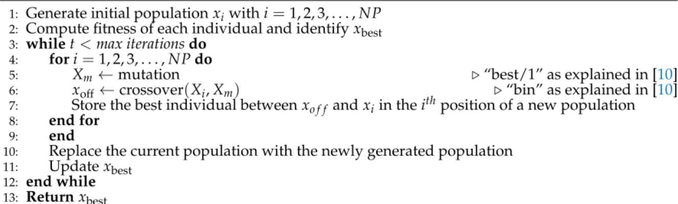
3.1.3. The Differential Evolution 240
The Differential Evolution (DE) algorithms are efficient metaheuristics for global optimisation 241
based on a simple and solid framework, first introduced in [45], which only requires the tuning of 242
three parameters, namely the scale factorF∈[0, 2], the crossover ratioCR∈[0, 1]and the population 243
sizeNP. As shown in algorithm3, despite usingcrossoverandmutationoperators, which are typical 244
of evolutionary algorithms, it does not require any selection mechanism as solutions are perturbed 245
one at a time by means of the 1-to-1 spawning mechanising from the SI field. Several DE variants can 246
be obtained by using different combination of crossover and mutation operators [46]. The so-called 247
“DE/best/1/bin” scheme is adopted in this study, which employs thebestmutation strategy and the 248
binomialcrossover approach. Pseudocode and other details regarding these operators are available in 249
[10]. 250
Algorithm 3DE pseudocode
1: Generate initial populationxiwithi=1, 2, 3, . . . ,NP
2: Compute fitness of each individual and identifyxbest 3: whilet<max iterationsdo
4: fori=1, 2, 3, . . . ,NPdo
5: Xm←mutation .“best/1” as explained in [10]
6: xoff←crossover(Xi,Xm) .“bin” as explained in [10]
7: Store the best individual betweenxo f f andxiin theithposition of a new population
8: end for
9: end
10: Replace the current population with the newly generated population 11: Updatexbest
12: end while 13: Returnxbest
3.2. Datasets 251
Four synthetic data sets were generated using the built-in stream data generator of the “Massive 252
Online Analysis” (MOA) software [47]. Each synthetic data set represents different data streaming 253
scenarios with varying dimensions, clusters numbers, drift speed and frequency of concept evolution. 254
These data sets are: 255
• the5C5Cdata set, which contains low dimensional data with a low rate of data changes; 256
• the5C10Cdata set, which contains low dimensional data with a high rate of data changes; 257
• the10D5Cdata set, which is a5C5Cvariant containing high dimensional data; 258
• the10D10Cdata set, which is a5C10Cvariant containing high dimensional data. 259
Moreover, theKDD-99data set [48], containing real network intrusion information, was also 260
consdered in this study. It must be highlighted that the originalKDD-99data set contains 494021 data 261
entries representing network connections generated in military network simulations. However, only 262
10% of the entries were randomly selected for this study. Each data entry contains 41 features and 1 263
output column to distinguish the attack connection from the normal network connection. The attacks 264
can be further classified into 22 attack types. Streams are obtained by reading each entry of the data set 265
sequentially. 266
Details on the five employed data sets are given in table1. 267
Table 1.Name and Description of Synthetic Datasets and Real Dataset
Name Dimension Clusters No. Samples Drift Speed Event Frequency Type
5D5C 5 3–5 100,000 1,000 10,000 Synthetic
5D10C 5 6–10 100,000 5,000 10,000 Synthetic
10D5C 10 3–5 100,000 1,000 10,000 Synthetic
10D10C 10 6–10 100,000 5,000 10,000 Synthetic
KDD–99 41 2–23 494,000 Not Known Not Known Real
3.3. Performance Metrics 268
To perform an informative comparative analysis three metrics were cherry-picked from the data 269
stream analysis literature [42,43]. These are referred to asF-Measure,PurityandRand-Index[49]. 270
Mathematically, these metrics are expressed with the following equations: 271 F-Measure= 1 k k
∑
i=1 ScoreCi (9) Purity= 1 k k∑
i=1 PrecisionCi (10)Rand-Index= True Positive+True Negative
All Data Instances (11)
where PrecisionCi = Visum nCi (12) ScoreCi =2· PrecisionCi·RecallCi PrecisionCi +RecallCi (13) RecallCi = Visum Vitotal (14) and 272
• Cis the solution returned by the clustering algorithm (i.e. the number of clustersk); 273
• Ciis the theithcluster (i={1, 2, . . . ,k}); 274
• Viis the class label with the highest frequency inCi; 275
• Visumis the number of instances labelled withViinCi; 276
• Vitotalis the total number ofViinstances identified in the totality of clusters returned by the 277
algorithm. 278
F-Measure represents the harmonic mean of the Precision and Recall scores, where the best value 279
of 1 indicates ideal Precision and Recall, while 0 is the worst scenario. 280
Purity is used to measures the homogeneity of the clusters. Maximum purity is achieved by the 281
solution when each cluster only contains a single class. 282
Rand-Index computes the accuracy of the clustering solution from the actual solution, based on 283
the ratio of correctly identified instances among all the instances. 284
4. The Proposed System 285
This article proposes “OpStream”, an Optimised Stream Clustering Algorithm. This clustering 286
framework consists of two main parts: theinitialisationphase and theonlinephase. 287
During the initialisation phase, a numberλof data points are accumulated through a landmark 288
time window, the unclassified points are initialised into groups of clusters via the centroid approach, 289
i.e. generatingKcentroids of clusters among the points. 290
In the initialisation phase, the landmark time window is used to collect data points which are 291
subsequently grouped into clusters by generatingKcentroid. The latter, are generated from by solving 292
K-centroid cost optimisation problems with fast and reliable metaheuristic for optimisation. Hence, 293
their position is optimal and lead to high-quality predictions. 294
Next, during the online phase, the clusters are maintained and updated using the density-based 295
approach, whereby incoming data points with similar attributes (i.e. according to thee-neighbourhood 296
method) form dense microclusters in between two data buffers, namely p-microclusters and 297
o-microclusters. These are converted into microclusters with CF information to store a “light” version 298
previous scenarios in this dynamic environment. 299
In this light, the proposed framework is similar to advanced single-phase methods. Howevere, it 300
requires a preliminary optimisation process to boost its classification performances. 301
Three variants of OpStream are tested by using the three metaheuristic optimisers described in 302
section3. These stochastic algorithms (as the optimisation process is stochastic) are compared against 303
the two DenStream and CluStream state-of-the-art deterministic stream clustering algorithms. 304
The following sections describe each step of the OpStream algorithm. 305
4.1. The Initialisation Phase 306
This step can be formulated as a real-valued global optimisation search problem and addressed 307
with metaheuristic of black-box optimisation. To achieve this goal, a cost function must be designed 308
to allow for the individualisation of the optimal position of the centroid of a cluster. These processes 309
have to be iteratedKtimes to then formKclusters by grouping data according to their distance from 310
the optimal centroids. 311
The formulation of the cost function plays a key part. In this research, the “Cluster Fitness” (CF) function from [50] was chosen as its maximisation leads to a high intra-cluster distance, which is desirable. Its mathematical formulation, for theκth(κ=1, 2, 3, . . .K) cluster, is given below
CFκ = 1 K K
∑
κ=1 Sκ (15)from where it can be observed that it is computed by averaging theKclusters’ Silhouettes “Sκ”. These,
represents the average dissimilarity of all the points in the cluster, and are calculated as follows
Sκ = 1 nki
∑
∈Cκ βi−αi max{αi,βi} (16)whereαiandβiare the “Inner Dissimilarity” and the “Outer Dissimilarity” respectively. 312
The former value measures the average dissimilarity between a data pointiand other data points in its own clusterCκ∗. Mathematically, this is expressed as:
αi = 1 (nk∗−1)
∑
j∈Cκ∗ j6=i dist(i,j) (17)with dist(i,j)being the Euclidean distance between the two points, andnk∗ is the total number of 313
points in clusterCκ∗. The lower the value, the better the clustering accuracy.
314
The latter value measures the minimum distance between a data pointito the centre of all clusters, excluding its own clusterCκ∗. Mathematically, this is expressed as:
βi = min κ=1,...,K k6=κ∗ 1 nk j
∑
∈C κ k6=κ∗ dist(i,j) ! (18)wherenk∗is the number of points in clusterCκ∗. The higher the value, the better the clustering. 315
These two values are contained in [−1, 1], whereby 1 indicates ideal case and −1 the most 316
undesired one. 317
A similar observation can be done for the fitness function CFκ [50]. Hence, the selected
318
metaheuristics have to be set-up for a maximisation problem. This is not an issue since every 319
real-valued problem of this kind can be easily maximised with an algorithm designed for minimisation 320
purposes by simply timing the fitness function by−1, and vice-versa. 321
Regardless of the dimensionality of the problemn, which depends on the data set (as shown in 322
table1), all input data are normalised within[0, 1]. Thus, the search space for all the optimisation 323
process is the hyper-cube defined as[0, 1]n. 324
4.2. The Online Phase 325
Once the initial clusters have been generated, by optimising the cost function formulated in section 326
4.1, clustered data points must be converted into microclusters. This step requires the extraction of CF 327
vectors. Subsequently, a density-based approach is used to cluster data stream online. 328
4.2.1. microclusters Structure 329
In OpStream, each CF must contain four components, i.e. CF= [N,−LS,→ −→SS, timestamp], where 330
• N∈Nis the number of data points in the microclusters;
• −LS→∈Rnis the linear sum of the data points in the microcluster, i.e. −→ LS= N
∑
i=1 −→x i;• −→SS∈Rnis the squared sum of the data points in the microclusters i.e. −→ SS[j] = N
∑
i=1 −→ xi[j] 2 ; j=1, 2, 3, . . . ,n• timestamp indicates when the microclusters was last updated and it is needed to implement the ageing mechanism, used to remove outdated microclusters while new data accumulated in the time window are available, defined via the following equation
age=T−timestamp (19)
where T is the current time-stamp in the stream a threshold, referred to as β, is used to 332
discriminate between suitable and outdated data points. 333
From CF, the centrecand radiusrof a microclusters are computed as follows: 334 c= −→ LS N (20) r= v u u u t −→ SS N − −→ LS N 2 (21) as indicated in [18,43]. 335
The obtainedrvalue is used to initialise thee-neighbourhood approach (i.e. r=e), leading to 336
the formation of microclusters as explained in section2. This microclusters, which is derived from a 337
cluster formed in the initialisation phase, is now stored in thep-microclustersbuffer. 338
4.2.2. Handling Incoming Data Points 339
In OpStream, for each new time window, a data pointpis first converted into a “degenerative” microclustersmpcontaining a single point and having the following initial CF properties:
mp.N =1 mp. −→ LSi=pi i=1, 2, 3 . . . ,n mp. −→ SSi=p2i i=1, 2, 3 . . . ,n mp.timestamp=T
Subsequently, initial microclusters have to be merged. This task can efficiently be addressed by considering pairs of microclusters, say e.g. mi andmj, and computing their Euclidean distance
dist(cmi,cmj). Ifmiis the cluster to be merged, its radiusrmust be worked out as shown in section 4.2.1and then be merged withmiif
dist(cmi,cmj)≤e (e=r). (22)
Two microclusters satisfying the condition expressed with equation 22 are said to be “density-reachable”. The process described above is repeated until there are no longer density-reachable
microclusters. Every time two microclusters are merged, e.g.miandmj, the CF properties of the newly
generated microclusters, e.g.mk, are assigned as follows:
mk.N=mi.N+mj.N mk. −→ LS=mi. −→ LS+mj. −→ LS mk. −→ SS=mi. −→ SS+mj. −→ SS mk.timestamp=T
whereTis the time at which the two microclusters were merged. 340
When the condition in equation22is no longer met by a microclusters, this is moved to the 341
p-microclustersbuffer. If the newly added microclusters and other clusters in thep-microclustersbuffer 342
are density-reachable, then they are merged. Otherwise, a new independent cluster is stored in this 343
buffer. 344
This mechanism is performed by a software agent, referred to as the “Incoming Data Handler” 345
(IDH), whose pseudocode is reported in algorithm4to further clarify this process and allow for its 346
implementation. 347
Algorithm 4IDH Pseudocode 1: Input: Data pointp
2: Convertpinto micro clustermp
3: Initialisemerged=false 4: formcinp-microclustersdo 5: ifmergedis falsethen
6: ifmpis density reachable tomcthen
7: ifnew radius≤emcthen
8: Mergempwithmc 9: else 10: Addmptop-microclusters 11: end if 12: merged=true 13: end if 14: end if 15: end for
16: ifmergedis falsethen
17: for eachmcino-microclustersdo 18: ifmergedis falsethen
19: ifmpis density-reachable tomcthen
20: ifnew radius≤emcthen
21: Mergempwithmc 22: merged=true 23: end if 24: end if 25: end if 26: end for 27: end if
28: ifmergedis falsethen 29: Addmptoo-microclusters
30: end if 31: end 32: return
4.2.3. Detecting and Forming New Clusters 348
Once microclusters in theo-microclustersbuffer are all merged, as explained in section4.2.2, only 349
the minimum possible number of microclusters with the highest density exist. The microclusters with 350
the highest number of points N is then moved to an empty setCto initialise a new cluster. After 351
calculating its centrec, with equation20, and radiusr, with equation21, thee-neighbourhood method 352
is again used to find density-reachable microclusters. Among them, a process is undergone to detect 353
the so-calledborder microclusters[36] inside C, which obviously are not present during the first iteration 354
asCinitially contains only one microclusters. Border microclusters are defined as density reachable 355
microclusters that have density level that is below the density threshold of the first microclusters 356
present in C. Having a threshold that is too high, cluster C will not expand, whilst having a value that 357
is too low, cluster C will contain dissimilar microclusters. Based on the experimental data from the 358
original paper [36], 10% threshold yields good performance. 359
Once the border microclusters are identified, only surrounding microclusters that are density 360
reachable to the non-border microclusters are moved to form part of C, according to the process 361
indicated in section4.2.2. Figure1graphically depicts C. The microclusters marked in red colour does 362
not form as part of C because it is density reachable only to a border microclusters of C. 363
Figure 1.A graphical representation of the “border microclusters” concept [36]
This process is iterated as shown in algorithm5. The final version ofCis finally moved to the most appropriate buffer according to its size, i.e. if “C.N≥minClusterSize” all its microclusters are merged together and the newly generate clusterCis moved to thep-microclustersbuffer. If this does not occur, the clusterCis not generated by merging its microclusters but they are simply left in the
o-microclustersbuffer. The recommended method to fix the minClusterSize parameter is
minClusterSize= 2 if 10% ofλ≤2 10% ofλ otherwise (23)
These tasks are performed by the New Cluster Generator (NCG) software agent, whose 364
pseudocode is shown in algorithm5. 365
Algorithm 5New Cluster Generation Pseudocde 1: Input:o-microclusters
2: whileo-microclustersis not emptydo
3: Initialise clusterCusingmcwith highestN
4: addedMc=true
5: whileaddedMc is truedo
6: addedMc=false
7: formcino-microclustersdo
8: ifmcis density-reachable to anynon-border mcinCthen
9: AddmcintoC
10: Removemcfromo-microclusters
11: addedMc=true
12: end if
13: end for
14: end while
15: ifthe size ofCis≥minClusterSizethen . minClusterSize is initialised with equation23
16: Merge microclustersmcinC
17: AddCintop-microclusters
18: end if 19: end while
4.3. OpStream General Scheme 366
The proposed OpStream method involves the use of several techniques, such as metaheuristic 367
optimisation algorithms, density-based and k-means clustering, etc. and requires a software 368
infrastructure coordinating activities as those performed by the IDH and NCG agents. Its architecture 369
is outlined with the pseudocode in algorithm6 370
Algorithm 6OpStream Pseudocode
1: Launch AS .initialised with equation24
2: initialisedFlag=false 3: whilestreamdo
4: Add data pointpinto window 5: ifinitialisedFlag is truethen
6: Handle incoming data streams with IDH .i.e. algorithm4
7: end if
8: ifwindow is fullthen
9: ifinitialisedFlag is falsethen
10: Optimise centres positions and initialise clusters . e.g. with algorithm1,2or3
11: initialisedFlag=true
12: else
13: Look for and generate new clusters with NCG .i.e. algorithm5
14: end if
15: end if 16: end while
It must be added that an Ageing System (AS) is constantly run to remove outdated clusters. Despite its simplicity, its presence is crucial in dynamic environments. An integer parameterβ(equal to 4 in this study) is used to compute theage thresholdas shown below
age threshold=β·λ (24)
so that if a microclusters has not been updated in 4 consecutive windows will be removed from the 371
respective buffer. 372
5. Experimental Setup 373
As discussed in section3, OpStream performances are evaluated across four synthetic data sets 374
and one real data set using three popular performance metrics. Two deterministic state-of-the-art 375
stream clustering algorithms, i.e. DenStream [18] and CluStream [25], are also run with the suggested 376
parameter settings available in their original articles for caparison purposes. 377
The WOA algorithm was initially picked to implement OpStream framework, as this framework 378
is currently being intensively exploited for classification purposes, but two more variants employing 379
BAT and DE (as described in section3) are also run to 1) show the flexibility of the OpStream to 380
the use of different optimisation methods; 2) display its robustness and superiority to deterministic 381
approaches regardless of the optimiser used; 3) establish the preferred optimisation method over the 382
specific data sets considered in this study. For the sake of clarity, these three variants are referred 383
to as WOAS–OpStream, BAT–OpStream and DE–OpStream to represent its respective metaheuristic 384
optimiser used. To reproduce the results presented in this article, the employed parameter setting of 385
each metaheuristic, as well as other algorithmical details, are reported below: 386
• WOA: swarm Size=20; 387
• BAT: swarm sieze=20,α=0.53,γ=4.42,ri=0.42,Ai =0.50 (i=1, 2, 3, . . . ,n); 388
• DE: population Size = 20,F=0.5,CR=0.5; 389
• the “max Iterations” value is set to 10 for all the three algorithms to unsure a fair comparison (the 390
computational budget is purposely kept low due to the real-time nature of the problem); 391
• the three optimisation algorithms are equipped with the “toroidal” correction mechanism to 392
handle infeasible solutions, i.e. solutions generated outside of the search space (a detailed 393
description of this operator is available in [10]). 394
Furthermore, the following parameter values are also required to run the OpStream framework: 395
• λ=1000,e=0.1,β=4; 396
Section 7 explains the role played by these parameters and how their suggested values were 397
determined. 398
Thus, a total of five clustering algorithms are considered in the experimentation phase. These 399
were executed, with the aid of the MOA platform [47], for 30 times over each data set (instances 400
order is randomly changed for each repetition) to produce, for each evaluation metric, average 401
±standard deviation values. To further validate our conclusions statistically, the outcome of the 402
Wilcoxon Rank-Sum Test [51] (with confidence level equal to 0.05) is also reported in all tables with 403
the compact notation obtained from [52], where 1) “+” symbol next an algorithm indicated that the 404
it is outperformed by the reference algorithm (i.e. WOA–OpStream); 2) a “−” symbol indicates that 405
the reference algorithm is outperformed; 3) a “=” symbol shows that the two stochastic optimisation 406
processes are statistically equivalent. 407
6. Results and Discussion 408
A table is prepared for each evaluation metric, each one displaying average value, standard 409
deviation and the outcome of the Wilcoxon Rank-Sum test (W) over the 30 performed runs. The best 410
performance on each data set is highlighted in boldface. 411
Table2reports the results in terms of F-measure. According to this metric, the three OpStream 412
variants generally outperform the deterministic algorithms. The only exception is registered over 413
theKDDC–99data set, where DenStream displays the best performance. From the statistical point of 414
view, WOA–OpStream is significantly better than CluStream (with five “+” out of five cases), clearly 415
preferable to DenStream (with four “+” out of five cases), equivalent to the DE–OpStream variant and 416
and approximately equivalent the BAT–OpStream. 417
Table 2. Average F-measure value±Standard Deviation and Wilcoxon Rank-Sum Test (reference = WOA–OpStream) for WOA–OpStream against BAT–OpStream, DE–OpStream, DenStream and CluStream on each data set.
Data set WOA–OpStream BAT–OpStream W DE–OpStream W DenStream W CluStream W
5D5C 0.924±0.042 0.907±0.041 + 0.923±0.040 = 0.645±0.016 + 0.584±0.033 +
5D10C 0.868±0.042 0.873±0.048 = 0.879±0.036 = 0.551±0.019 + 0.602±0.008 + 10D5C 0.903±0.031 0.899±0.028 = 0.904±0.030 = 0.619±0.021 + 0.398±0.006 + 10D10C 0.873±0.035 0.878±0.028 = 0.876±0.027 = 0.543±0.020 + 0.380±0.004 + KDDC–99 0.460±0.000 0.460±0.000 = 0.460±0.000 = 0.650±0.000 - 0.140±0.000 +
Similarly, regarding table3, WOA–OpStream shows a slightly better statistical behaviour than 418
BAT–OpStream, and it is statistically equivalent to DE–OpStream, also inters of Purity. However, 419
according to this metric, the stochastic classifiers do not outperform thee deterministic ones but have 420
quite similar performances. In terms of average value over the 30 repetitions, DE–OpStream and 421
DenStream have the highest purity. 422
Table 3. Average Purity ± Standard Deviation and Wilcoxon Rank-Sum Test (reference = WOA–OpStream) for WOA–opStream against BAT–OpStream, DE–OpStream, DenStream and CluStream on each data set.
Data set WOA–OpStream BAT–OpStream W DE–OpStream W DenStream W CluStream W
5D5C 0.998±0.006 0.996±0.007 + 0.998±0.006 = 1.000±0.000 = 0.998±0.004 = 5D10C 0.992±0.016 0.984±0.022 = 0.987±0.022 = 1.000±0.000 - 0.998±0.004 -10D5C 1.000±0.000 0.998±0.004 + 1.000±0.000 = 1.000±0.000 = 1.000±0.000 = 10D10C 0.999±0.002 1.000±0.002 = 1.000±0.002 = 1.000±0.000 = 1.000±0.000 = KDDC–99 1.000±0.000 1.000±0.000 = 1.000±0.000 = 1.000±0.000 = 0.420±0.000 +
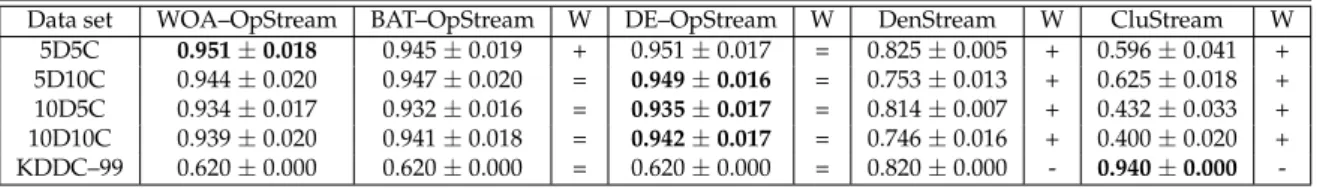
Finally, the same conclusions obtained with F-measure are drawn by interpreting the results in 423
table4, where the Rand-Index metric is used to evaluate classification performances. Indeed, all three 424
OpStream variants statistically outperform the deterministic methods. This goes to show that the 425
proposed method is performing very well regardless of the optimisation strategy, and it is always better 426
or competitive with state-of-the-art algorithms. Unlike the case in table2, the best performances in 427
terms of average value or those obtained with DE rather than WOA. However, the difference between 428
the two variants is minimal and the Wilocoxon Rank-Sum test does not detect differences between the 429
two variants. 430
Table 4. Average Rand-Index ± Standard Deviation and Wilcoxon Rank-Sum Test (reference = WOA–OpStream) for WOA–OpStream against BAT–OpStream, DE–OpStream, DenStream and CluStream on each strdata set.
Data set WOA–OpStream BAT–OpStream W DE–OpStream W DenStream W CluStream W
5D5C 0.951±0.018 0.945±0.019 + 0.951±0.017 = 0.825±0.005 + 0.596±0.041 +
5D10C 0.944±0.020 0.947±0.020 = 0.949±0.016 = 0.753±0.013 + 0.625±0.018 + 10D5C 0.934±0.017 0.932±0.016 = 0.935±0.017 = 0.814±0.007 + 0.432±0.033 + 10D10C 0.939±0.020 0.941±0.018 = 0.942±0.017 = 0.746±0.016 + 0.400±0.020 + KDDC–99 0.620±0.000 0.620±0.000 = 0.620±0.000 = 0.820±0.000 - 0.940±0.000
-Summarising, OpStream displays the best global performance, with WOA–OpStream and 431
DE–OpStream being the most preferable variants. Statistically, WOA–OpStream and DE–OpStream 432
have equivalent performances over different data sets and according to three different evaluation 433
metrics. In this light, the WOA variant is preferred as requiring the tuning of only two parameters, 434
against the three required in DE, to function optimally. 435
A final observation can be done by separating results from synthetic data sets andKDDC–99. If in 436
the first case the supremacy of OpStream is evident, a deterioration of the performances can be noted 437
when the later data set is used. In this light, one can understand that the proposed method presents 438
room for improvement of handling data streams with uneven distribution of class instances as those 439
presented inKDDC–99[53]. 440
7. Further Analyses 441
In the light of what observed in section6, the WOA algorithm is to be preferred over DE and BAT 442
to perform the optimisation phase. Hence, it is reasonable to consider the WOA–OpStream variant as 443
the default OpStream algorithm implementation. 444
This section concludes this piece of research with a thorough analysis of this variant in terms of 445
sensitivity, scalability, robustness and flexibility to handle overlapping multi-density clusters. 446
7.1. Scalability Analysis 447
A scalability analysis is performed to test how OpStream behaves, in terms of execution time 448
(seconds) needed to process 100, 000 data points per data set, over data sets having increasing 449
dimension values or increasing number of clusters. Data sets suitable for this purpose are easily 450
generated with the MOA platform, as previously done for the comparative analysis in section6. 451
This experimentation was performed in a personal computer equipped with an AMD Ryzen 5 452
2500U Quad-Core (2.0GHz) CPU Processor and 8GB RAM. Opstream was run with the following 453
parameter setting:λ=1000,e=0.1,β=4, WOA swarm size equal to 20 and maximum number of 454
allowed iterations equal to 10. 455
Execution time is plotted over increasing dimension values (for the the data points) in figure2. 456
Figure 2.Scalability to Number of Data Dimensions
(data dimension value).
Execution time is plotted over increasing number of clusters (in the the data sets) in figure3. 457
Figure 3.Scalability (number of clusters).
Regardless of the number of clusters, execution time seems to grow linearly with the 458
dimensionality of the data points, for low dimension values, to then saturate when the dimensionality 459
is high. Lower the number of clusters, later the saturation phenomenon takes place. With 5 clusters 460
this occurs at approximately 40 dimension values. In the case of 20 clusters, saturation occurs earlier at 461
approximately 25 dimension values. This is one of the strengths of the proposed method, as its time 462
complexity does not require polynomial times. 463
Conversely, no saturation takes place when execution time is measured by increasing the number 464
of clusters. Also in this case, the time complexity seems to grow linearly with the number of clusters. 465
7.2. Noise Robustness Analysis 466
The MOA platform allows for the injection of increasing noise levels into the dataset5D10Cand 467
10D5Cdata sets. 468
The five noise levels indicated in figure5and6were used and the OpStream algorithm was run 469
30 times for each one of the 10 classification problems (i.e. five noise levels×2 data sets) with the same 470
parameter setting used in section7.1. Results were collected to display average F-Measure, Purity and 471
Rand-Index relative to5D10C, i.e. table5, and10D5C, i.e. table6. 472
Table 5.Average OpStream performances over or5D10Cat multiple noise levels.
Noise Level F-Measure Purity Rand-Index
0% 0.846 0.986 0.934
3% 0.798 0.988 0.909
5% 0.808 0.983 0.892
8% 0.768 0.993 0.881
10% 0.774 0.972 0.880
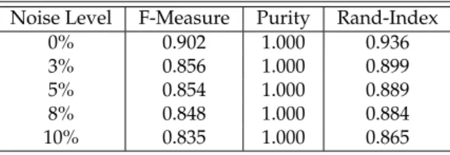
Table 6.Average OpStream performances over or10D5Cat multiple noise levels.
Noise Level F-Measure Purity Rand-Index
0% 0.902 1.000 0.936
3% 0.856 1.000 0.899
5% 0.854 1.000 0.889
8% 0.848 1.000 0.884
10% 0.835 1.000 0.865
From these results, it is clear that OpStream is able to retain approximately 95% of its original 473
performance as long as the level does not exceed the 5% level. Then, performances slightly decrease 474
OpStream seems to be robust to noise, in particular when classifying data sets with high dimensional 475
data points and a low number of clusters number. 476
7.3. Sensitivity Analysis 477
Five parameters must be tuned before using OpStream for clustering dynamic data streams. In 478
this section, the impact of each parameter on the classification performance is analysed in terms of 479
Rand-Index value. 480
To perform a thorough sensitivity analysis 481
• the sizeλof landmark time window model is examined in the range[100, 5000]∈N;
482
• theevalue for thee-neighbourhood method is examined within[0, 1]∈R;
483
• the effect of theage thresholdis examined by tuningβin the interval[1, 10]∈N;
484
• the WOA swarm sizes under analysis are obtained by adding 5 candidate solutions per 485
experiment, from an initial value of 5 candidate solutions to a maximum of 30 candidate solutions; 486
• the computational budget for the optimisation process, expressed in terms of “max iterations” 487
number, is increased by 5 iterations per experiment starting with 5 up to a maximum of 30 488
iterations. 489
OpStream was run on three data sets for this sensitivity analysis, namely5D10C,10D5CandKDDC–99, 490
and results graphically shown in the figures reported below. 491
Figure4shows that too high window sizes are not beneficial and the best performances are 492
obtained win the rage[500, 2000]data points. In particular, a peak is obtained with a size of 1000 for 493
the two artificially prepared data sets. Conversely, slightly inferior sizes might be preferred for the 494
KDDC–99data set. In general, there is no need in using more than 2000 data points are the performance 495
will remain constant or slightly deteriorate. 496
Figure 4.Sensitivity to the windows size parameterλ.
With reference to figure5, it evident thatedoes not require fine-tuning in a wide range as the best 497
performances are obtained within[0.1, 0.2]and then linearly decreases over the remaining admissible 498
values. This can be easily explained as too low values would prevent microclusters from merging 499
while too high values will force OpStream to merge dissimilar clusters. In both cases, the outcome 500
would be a very poor classification. This observation facilitates the tuning process as it means that 501
worth trying values foreare 0.1 and 0.2 and perhaps one or two intermediary values. 502
As forβ, the curves in figure6show that OpStream is not sensitive to the value chosen for 503
removing outdated clusters as long asβ≥2. This means that clusters can be technically be left in the 504
buffers for a long time without affecting the performance of the classifier. From a more practical point 505
of view, for memory issues, it is preferable to free buffers from unnecessary microclusters timely, A 506
sensible choice isβ=4, as too low values might prevent similar clusters from being merged due to the 507
lack of time required for performing such process. 508
Figure 6.Sensitivity to the AS parameterβ.
It can be noted that a small number of candidate solutions is used for the optimisation phase. This 509
choice was made for multiple reasons. First, it’s been recently shown that a high number of solutions 510
can increase structural biases of the algorithm [54], which is not wanted as the algorithm has to be 511
“general-purpose” to handle all possible scenarios obtained in the dynamic domain. Second, due to the 512
time limitations related to the nature of this application domain, a high number of candidate solutions 513
is to be avoided as it would slow down the converging process. This is not admissible in real-time 514
domain where also the computational budget is kept very low. Third, as shown in figure7the WOA 515
method used in OpStram seems to work efficiently regardless of the employed number of candidate 516
solutions, as long as it is greater than 20. 517
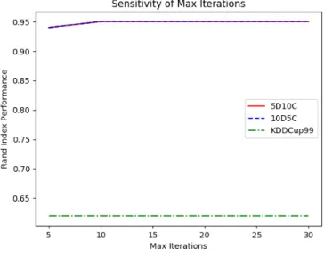
Similar conclusions can be done for the computational budget. According to figure8, it is not 518
necessary to prolong the duration of the WOA optimisation process for more than 10 iterations. 519
This makes sense in dynamic domains where the problem changes very frequently thus making the 520
exploitation phase less important. 521
Figure 8.Sensitivity tomaxIterations 7.4. Comparison with Past Studies on Intrusion Detection
522
One last comparison is performed to complete this study. This is performed on a specific application domain, i.e. network intrusion detection, by means of the “KDD–cup 99” database [55]. The comparison algorithms employed in this work, i.e. DenStream and CluStream , were both tested on this data set in their original papers [18] and [25] respectively. Despite the fact that OpStream is not meant for data sets with overlapping multi-density clusters, as in KDD–cup 99, we executed it over such data set to test its versatility. Results are displayed in table7where the last column indicates the average performance of the ckustering method by computing
AVG= F-Measure+Purity+Rand-Index
3 . (25)
Table 7.Results obtained with the KDD–cup 99 [55] data set for intrusion detection.
Algorithm F-Measure Purity Rand-Index AVG
OpStream 0.46 1.00 0.62 0.69
DenStream 0.65 1.00 0.82 0.82
ClusStream 0.14 0.42 0.94 0.50
Surprisingly, OpStream has an AVG better performance than CluStream, due to the fact that 523
significantly outperforms it in terms of F-Measure and Purity, and display a state-of-the-art behaviour 524
in terms of Purity value. As expected, DenStream provides the best performance, thus being preferable 525
in this application domain unless a fast real-time response is required. In the latter case, its high 526
computational cost could prevent DenStream from being successfully used [18]. 527
8. Conclusion and Future Work 528
Experimental numerical results show that the proposed OpStream algorithm is a promising 529
tool for clustering dynamic data streams as it is competitive and outperforms the state-of-the-art on 530
several occasions. This approach can then be applied in several challenging application domains 531
where satisfactory results are difficult to be obtained with clustering methods. Thanks to its 532
optimisation-driven initialisation phase, OpStream displays high accuracy, robustness to noise in 533
the data set and versatility. In particular, we found out that its WOA implementation is efficient, 534
scalable (both in term of data set dimensionality and number of clusters) and resilient to parameters 535
variations. Moreover, due to a low number of parameters to be tuned in WOA, this optimisation 536
algorithm is preferred over other approaches returning similar accuracy values as DE and BAT. Finally, 537
this study clearly shows that hybrid clustering methods are promising and more suitable that classic 538
approaches to address challenging scenarios. 539
Possible improvements can be done to address some of the aspects arose during the experimental 540
section. First, the deterioration of the performance over unevenly distributed data sets, asKDDC-99, 541
will be investigated. A simple solution to this problem is to embed non-density-based clustering 542
algorithms into the OpStream framework. Second, since the proposed methods do not benefit from 543
prologues optimisation processes (as shown in figure8), probably because of the dynamic nature of 544
the problem, optimisation algorithm employing “restart” mechanisms will be implemented and tested. 545
These algorithms usually work on a very short computational budget and handle dynamic domains 546
better than other by simply re-sampling the initial point where a local search routine is applied, as e.g. 547
[56], or by also adding to it information from previously past solution with the “inheritance” method 548
[57–59]. 549
It is also worthwhile to extend OpStream to handle overlapping multi-density clusters in dynamic 550
data streams, as these cases are not currently addressable and are common in some real-world scenarios, 551
such as network intrusion detection [53] and Landsat satellite image discovery [60]. 552
Author Contributions: All authors contributed to the draft of the manuscript, read and approved the final 553
manuscript. 554
Funding:This research received no external funding. 555
Conflicts of Interest:The authors declare no conflict of interest. 556
References 557
558
1. Modi, K.; Dayma, R. Review on fraud detection methods in credit card transactions. 2017 International 559
Conference on Intelligent Computing and Control (I2C2), 2017, pp. 1–5. doi:10.1109/I2C2.2017.8321781. 560
2. Moodley, R.; Chiclana, F.; Caraffini, F.; Carter, J. Application of uninorms to market basket analysis. 561
International Journal of Intelligent Systems2019,34, 39–49. doi:10.1002/int.22039. 562
3. Moodley, R.; Chiclana, F.; Caraffini, F.; Carter, J. A product-centric data mining algorithm 563
for targeted promotions. Journal of Retailing and Consumer Services 2019, p. 101940. 564
doi:https://doi.org/10.1016/j.jretconser.2019.101940. 565
4. Zarpelão, B.B.; Miani, R.S.; Kawakani, C.T.; de Alvarenga, S.C. A survey of intrusion 566
detection in Internet of Things. Journal of Network and Computer Applications 2017, 84, 25 – 37. 567
doi:https://doi.org/10.1016/j.jnca.2017.02.009. 568
5. Masud, M.M.; Chen, Q.; Khan, L.; Aggarwal, C.; Gao, J.; Han, J.; Thuraisingham, B. Addressing 569
Concept-Evolution in Concept-Drifting Data Streams. 2010 IEEE International Conference on Data 570
Mining, 2010, pp. 929–934. doi:10.1109/ICDM.2010.160. 571
6. Gharehchopogh, F.S.; Gholizadeh, H. A comprehensive survey: Whale Optimization 572
Algorithm and its applications. Swarm and Evolutionary Computation 2019, 48, 1 – 24. 573
doi:https://doi.org/10.1016/j.swevo.2019.03.004. 574
7. Hardi M. Mohammed, S.U.U.; Rashid, T.A. A Systematic and Meta-Analysis Survey of 575
Whale Optimization Algorithm. Computational Intelligence and Neuroscience 2019, 2019, 25. 576
doi:https://doi.org/10.1155/2019/8718571. 577
![Figure 1. A graphical representation of the “border microclusters” concept [36]](https://thumb-us.123doks.com/thumbv2/123dok_us/10227036.2926551/13.892.275.586.364.529/figure-graphical-representation-border-microclusters-concept.webp)