Relating the Knowledge Production Function to Total Factor Productivity: An Endogenous Growth Puzzle

(1)

IMF Staff Papers Vol. 53, No. 2

Relating the Knowledge Production Function to Total

Factor Productivity: An Endogenous Growth Puzzle

YASSER ABDIH AND FREDERICK JOUTZ*

The knowledge production function is central to research and development–based growth models. This paper empirically investigates the knowledge production function and intertemporal spillover effects using cointegration techniques. Time-series evidence suggests there are two long-run cointegrating relationships. The first captures a long-run knowledge production function; the second captures a long-run positive relationship between total factor productivity (TFP) and the knowledge stock. The results indicate that strong intertemporal knowledge spill-overs are present and that the long-run impact of the knowledge stock on TFP is small. This evidence is interpreted in light of existing theoretical and empirical evidence on endogenous growth. [JEL O4, O3, C5]

T

he most recent advancement of endogenous growth theory has been the emer-gence of research and development–based (R&D-based) models of growth in the seminal papers of Romer (1990), Grossman and Helpman (1991a and 1991b), and Aghion and Howitt (1992). This class of models aims to explain the role of technological progress in the growth process. R&D-based models view technol-ogy as the primary determinant of growth and treat it as an endogenous variable.

*Yasser Abdih is an Economist in the IMF Institute. Frederick Joutz is a Professor of Economics at The George Washington University. The authors would like to thank Ralph Chami, Robert Flood, Tim Fuerst, Arthur Goldsmith, Jim Hirabayashi, Costas Mastrogianis, Stephanie Shipp, Holger Wolf, and an anonymous referee for providing valuable comments. Yasser Abdih also thanks John Kendrick. A pre-liminary version of this research was awarded the John Kendrick Prize, which supports research in the areas of productivity and growth.

(2)

RELATING THE KNOWLEDGE PRODUCTION FUNCTION TO TFP

At the heart of R&D-based growth models is a knowledge/technology pro-duction function that describes the evolution of knowledge creation. According to that function, the rate of production of new knowledge depends on the amount of labor engaged in R&D and the existing stock of knowledge available to these researchers. A crucial debate framed by the work of Romer (1990) and Jones (1995a) (within the R&D-based growth literature) is centered on the functional form of the knowledge production function. Specifically, the debate is centered on how strongly the flow of new knowledge depends on the existing stock of knowl-edge. Intuitively, the dependence of new knowledge on the existing stock is intended to capture an “intertemporal spillover of knowledge” to future researchers—that is, knowledge or “ideas” discovered in the past may facilitate the discovery or creation of “ideas” in the present. Hence, the debate is concerned with the magnitude or the strength of these intertemporal knowledge spillovers. As we will discuss, different assumptions on the magnitude of knowledge spillovers generate completely differ-ent predictions for long-run growth.

This paper contributes to the empirical understanding of R&D-based growth models in the following ways. We use time-series data for the U.S. economy over the postwar period and directly estimate the parameters of the knowledge pro-duction function. This allows us to directly assess the magnitude of knowledge spillovers, the source of the Romer-Jones debate. To achieve this goal, we exploit historical time series of patent filings to construct knowledge flows and stocks. Hence, this paper draws on an extensive body of work that uses patents as mea-sures of innovative output and regards them as useful statistics for measuring eco-nomically valuable knowledge—for example, Hausman, Hall, and Griliches (1984); Griliches (1989 and 1990); Joutz and Gardner (1996); and Kortum (1997). We employ Johansen’s (1988 and 1991) maximum-likelihood cointegration pro-cedure to estimate the U.S. knowledge production function. Cointegration tech-niques are needed because, like most macroeconomic time series, the inputs and output of the knowledge production function can be plausibly characterized as nonstationary and integrated of order one, or I(1) time series. Hence, if estimated using conventional methods like ordinary least squares (OLS), the knowledge production function will suffer from spurious correlations. Johansen’s cointegra-tion procedure corrects for any spurious correlacointegra-tions that may exist in the data and explicitly accounts for the potential endogeneity of the inputs of the knowl-edge production function.

In his seminal paper, Romer (1990) assumes a knowledge production function in which new knowledge is linear in the existing stock of knowledge, holding the amount of research labor constant. The implication of this strong form of knowl-edge spillovers is that the growth rate of the stock of knowlknowl-edge is proportional to the amount of labor engaged in R&D. Hence, policies—such as subsidies to R&D—that increase the amount of labor allocated to research will increase the growth rate of the stock of knowledge. Because the Romer model is one in which long-run per capita growth is driven by technological progress/knowledge growth, such policies will increase long-run per capita growth in the economy.

In an influential paper, Jones (1995b) questions the empirical validity of the Romer model. The Romer model predicts that an increase in the amount of research

(3)

Yasser Abdih and Frederick Joutz

labor should increase the growth rate of the stock of knowledge, a prediction that depends critically on strong positive spillovers in knowledge production. Jones tests the validity of this prediction by appealing to data on total factor productivity (TFP) growth (as a proxy for knowledge growth) and R&D scientists and engineers (as a proxy for research labor). He argues that, in the United States, the number of R&D scientists and engineers has increased sharply over the postwar period, while TFP growth has been characterized by relative constancy at best. This weak rela-tionship between the number of R&D scientists and engineers and TFP growth led Jones to conclude that the magnitude of knowledge spillovers assumed by Romer is too large. To be consistent with the empirical evidence, Jones argues that a smaller magnitude of knowledge spillovers needs to be imposed. Imposing a smaller magnitude of knowledge spillovers, however, alters the key implication of Romer’s model. Specifically, in the modified model developed by Jones (1995a), long-run growth depends only on exogenously given parameters and, hence, is invariant to policy changes such as subsidies to R&D.

We study the cointegration properties of data on new knowledge (measured by the flow of new patents), the existing knowledge stock (measured by the patent stock), R&D scientists and engineers, and TFP. We include TFP in the empirical model for three reasons. First, Jones (1995b) uses TFP as a measure of knowledge, whereas we use the patent stock. The inclusion of TFP in the empirical model allows us to capture how closely our patent measure relates to Jones’s measure. Second, long-run economic growth depends on TFP, which is the application and embodiment of knowledge. Third, it enables the estimated empirical model to shed some light on the observed weak relationship between TFP growth and the number of R&D scientists and engineers.

The paper finds two long-run cointegrating relationships. The first captures a long-run knowledge production function in which the flow of new knowledge depends positively on the existing stock of knowledge and the number of R&D sci-entists and engineers. The second captures a long-run positive relationship between TFP and the stock of knowledge (patents). The results indicate the presence of strong intertemporal knowledge spillovers, which is consistent with the Romer (1990) model. The long-run elasticity of new knowledge creation, with respect to the existing stock, is at least as large as unity. However, the long-run impact of the knowledge (patent) stock on TFP is small: Doubling the stock of knowledge (patents) is estimated to increase TFP by only 10 percent in the long run. In other words, the results suggest that although R&D scientists and engineers greatly ben-efit from the knowledge and ideas discovered by prior research, the knowledge they produce seems to have only a modest impact on measured TFP.

These results seem to suggest a new interpretation of the empirical evidence documented by Jones (1995b). The observed weak relationship between the num-ber of R&D scientists and engineers and TFP growth found by Jones is not neces-sarily an indication of weak intertemporal knowledge spillovers. We feel that knowledge—the output from researchers’ effort—is an important intermediate step to TFP. This paper provides some evidence that the rate of diffusion of new knowl-edge into the productive sector of the U.S. economy has been slow over the past 20 years. The application and embodiment of knowledge into productivity is

(4)

com-RELATING THE KNOWLEDGE PRODUCTION FUNCTION TO TFP

plex and the diffusion is slow. Our empirical work contributes to understanding and reconciling some of the spillover effects and issues raised by Jones (1995b).

The rest of the paper is organized as follows. Section I presents a simple R&D-based growth model with the focus on the Romer-Jones debate and the knowledge production function. Section II describes the data on the inputs and output of that function. Section III looks at the univariate and multivariate time-series properties of the data and estimates the knowledge production function. Section IV discusses the main results of the paper and their interpretation. Finally, Section V offers some concluding remarks.

I. The Romer-Jones Debate on Knowledge Production

In this section, we present a simplified version of the R&D-based growth models of Romer (1990) and Jones (1995a). We focus on the basic elements and the key macroeconomic implications for long-run growth. As such, we present the model in “reduced form” and, in doing so, suppress the microfoundation and market structure components. This is done purely for ease of exposition.

A Simple R&D-Based Growth Model

The model has four variables: output (Y), capital (K), labor (L), and technology or knowledge (A).1_{There are two sectors: a goods sector that produces output, and an} R&D sector that produces new knowledge. Labor can be freely allocated to either of the two sectors, to produce output (LY) or to produce new knowledge (LA). Hence, the economy is subject to the following resource constraint:LY+LA=L.

Specifically, output is produced according to the following Cobb-Douglas pro-duction function with labor augmenting (Harrod-neutral) technological progress:

New knowledge or new ideas are generated in the R&D sector. Let Adenote the stock of knowledge/technology available in the economy. The knowledge stock can be thought of as the accumulation of all ideas that have been invented or developed. Then,A.represents the flow of new knowledge or the number of new ideas generated in the economy at a given point in time. New ideas are produced by researchers,LA, according to the following production function:

where δ–denotes (average) research productivity, that is, the number of new ideas generated per researcher. In turn –δis modeled as a function of the existing stock of knowledge/ideas (A) and the number of researchers (LA) according to the following:

δ δ₌ φ λ− δ_> , , ( ) A L_A1 ₀ ₃ A.= δ L_A, ( )2 Y =Kα(ALY)−α < <α 1 0 1 1 ,where . ( )

(5)

where δ,φ, and λare constant parameters. The presence of the term Aφin equa-tion (3) is intended to capture the dependence of current research productivity on the stock of ideas already discovered. Ideas formulated in the past may facilitate the discovery or creation of ideas in the present, in which case current research productivity is increasing in the stock of knowledge (φ> 0). Hence,φ> 0 captures a positive “spillover of knowledge” to future researchers and is referred to as the “standing-on-shoulders” effect. Alternatively, it is possible that the most obvious ideas are discovered first and new ideas become increasingly harder to find over time. In this case, current research productivity is decreasing in the stock of ideas already discovered. This corresponds to φ< 0, the “fishing-out” effect.2

The presence of the term Lλ−1

A in equation (3) captures the dependence of research productivity on the number of people seeking new ideas at a given point in time. For example, it is quite possible that the greater the number of people searching for ideas, the more likely it is that duplication or overlap in research would occur. In that case, if we double the number of researchers (LA), we may less than double the number of unique ideas or discoveries ( A.). This notion of dupli-cation in research, or the “stepping-on-toes” effect, can be captured mathematically by allowing for 0 < λ< 1, in which case research productivity is decreasing in LA. Taken together, equations (2) and (3) suggest the following knowledge pro-duction function:

That is, the number of new ideas or new knowledge at any given point in time depends on the number of researchers and the existing stock of ideas.

Growth Implications of the Model

Given the above setup, it can be easily shown that a balanced growth path/steady state exists for this economy, which is defined as a situation in which all variables grow at constant (possibly zero) rates. Along this path, output per worker (y) and the capital-labor ratio (k) grow at the same rate as technology (A):

where gy, gk, and gArespectively denote the steady state growth rate of y, k,and A. Hence, R&D-based growth models share the prediction of the neoclassical Solow model that technological progress is the source of sustained per capita growth. If technological progress ceases, so will long-run per capita growth. Therefore, to solve for the steady state per capita growth rate in this economy, it suffices to solve for gA, which is in turn determined by the knowledge production function as shown below. We focus on two versions of that function: Romer (1990) and Jones (1995a). Their versions have completely different implications for long-run growth.

g_y=g_k =g_A, ( )5 A L A A . . ( ) = δ λ φ 4

2_{The case in which}_{φ =}_{0 allows the fishing-out effect to completely offset the standing-on-shoulders} effect. That is, current research productivity is independent of the stock of knowledge.

(6)

Those implications depend critically on the magnitude of the knowledge spillover parameter assumed (φin equation (4)).

Romer’s Model

Romer (1990) assumes a particular form of the knowledge production function in equation (4). He imposes the restrictions φ =1 and λ =1. The key restriction made by Romer, however, is φ =1. This makes A.linear in A,and generates growth in the stock of knowledge (A./A) that depends on LAunit homogeneously:

Equation (6) pins down the steady state growth rate of the stock of knowledge, gA, as

That is, the steady state growth rate of the stock of knowledge and per capita out-put by equation (5) depend positively on the amount of labor devoted to R&D. This key result has important policy implications: Policies that permanently increase the amount of labor devoted to R&D—a subsidy that encourages research, for example—have a permanent long-run effect on the growth rate of the economy. This “growth effects” result is a hallmark of the Romer (1990) model and many existing R&D-based endogenous growth models, including the important contri-butions of Grossman and Helpman (1991a and 1991b) and Aghion and Howitt (1992). This result stands in sharp contrast to the neoclassical Solow model, in which changes in variables that are potentially affected by policy have short- and medium-run effects but no long-run growth effects.

Jones’s Critique

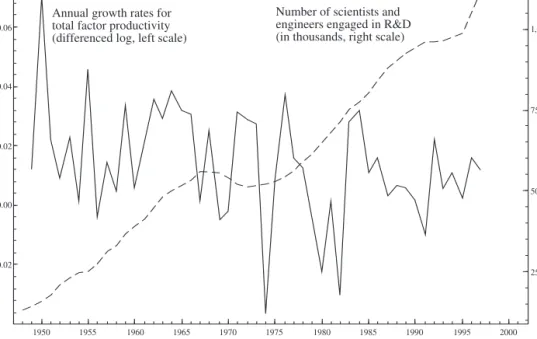
Equation (7) predicts “scale effects”: An increase in the level of resources devoted to R&D—as measured by LA—leads to an increase in the growth rate of the econ-omy. In an influential paper, Jones (1995b) presents time-series evidence against scale effects using one measure for LAand one for A./Afor the United States over the postwar period. He represents LA by the number of scientists and engineers engaged in R&D. This is perfectly reasonable because, theoretically,LA captures the R&D workforce. Jones uses TFP growth as a proxy for A./A,which is shown in Figure 1 for the U.S. economy. TFP growth appears to fluctuate around a rela-tively constant mean of about 1.4 percent per year over the postwar period. Therefore, LA should, like A./A, be relatively constant and exhibit no persistent increase. Otherwise, Romer’s knowledge production function and the resulting scale effects are inconsistent with the time-series evidence.

Figure 1 also plots LA, as measured by the number of scientists and engineers engaged in R&D for the U.S. economy. As Figure 1 reveals,LAis not relatively

g_A= δL_A. ( )7 A A LA . . ( ) = δ 6

(7)

constant over the postwar period. Rather, it exhibits a strong upward trend, rising from about 100,000 in 1950 to about 1 million by 1997. Therefore, the knowledge production function in equation (6), which lies at the heart of the Romer (1990) model, is inconsistent with the time-series data.3

Jones’s Alternative

Because the rejection of the scale effects prediction is rooted in the incongruence of the knowledge production function with the time-series data, it seemed sensi-ble for Jones to tackle and modify its functional form to develop an alternative specification that is consistent with the observed time-series pattern of the data. Jones (1995a) actually shows that relaxing the assumption φ =1 generates a steady state that is consistent with the rising number of research workers observed in the data. To do that, consider once again the knowledge production function in equa-tion (4) and divide both sides of that equaequa-tion by A:

A A L A A . . ( ) =δ ₋ λ φ 1 8

3_{The criticism by Jones (1995b) is not exclusive to the Romer (1990) model, but rather it is a criticism} against many existing R&D-based endogenous growth models that share Romer’s knowledge production function. – 0.02 0.00 0.02 0.04 0.06 1950 1955 1960 1965 1970 1975 1980 1985 1990 1995 2000 250 500 750 1,000 Annual growth rates for

total factor productivity (differenced log, left scale)

Number of scientists and engineers engaged in R&D (in thousands, right scale)

Sources: National Science Foundation, Science and Engineering Indicators–2000; Jones (2002); Machlup (1962); and Bureau of Labor Statistics.

Figure 1. Total Factor Productivity Growth and Research and Development (R&D) Scientists and Engineers in the United States

(8)

In the steady state, the growth rate of Ais constant by definition. Therefore, the right-hand side of equation (8) must be constant in the steady state, which means that Lλ_Aand A1−φ_{must grow at the same rate. That is,}

Now λis a positive parameter and A./Ais always positive and constant in the steady state. Therefore, equation (9) implies that a constant steady state growth of Awill be consistent with a rising LA, that is,L.A/LA> 0, provided that φis less than unity. Hence, Jones (1995a) argues that assuming φ< 1 is consistent with the observed relative constancy of TFP growth (the proxy of A./A used by Jones) in spite of the rising trend of R&D scientists and engineers. Moreover, with φ< 1 imposed, the scale effects of the Romer (1990) model are removed. This can be seen formally by solving for the steady state growth rate of Afrom equation (9) as follows:

That is, the long-run growth rateof the stock of knowledge, which is also the long-run growth rate of per capita output by equation (5), depends on the growth rate of LA rather than its level. Note that positive knowledge spillovers are not ruled out. The parameter capturing knowledge spillovers,φ, may plausibly be pos-itive and large. What the above discussion does suggest is that the degree of posi-tive knowledge spillovers assumed by Romer is arbitrary and inconsistent with the time-series evidence. A weaker magnitude of such spillovers is needed to achieve congruency with the evidence.

Now, along the balanced growth path/steady state, the growth in the number of research workers will be equal to the growth rate of the labor force/population. If it were greater, then the number of researchers would eventually exceed the labor force, which is not feasible. Let n denote the growth rate of the labor force/population, which Jones (1995a), following the literature, assumes to be exogenously given. Then, in the steady state,L.A/LA= L

.

/L= n. Substituting this relationship into equation (10) yields the following:

Equation (11) implies that long-run growth depends on φ,λ, and n,parameters that usually are assumed to be exogenously given. Hence, long-run growth in the Jones (1995a) model is independent of policy changes such as subsidies to R&D. Because the returns to knowledge accumulation are assumed to be less than unity (φ< 1), such changes will affect the growth of Aalong the transition path to a new steady state, and these “transitional growth effects” will be translated into long-run level effects. Simply stated, subsidies to R&D will alter the long-run level of the

gA= ₋ n λ φ 1 . ( )11 g L L A A A = − λ φ 1 10 . . ( ) λL φ L A A A A . . . ( ) = −

(

1

)

9

(9)

stock of knowledge but not its long-run growth rate. In Jones’s (1995a) modified model, long-run growth is invariant to policy.

II. Data

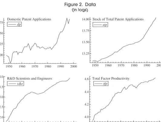
In this section, we describe the variables used to empirically reconsider the theo-retical relationships between the knowledge production function and productivity. The four variables include patent applications, the stock of patents, the number of scientists and engineers engaged in R&D, and TFP. The sample frequency is annual and is available from 1948 to 1997. Variables in levels will be transformed into natural logarithms and are shown in Figure 2. Details on the construction and sources of the data are found in the appendix.

Patent applications serve as a valuable resource for measuring innovative activ-ity and have been extensively used in the patent literature as measures of techno-logical change (see, for example, Hausman, Hall, and Griliches, 1984; Griliches, Pakes, and Hall, 1987; and Kortum, 1997). Also, Griliches (1989 and 1990) argues that the aggregate count of patents can serve as a measure of shifts in technology. Joutz and Gardner (1996) argue that patent application trends are a good approxi-mation for technological output over the long run. Firms have invested resources to

1950 1960 1970 1980 1990 2000

11.00 11.25 11.50

11.75 Domestic Patent Applications_dp

1950 1960 1970 1980 1990 2000

13.25 13.50 13.75

14.00 Stock of Total Patent Applications

stp 1950 1960 1970 1980 1990 2000 12.0 12.5 13.0 13.5

14.0 _{R&D Scientists and Engineers}

s&e

1950 1960 1970 1980 1990 2000

4.0 4.2 4.4

4.6 Total Factor Productivity tfp

Sources: National Science Foundation, Science and Engineering Indicators–2000; Jones (2002); Machlup (1962); Bureau of Labor Statistics, and U.S. Patent and Trademark Office.

Figure 2. Data

(10)

develop new technologies, which they feel have economic value and for which they are willing to submit applications to capture rents from their initial investments. This paper follows the patent literature and uses patent applications to construct knowledge flows and stocks.4_{The output of the knowledge production function} should reflect new knowledge created by U.S. researchers. As such, we use domes-tic patent applications (DP) filed at the U.S. Patent and Trademark Office (USPTO) to measure new knowledge.

Figure 2 plots the log of domestic patent applications (dp). There is an overall upward trend in the series, with domestic patent applications growing at an average annual rate of 1.7 percent between 1948 and 1997. The behavior of the series since the mid-1980s is particularly striking: Since about 1985, domestic patent applica-tions have increased dramatically at an average annual rate of 5.1 percent. Jaffe and Lerner (2004) claim that much of this increase in patent applications may be spurious and does not necessarily reflect a true increase in the flow of new knowl-edge. They argue that regulatory and institutional changes simply made it easier to get a patent on unoriginal ideas, and this encouraged the filing of dubious patent applications.5

However, there is sizable evidence that much of the increase in patent appli-cations since the early 1980s has notbeen due to institutional and regulatory changes that made it easier to patent ideas that dubiously constitute an innovation, but rather the increase reflects a true surge in discovery and innovation. First, Greenwood and Yorukoglu (1997) document that the 1980s and 1990s witnessed an explosion of formation of new firms and innovation in the high-tech industries,

4_{Note that we measure knowledge/technology using patent applications rather than patent grants. The} lag between application and grants could be quite long, and it varies over time partly because of changes in the availability of resources to the U.S. Patent and Trademark Office. This notion is best articulated by Griliches (1990, p. 1690): “A change in the resources of the patent office or in its efficiency will introduce changes in the lag structure of grants behind applications, and may produce a rather misleading picture of the underlying trends. In particular, the decline in the number of patents granted in the 1970s is almost entirely an artifact, induced by fluctuations in the U.S. Patent Office, culminating in the sharp dip in 1979 due to the absence of budget for printing the approved patents.” This paper views patent applications as a much better measure of knowledge and technology than patent grants. Also, it is widely believed that patent application data are a better measure of new knowledge produced in an economy than R&D expenditures (see, for example, Joutz and Gardner, 1996). R&D expenditures are more properly thought of as inputs to technological change, whereas patents are an output. Hence, patent applications more closely approximate the output of the knowledge production function in R&D-based growth models than R&D expenditures.

5_{Specifically, in 1982, Congress established the Court of Appeals of the Federal Circuit (CAFC), a} specialized and centralized appellate court to hear patent cases. (Before 1982, patent appeals cases were heard before various district courts, which differed considerably in their interpretation of the patent law.) Jaffe and Lerner (2004, p. 2) argue that the court “has interpreted patent law to make it easier to get patents, easier to enforce patents against others, easier to get large financial awards from such enforcement, and harder for those accused of infringing patents to challenge the patents’ validity.” Moreover, the court’s rul-ings regarding the standard of “novelty” and “nonobviousness” may have made it easier for applicants to file and get a patent of dubious validity. In addition, in the early 1990s, Congress changed the patent office from an agency funded by taxpayer money to a self-financed agency, that is, one that relied exclusively on patent application fees to conduct its business. Jaffe and Lerner argue that that might have created a strong incentive for the patent officer to process applications more quickly and at minimum cost. This might have reduced the rigor by which the standards of novelty and nonobviousness are exercised when reviewing patent applications. This, in turn, encouraged the filing of dubious patent applications.

(11)

particularly in the information technology, biotechnology, and software industries. Hence, the sharp increase in patenting may indicate a “technological revolution” as emphasized by those authors. Second, it is quite possible that the use of infor-mation technology in the discovery of new ideas might have substantially boosted research productivity. Arora and Gambardella (1994) argue that this was an impor-tant source of accelerating technological change. A third possibility, emphasized by Kortum and Lerner (1998), is that the sharp increase in patenting since the mid-1980s indicates an increase in innovation driven by improvements in the management of R&D. In particular, there has been a reallocation of resources from basic research toward more applied activities and hence a resulting surge in patentable discoveries. As Kortum and Lerner (1998, p. 287) point out, “Firms are restructuring, redirecting and resizing their research organizations as part of a corporate-wide emphasis on the timely and profitable commercialization of inventions combined with the rapid and continuing improvement of technologies in use.”

In addition, several studies have argued that (the inverse of) the relative price of capital is a good indicator of the quantity of economically useful knowledge— for example, Krusell (1998) and Cummins and Violante (2002).6_{Samaniego (2005)} compares (the inverse of) the relative price of capital with patent applications for the U.S. economy over the postwar period and finds that the two series are highly positively correlated, which is supportive of the use of patent applications as a mea-sure of knowledge. More important, he observes that the growth in both series accelerated starting in the 1980s. This is consistent with the argument that the surge in patenting that started in the 1980s is not spurious but rather reflects an actual increase in the rate of innovation in the U.S. economy.

The stock of knowledge is derived from the cumulated number of total patents applied for by U.S. and foreign inventors. Patent filings are converted into a stock measure (STP) using the perpetual inventory method with a depreciation rate of 15 percent. This is typical in the U.S. patent literature (for example, Griliches (1989) and Joutz and Gardner (1996)). While this approach is ad hoc and not nec-essarily justified by theory, researchers have typically checked the robustness of their results against changes in the depreciation rate. We experimented with con-structing stocks using 0, 5, and 10 percent depreciation rates and found that the pre-cise rate made little difference. Hence, the results presented in this paper are not sensitive to changes in the depreciation rate on the stock.

As shown in Figure 2, the log of the stock of total patent applications (stp) fol-lows a strong upward trend, with the stock growing at an average annual rate of 1.9 percent between 1948 and 1997. There appears to be a substantially stronger trend since the mid-1980s, capturing the more rapid increase in (the number of) domestic patent applications that occurred over that period.

Figure 2 also plots the log of the total number of scientists and engineers engaged in R&D activities (s&e) in the United States, as compiled by the National

6_{However, although the relative price of capital has merit insofar as it captures embodied knowledge} in the capital stock, it does not capture the sources of new knowledge, which are not in physical capital.

(12)

Science Foundation. This measure was used by Jones (2002) and represents sci-entists and engineers employed in industry, the federal government, educational institutions, and nonprofit organizations. It is accepted as the best proxy for the primary input or effort in the knowledge production process. The series exhibits a very strong upward trend over the past 50 years, with the number of R&D sci-entists and engineers growing at an average annual rate of 4.3 percent over the period 1948–97.7

Finally, Figure 2 shows the plot for the log of total factor productivity (tfp), as compiled by the Bureau of Labor Statistics. TFP follows an upward trend over the postwar era, growing at an average annual rate of about 1.4 percent between 1948 and 1997. Growth appears to have slowed since 1973—the well-known produc-tivity slowdown. Before 1973, the average annual growth rate of TFP was 2.1 per-cent. After 1973, the average annual growth rate declined to about 0.7 perper-cent.

III. Estimation of Knowledge Production Functions

We employ the general-to-specific modeling approach advocated by Hendry (1986). This approach attempts to characterize the properties of the sample data in simple parametric relationships that remain reasonably constant over time and are interpretable in an economic sense. Rather than using econometrics to illustrate theory, the goal is to “discover” which alternative theoretical views are tenable and test them scientifically. The approach begins with a general hypothesis about the relevant explanatory variables and dynamic process (that is, the lag structure of the model). The general hypothesis should be considered acceptable to all adversaries. Then the model is narrowed down by testing for simplifications or restrictions on the general model.

The four macroeconomic and innovation variables are linked through two main relationships. The long-run knowledge production function and the long-run relationship between TFP and the stock of total patents (knowledge) can be spec-ified as follows:

where lowercase letters denote variables in natural logarithms. That is, dp denotes the log of the number of domestic patent applications,stpdenotes the log of the stock of total patent applications, and s&edenotes the log of the num-ber of scientists and engineers engaged in R&D. According to the above pro-duction function, U.S. R&D scientists and engineers produce U.S. patents, but

tfp=G stp( ), (13)

dp=F stp s

(

, &e

)

(12)

7_{In the late 1960s through the early 1970s, however, employment of R&D scientists and engineers} seems to have declined. The National Science Foundation (1998) documents that this is probably due to the substantial decline in federal funding for space-related R&D in the late 1960s and early 1970s after the thrust of funding in the early to mid-1960s, during which time the United States invested substantial resources in the “space race” with the Soviet Union.

(13)

they draw upon the “world” stock of knowledge.8 _{Also, the function}_F(.₎ _is assumed to be linear.9

Since Jones (1995b) used TFP as a measure of knowledge, we also include the relation G(.) for the log of TFP (tfp) in the model. This allows us to capture how closely our patent measure and Jones’s measure are related and allows us to inter-pret the results in terms of Jones’s time-series evidence on TFP and R&D sci-entists and engineers. We look at the transmission mechanism by separating the R&D effort and output. The total stock of patents represents the cumulative R&D output, which leads to higher productivity. This is consistent with the sub-stantial microproductivity literature (Jaffe, Trajtenberg, and Henderson, 1993; and Thompson and Fox-Kean, 2005) that postulates a positive dependence of TFP on the stock of patents.

The first step in the modeling approach examines the time-series properties of the individual data series. We look at patterns and trends in the data and test for stationarity and the order of integration. Second, we form a vector auto regression (VAR) system. This step involves testing for the appropriate lag-length of the sys-tem, including residual diagnostic tests and tests for model/system stability. Third, we test the system for potential cointegration relationship(s). Data series integrated of the same order may be combined to form economically meaningful series that are integrated of lower order. Fourth, we interpret the cointegrating relations and test for weak exogeneity. Based on these results, a conditional error correction model of the endogenous variables may be specified, further reduction tests are per-formed, and economic hypotheses are tested. This last step will not be perper-formed, because the primary goal is to understand the long-run relationships.

Integration Analysis

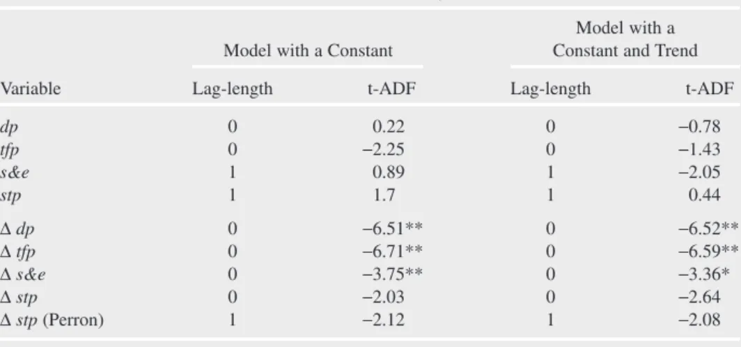
Figure 2 shows significant trends in the series and the autocorrelations were quite strong and persistent. Nelson and Plosser (1982) found that many macroeconomic and aggregate level series are shown to be well modeled as stochastic trends, that is, integrated of order one, or I(1). Simple first differencing of the data will remove the nonstationarity problem, but with a loss of generality regarding the long-run “equilibrium” relationships among the variables. We performed the standard aug-mented Dickey-Fuller (ADF) test in both levels and differences with a constant and trend. Table 1 contains the results in five columns and is divided in two. The top half is for the tests in levels and the bottom half is for the tests in first dif-ferences or whether the series in levels are I(1) and I(2), respectively. The first column lists the variables. The Akaike information criterion was used to set the

8_{In section IV, we use the stock of domestic patents as an alternative measure of the stock of} knowl-edge. We compare the results from using such a measure with the results in which the stock of total (domestic and foreign) patents is used.

9_{Recall that the R&D-based growth models of Romer (1990) and Jones (1995a) assume a} Cobb-Douglas specification for the knowledge production function expressed in terms of the levels of the vari-ables. Because the function F(.)in the text is expressed in terms of the log levels of the variables, it is assumed to be linear.

(14)

appropriate lag-length for the dependent variable in each test, which is provided in the second and fourth columns. The t-ADF statistics are reported in the third and fifth columns.

We cannot reject the null hypothesis of a unit root for all four variables in lev-els. Domestic patents, TFP, and R&D scientists and engineers reject the null of a unit root in first differences, while the stock of patents does not. However, a recur-sive analysis of the coefficient estimate and the t-ADF suggest that it is nonconstant with a break right where one might expect it: 1985. In our preliminary look at the data, we saw the acceleration in the propensity to patent and its impact on the stock of patents. We have also inspected the plot of the first difference in the logarithm of the patent stock measure and observed that there appears to be a permanent shift in the mean starting in the mid-1980s. The Perron (1989) structural break procedure was used to test whether there was a mean shift in the first difference process that caused the I(1) findings. We could not reject the (null) hypothesis of stationarity in the first difference process after correcting for the (structural) mean shift. We

con-Table 1. Augmented Dickey-Fuller (ADF) Test Results for Levels and Differences, 1953–97

Model with a

Model with a Constant Constant and Trend

Variable Lag-length t-ADF Lag-length t-ADF

dp 0 0.22 0 −0.78 tfp 0 −2.25 0 −1.43 s&e 1 0.89 1 −2.05 stp 1 1.7 1 0.44 ∆dp 0 −6.51** 0 −6.52** ∆tfp 0 −6.71** 0 −6.59** ∆s&e 0 −3.75** 0 −3.36* ∆stp 0 −2.03 0 −2.64 ∆stp(Perron) 1 −2.12 1 −2.08 Notes:

For a given variable x,the augmented Dickey-Fuller equation with a constant term included has

the following form: where εtis a white noise disturbance. The

augmented Dickey-Fuller equation with a constant and trend included adds a trend term as a right-hand-side variable to the above specification. For a given variable and specification, the table reports the number of lags on the dependent variable,p,chosen using the Akaike information criterion, and the augmented Dickey-Fuller statistic, t-ADF, which is the t-ratio on π. The statistic tests the null hypothesis of a unit root in x,i.e.,π =0, against the alternative of stationarity. Critical values at the 5 percent and 1 percent significance levels, respectively, are −2.927 and −3.581.

The symbols * and ** denote rejection of the null hypothesis at the 5 percent and 1 percent crit-ical values, respectively.

The Perron adjusted results report the test for stationarity with a structural shift in the mean with the break point at 1985, approximately 80 percent from the starting observation. The critical values tabulated by Perron (1989) are −3.82 and −4.38 at the 5 percent and 1 percent significance levels, respectively. ∆xt xt i∆xt i a i p t = − + − + + =

∑

π 1 θ ε 1 ,

(15)

clude that all of our variables are I(1) in levels, or equivalently stationary in first differences.

Cointegration Analysis

Our analysis of the inputs and output of knowledge production suggests that the processes are nonstationary. This has implications with respect to the appropriate statistical methodology. Although focusing on changes in knowledge production eliminates the problem of spurious regressions, it also results in a potential loss of information on the long-run interaction of variables (for example, Davidson and others, 1978). We examine the hypothesis of whether there exist economically meaningful linear combinations of the I(1) series: (domestic) patent filings, the stock of patents, R&D scientists and engineers, and TFP that are stationary or I(0). The Johansen (1988 and 1991) maximum likelihood procedure is used for the analysis. The procedure begins with specifying a VAR system,

where

Ytis (4 ×1) and the πis are (4 ×4) matrices of coefficients on lags of Yt. Dtis a vector of deterministic variables that can contain a linear trend, dummy-type vari-ables, or other regressors considered to be fixed and nonstochastic. Finally,etis a (4 ×1) vector of independent and identically distributed errors assumed to be nor-mal with zero mean and covariance matrix Ω—that is,et∼i.i.d. N(0,Ω). As such, the VAR is composed of a system of four equations, in which the right-hand side of each equation includes a common set of lagged and deterministic regressors.

The VAR includes our four series: the log of domestic patent applications,dp; the log of TFP,tfp;the log of the (lagged) stock of total patent applications,stpl1;10 and the log of the number of R&D scientists and engineers,s&e. The VAR also includes a constant, a trend term, and three dummy variables. The first dummy vari-able is Stepdum86, which takes the value of one after 1985 and zero otherwise. The inclusion of this variable is intended to capture the dramatic increase in patenting since the mid-1980s as discussed in detail above. The second dummy variable is Impulse9495, which takes the value of one in 1994 and 1995 and zero otherwise, and the third is Impulse96, which is zero except for unity in 1996. Impulse9495

Y Patent Filings Patent Stock R D Scientis t t t = & tts Engineers Total Factor oductivity

t t & Pr               ( ) = ,e IN , ,and D Stepdum tt t ; 0 86 Ω Immpulse Impulse 9495 96 t t t Trend               . Yt iY D e i p t i t t = + + + = −

∑

π0 π 1 14 Ψ , ( )

10_{The variable}_stpl_{1 is simply}_stp_{lagged one period. Because}_stp_{is calculated as end of period stocks,} we enter it with a lag in the VAR and cointegration analysis.

(16)

captures several institutional changes in the U.S. patent policy: the movement toward the typical international patent system policy of granting 20-year awards instead of 17-year awards, and the fact that 12-year patent renewal fees were col-lected for the first time in the United States in 1994–95 (Kortum, 1997). Impulse96 captures the instantaneous negative response by agents facing an increased cost of patent applications (see Figure 2).11

Following Johansen and Juselius (1990), the VAR model provides the basis for cointegration analysis. Adding and subtracting various lags of Yyields an expres-sion for the VAR in first differences. That is,

where

If π is a zero matrix, then modeling in first differences is appropriate. The matrix πmay be of full rank or less than full rank, but of rank greater than zero. When rank(π) =4,then the original series are not I(1), but in fact I(0); modeling in differences is unnecessary. But, if 0 < rank(π) ≡r< 4,then the matrix πcan be expressed as the outer product of two full column rank (4 × r) matrices αand β where π = αβ′. This implies that there are 4 −runit roots in πY.The VAR model can then be expressed in error correction form. That is,

The matrix β′ contains the cointegrating vector(s) and the matrix α has the weighting elements for the rth cointegrating relation in each equation of the VAR. The matrix rows of β′Yt−1are normalized on the variable(s) of interest in the coin-tegrating relation(s) and interpreted as the deviation(s) from the long-run equilib-rium condition(s). In this context, the columns of αrepresent the speed of adjustment coefficients from the long-run or equilibrium deviation in each equation. If the coefficient is zero in a particular equation, that variable is considered to be weakly exogenous and the VAR can be conditioned on that variable.

Unrestricted Model and Testing for Cointegration

Before conducting the cointegration tests, the appropriate lag-length for the VAR must be determined and a constant model found. The lag-length is not known a priori, so some testing of lag order must be done to ensure that the estimated resid-uals of the VAR are white noise—that is, they do not suffer from autocorrelation,

∆Yt Yt Γ ∆i Y ΨD e i p t i t t = + ′ − + + + = − −

∑

π0 αβ 1 1 1 16 . ( ) Γi= −

(

πi+1+ . . . +πp

)

, i=1, . . . ,p−1 and π≡ πii i p I =

∑

  1  − . ∆Yt Yt Γ ∆i Y ΨD e i p t i t t = + − + + + = − −

∑

π0 π 1 1 1 15 , ( )

11_{Statistically, the inclusion of}_Impulse_9495,_Impulse_{96, and}_Stepdum_{86 in the VAR results in a} sub-stantial improvement in the fit of the model and much better residual diagnostics, and ensures a statisti-cally stable/constant VAR.

(17)

non-normality, and so on. We started with a VAR that includes four lags on each variable, denoted VAR(4), then we estimated a VAR with three lags, VAR(3), and tested whether the simplification from VAR(4) to VAR(3) was statistically valid. The process was repeated sequentially down to a VAR with a single lag, VAR(1). Based on sequential F-tests for model reduction, we concluded that the simplifi-cation to a VAR with one lag is statistically valid. This result is also supported by the Schwarz criterion and the Hannan-Quinn criterion, which were minimized when the VAR had a single lag. Moreover, the VAR with a single lag produced residuals that are serially uncorrelated, normal, and homoskedastic. We have also estimated VAR(1) recursively to test for model constancy. The recursively esti-mated chow tests indicated that VAR(1) is statistically stable. Hence, we proceed with the analysis using the VAR(1) model. For a more detailed discussion on model reduction, residual diagnostics, and model stability results, please refer to the working paper version of this paper (Abdih and Joutz, 2005).

The cointegration analysis proceeds in several steps: testing for the existence of cointegration, interpreting and identifying the relationship(s), and conducting inference tests on the coefficients from theory and weak exogeneity. Testing per-mits reduction of the unrestricted general model to a final restricted model with-out loss of information.

Table 2 presents the initial test for cointegration and is divided into three pan-els. Panel A contains results on the possible number of cointegrating relations. There are four columns for the eigen-values, null hypothesis, Trace statistic, and its associated p-value. In the first row, the null hypothesis (r =0) is that there are zero cointegrating vectors, as opposed to the alternative that there are more than zero cointegrating vectors. This hypothesis is soundly rejected with a trace statistic of 184.03 and no measurable p-value. When the possible maximum number of cointegrating relations is one against the alternative hypothesis that there is more than one, the test statistic is 58.87 and the p-value is [0.00]. This suggests that there are at least two cointegrating vectors. We cannot reject the null hypothesis that there are at most two cointegrating relations in the third row.

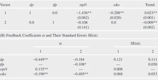
Panel B presents the two cointegrating vectors normalized on (domestic) patent filings and TFP, respectively. We interpreted the two vectors as a knowledge pro-duction function and a function for the determinants of TFP. Panel C reports the feedback coefficients and their standard errors associated with each long-run equation for the variables of the system in first differences.

The cointegrating vectors or relationships as they appear are not uniquely identified and hence the standard errors of these vectors cannot be computed. Any linear combination of the two vectors forms another stationary vector, so the esti-mates produced by any particular vector are not necessarily unique. Therefore, to achieve identification, it is necessary to impose restrictions on the cointegrating vectors. The restrictions are motivated by economic theory and enable us to test for overidentification and obtain standard errors for the overidentified parameters. For ease of exposition and to more easily understand the nature of the restric-tions, the model can be written in terms of equation (16). The error term and short-run components are omitted to focus on the long-term model. Also, the trend is restricted to lie in the cointegration space.

(18)

The βs and αs are those reported in Panels B and C, respectively, in Table 2. These are the implied unrestricted long-run (cointegrating) solutions. The implied (unrestricted) long-run solution of the model is given by the following:

Two restrictions are required to just-identify the model; any additional restric-tions are overidentified and thus testable. The first restriction is on the knowledge tfp=β₂₁dp+β₂₃ stpl1+β₂₄ s&e+β₂₅ Trend. (19) dp=β12 tfp+β13 stpl1+β14 s&e+β15Trend (18) ∆ ∆ ∆ ∆ dp tfp stpl s e t t t t 1 11 12 21 &             = α α α α α α α α α β β β β 31 41 22 32 42 12 13 14 1             − − − − 115 21 23 24 25 1 1 1 1 − − − −     − − β β β β dp tfp stpl t t t−− −                 1 1 17 s e trend t & . ( )

Table 2. Cointegration Analysis of the Data

(A) Johansen’s Cointegration Test

Eigen-Values Null Hypothesis Trace Statistic p-Value

0.937 r =0 183.03** [0.000]

0.687 r ≤1 58.87 ** [0.000]

0.120 r ≤2 6.65 [0.993]

0.019 r ≤3 0.88 [0.997]

(B) Estimated Cointegrating Vectors β′

Vector dp tfp stpl1 s&e Trend

1 1 −0.255 −1.415 −0.195 0.025

2 0.170 1 −0.418 −0.106 −0.002

(C) Feedback Coefficients αand Their Standard Errors SE(α)

α SE(α) 1 2 1 2 dp −0.398 −0.342 0.120 0.121 tfp 0.062 −0.109 0.050 0.050 stpl1 0.132 0.022 0.008 0.008 s&e −0.162 −0.402 0.071 0.072 Notes:

(1) The VAR includes a single lag on each variable (dp, tfp, stpl1,s&e), a constant, trend, and three dummy variables:Stepdum86,Impluse9495, and Impulse96. The estimation sample is 1953 to 1997.

(2) * and ** indicate rejection of the null hypothesis at the 5 percent and 1 percent critical values, respectively.

(19)

production relation and relates the dependence of new knowledge on the stock of knowledge and the R&D scientists and engineers. There does not seem to be a rea-son to include a direct effect from TFP, in this relation, from the R&D-based growth theory. We impose β12=0. Second, the literature does not suggest that cur-rent patent applications should determine productivity. This restriction is imposed by setting β21=0.

The above two restrictions produce a just-identified model. We consider and test three overidentifying restrictions on the βs and αs. The first type of test is for the specification of the cointegrating relation and the latter are tests for weak exogeneity.

First, scientists and engineers in the R&D sector are unlikely to have a direct long-run impact on TFP. Again, the effect is only indirect: R&D scientists and engi-neers produce new knowledge. New knowledge ultimately augments the stock of knowledge and the latter has a potential impact theoretically on tfp. Thus, we exclude s&efrom the second cointegrating vector by testing β24 =0. Statistically, the likelihood ratio test of the restriction β24=0 cannot be rejected. The test statis-tic is χ2₍₁₎=_{1.43 [0.23]; the degrees of freedom are in parentheses and the}_p_-value is in brackets.

Weak exogeneity is an important issue in model reduction. It implies that infer-ence testing can be conducted for the parameters of interest from a conditional den-sity rather than a joint denden-sity without loss of information. The modeling effort is simpler yet still efficient. The first hypothesis is that the cointegrating relationship for new patent flows (dpt) does not explain changes in TFP (∆tfpt). The restriction is α21=0. The “discovery” of new knowledge is unlikely to explain fluctuations in productivity. Our second hypothesis is that TFP does not provide information about the change in the (lagged) stock of knowledge. The timing issue aside, it suggests that stpl1 is weakly exogenous with respect to the second cointegrating vector. Because α32=0, the second cointegrating relationship does not enter the equation for ∆stpl1t. These two feedback coefficients appear numerically small in Panel C of Table 2. If all three overidentifying restrictions are imposed, the joint hypothesis cannot be rejected:χ2₍₃₎=_{4.05 [0.26].}

Restricted Cointegration Model

Table 3 contains the results from the three restrictions on the just-identified model. The table is divided into two panels. Panel A reports the restricted (and identified) estimates for the cointegrating vectors, the βs, together with their standard errors. Panel B reports the feedback coefficients estimates,αs, and their standard errors. In Panel A, the first cointegrating vector is interpreted as a long-run knowledge or “idea” production function. The implied long-run or cointegrating relationship is given by the following:

The coefficient of the lagged stock of knowledge,stpl1, is highly significant and indicates the presence of positive spillovers of knowledge or a standing-on-shoulders dp=1 436. **stpl1 0 208+ . ** &s e−0 023. **Trend. (20))

(20)

effect. The sign of the coefficient is consistent with the R&D-based growth mod-els of Romer (1990) and Jones (1995a). However, its magnitude is significantly greater than unity, indicating a stronger degree of spillovers than the theoretical models.12_{After the second cointegrating vector has been examined, this result will} be discussed further.

The productivity of researchers, s& e,increases with the stock of cumulated knowledge discovered by others in the past. The coefficient of s & eis positive, highly significant, and less than unity. Our estimate of 0.21 is within the range 0.1 to 0.6 that Kortum (1993) finds in the microliterature on patents and R&D effort. It supports Jones’s (1995a) argument for decreasing returns owing to duplicative research. Duplication itself is not wasteful. Replication is an essential exercise in science and a component of learning by doing.

The negative coefficient for the time trend may at first seem surprising. However, it reflects the fact that the number of R&D scientists and engineers grew at a much higher average annual rate than domestic patent applications over the period 1948–97; the growth rate of the former is 4.3 percent and the latter is 1.7 percent. Their difference roughly matches the coefficient of the trend term (−2.3 percent). The negative coefficient of the trend term is also consistent with 12_{In fact, the likelihood ratio statistic rejects the null hypothesis that that coefficient is unity:}χ2₍₁₎= 29.12 [0.00].

Table 3. Restricted Cointegration Analysis of the Data

(A) Cointegrating Vectors β′and Their Standard Errors (in parentheses)

Vector dp tfp stpl1 s&e Trend

1 1 0.0 −1.436** −0.208** 0.023**

(0.062) (0.020) (0.001)

2 0.0 1 −0.108 0.0 −0.009**

(0.141) (0.002)

(B) Feedback Coefficients αand Their Standard Errors SE(α)

α SE(α) 1 2 1 2 dp −0.449** −0.184 0.121 0.111 tfp — −0.108* — 0.050 stpl1 0.135** — 0.008 — s&e −0.190** −0.405** 0.068 0.053 Notes:

(1) The VAR includes a single lag on each variable (dp, tfp, stpl1,s&e), a constant, trend, and three dummy variables:Stepdum86,Impluse9495, and Impulse96. The estimation sample is 1953 to 1997.

(2) * and ** indicate the rejection (at the 5 percent and 1 percent critical values) of the null hypothesis that a particular coefficient is zero. These tests are based on the likelihood ratio statistic, which is distributed under the null hypothesis as χ2_{with 1 degree of freedom.}

(21)

findings by Griliches (1990) based on microdata of patents and R&D. He inter-prets the negative trend as capturing a decrease in the propensity to patent inven-tions because of the rising cost of dealing with the patent system.

Now consider the feedback coefficients for the first cointegrating vector (the knowledge production function) in Panel B of Table 3. They are all significant from zero; this means that dp, stpl1, and s&e are not weakly exogenous with respect to the parameters of the knowledge production function. That is, in the face of any deviation from long-run equilibrium,dp, stpl1, and s&e jointly respond and move the system back to equilibrium. This finding supports our system approach to estimating the knowledge production function. If a single equation approach had been adopted instead, we would have invalidly conditioned on stpl1 and s&e;the result would have produced biased and inconsistent estimates of the knowledge production function.

The feedback coefficient for the ∆dpequation—that is,α11in equation (17)— is −0.45 and significant from zero, suggesting stability of the error correction mech-anism. The coefficient implies that a positive deviation of dpfrom its long-run path, given by equation (20), in this period is not permanent, leading to explosive growth. The growth in (domestic) patent filings declines in the next period.

The feedback coefficient for the ∆stpl1 equation—that is, α31 in equation (17)—is positive and significant from zero. The positive sign suggests that if dpis above its long-run equilibrium path, then this has a positive effect on the growth of the stock of knowledge in the next period.

Finally, the feedback coefficient for the ∆s&eequation—that is,α41in equa-tion (17)—is negative and significant from zero. The negative sign of the coeffi-cient makes sense; it implies that if dpis above its long-run equilibrium path this period, then the growth of the R&D scientists and engineers slows down in the next period to correct for the disequilibrium. This is consistent with the theory that, on a balanced growth path, the proportion of the labor force devoted to knowledge production should remain constant.

Next, consider the second cointegrating vector in Panel A of Table 3. The implied long-run cointegrating relationship is given by the following:

That is, TFP growth depends positively on the lagged stock of knowledge and a time trend. The positive coefficient for the trend term is highly significant and implies a trend growth of TFP of about 1 percent, roughly matching its average annual growth rate over the sample 1948–97. The coefficient for the lagged stock of knowledge is positive but small. It implies that doubling the stock of knowledge will increase TFP by only about 10 percent in the long run. The coefficient actually matches that found by Porter and Stern (2000) for aggregate data on Organization for Economic Cooperation and Development (OECD) countries and falls within the range of estimates of 0.06 to 0.2 found by Griliches (1990) in the micro-productivity literature.

However, the coefficient is not significant. The likelihood ratio statistic under the null hypothesis that the coefficient is zero yields the following: tfp=0 108. stpl1 0 009+ . **Trend. (21)

(22)

χ2₍₁₎= _{0.62 [0.43]. This result is consistent with the insignificant estimates of} R&D on TFP obtained by Jones and Williams (1998) for a panel of U.S. sectors using a fixed effects model. It is also consistent with the Bureau of Labor Statistics (1989) whose growth accounting computation found little contribution of R&D to TFP growth for the U.S. economy, and with Comin (2004) who cal-ibrates a small effect of R&D on productivity using an endogenous growth model with a free entry condition into the R&D sector.

One possible interpretation from Porter and Stern (2000) is that realizing the full benefits from new knowledge and new technologies depends critically on the diffusion of these technologies into the productive sector of the economy. They pro-vide some epro-vidence that the rate of diffusion of new technologies has been slow and incomplete in the OECD countries over the past 20 years. This may explain the weak relationship between the stock of knowledge and TFP. In fact, this idea is sup-ported by or appears to be evident in the U.S. data depicted in Figure 3. Since the mid-1980s, it does not look like the benefits of knowledge have been realized into measured productivity growth. Kortum (1997) identifies the trend shift in patenting behavior. We suspect that the diffusion process of this trend in knowledge growth did not have its full effect on TFP until the late 1990s, just beyond our sample.

The cointegrating relation for TFP enters into the ∆tfpt equation with the appropriate sign and is significant. The feedback effect is rather quick. Changes in scientists and engineers, ∆s&et, are not weakly exogenous as well. If tfpis above

1950 1955 1960 1965 1970 1975 1980 1985 1990 1995 2000 4.0 4.2 4.4 4.6 4.8 5.0 tfp stpl1

Sources: Bureau of Labor Statistics; U.S. Patent and Trademark Office. Note: The series are adjusted by their means.

Figure 3. Total Factor Productivity and (Lagged) Stock of Total Patents

(23)

the long-run level, it reduces s&egrowth over several years. There is less demand for knowledge-producing workers. This has a negative effect on changes in patents,

∆dpt, and is seen in the marginally significant feedback coefficient as well. The stock of knowledge is weakly exogenous with respect to the tfpcointegrating rela-tion. We are not as confident in the interpretation of the feedback coefficients from the TFP relation, because the relationships are perhaps more complex and there is not as much direction from economic theory.

IV. Discussion

This section focuses on two important results mentioned above. The first is the estimated long-run impact of the lagged stock of total patents on domestic patents. This is the coefficient of stpl1 in equation (20), which governs the magnitude of knowledge spillovers. The coefficient is 1.4, significantly greater than unity. The second result is the estimated long-run impact of the lagged stock of total patents on TFP. This is the coefficient of stpl1 in equation (21), which is 0.108.

The microliterature on patents and R&D has little to say on knowledge spillovers, because the knowledge production function from that literature does not derive from the R&D-based models of growth and therefore does not include the stock of existing knowledge as a variable explaining new knowledge. Also, simple aggregation from the microlevel may not capture the potential externalities across sectors.

However, we can compare our results with Porter and Stern (2000). They employ aggregate panel data on OECD countries to estimate a knowledge pro-duction function, in which domestic patents in each country do depend on that country’s existing stock of knowledge. However, they use the stock of domestic patents for a particular country as the proxy for the stock of knowledge in that country, rather than using the stock of total (domestic and foreign) patents, which we use for the U.S. economy. Their results indicate a spillover coefficient of unity supporting the Romer (1990) model.

To check the robustness of our model, we reestimate a knowledge production function, but replace the stock of total (domestic and foreign) patents with the stock of domestic patents. To explain, let sdpl1 denote the (lagged) stock of domestic patents in the U.S. economy. Starting from an unrestricted VAR that includes dp, tfp, sdpl1, and s&e, we implement the Johansen (1988 and 1991) cointegration methodology and again estimate two cointegrating vectors. We find that the esti-mated long-run impact of the (lagged) stock of domestic patents on the flow of new domestic patents (dp) is unity and significant, but the long-run impact of the (lagged) stock of domestic patents on TFP still is small and insignificant (the co-efficient is 0.1 with a standard error of 0.1). We also find, as in equation (21), the trend term to be highly significant in explaining TFP (the coefficient is 0.009 with a standard error of 0.001). For more detailed results, see Abdih and Joutz (2005).

The result that the impact of the (lagged) stock of domestic patents on the flow of new domestic patents is unity is consistent with Porter and Stern (2000) and Romer (1990). This result supports the coefficient of 1.4 on stpl1 in equation (20): When the stock of total (domestic +foreign) patents is used to measure the stock

(24)

of knowledge, researchers have a larger pool of knowledge to draw on, therefore the spillover effect is stronger than the case in which the stock of domestic patents is used.13

We still need to reconcile these results with the time-series evidence presented by Jones (1995b). Romer’s (1990) model assumes a spillover parameter of unity with the implication that the growth rate of the stock of knowledge is proportional to the R&D scientists and engineers. Jones (1995b) directly measured the stock of knowledge using TFP and rejected Romer’s (1990) assumption of a spillover parameter of unity on the basis of the observed weak relationship between TFP growth and the number of R&D scientists and engineers: The number of R&D sci-entists and engineers has been trending strongly upward over the postwar period with no apparent benefit in terms of faster TFP growth. Jones argued that this weak relationship is therefore an indication of weak knowledge spillovers.

The empirical results presented in this paper suggest that once patents are used to measure knowledge, and hence the knowledge production function is directly estimated, the knowledge spillover parameter is unity or larger. That is, R&D sci-entists and engineers appear to have greatly benefited from the knowledge and ideas discovered through prior research. Therefore, the observed weak relationship between TFP growth and R&D scientists and engineers documented by Jones is not necessarily inconsistent with the presence of large knowledge spillovers once knowledge is measured using patent statistics.

The results of this paper point to an alternative explanation of this weak rela-tionship: The knowledge that R&D scientists and engineers produce, as proxied by the patent stock, seems to have had only a limited impact on measured TFP. But why is this so? One possible interpretation is that knowledge is what ultimately matters for growth. Patents may be an imperfect proxy for knowledge, and this is why the effect of patents on TFP is insignificant. In other words, measurement error in the patent stock may be driving this result.14_{In a simple OLS-type} regres-sion, measurement error could bias the estimated coefficient of the patent stock downward and reduce its precision. However, in a dynamic approach like that of

13_{In Romer (1990), Grossman and Helpman (1991b), and Aghion and Howitt (1992), R&D is the sole} source of long-run growth. Although these models are consistent with the large intertemporal knowledge spillovers found in this paper, they are probably inconsistent with the fact that the trend term is highly sig-nificant in explaining TFP, in the sense that the trend may be capturing variables or innovations (apart from those associated with R&D) that influence TFP.

14_{Measurement error could arise because not all knowledge is patentable or will be patented. For} exam-ple, firms may use secrecy as an alternative means of appropriation. Measurement error could also arise because our patent measure does not account for changes over time in the distribution of average patent quality. We are aware that patents are heterogeneous in how much they contribute to knowledge. An ideal measure would probably weigh patents by their “importance” or “quality.” The work of Jaffe, Trajtenberg, and Henderson (1993) and Jaffe, Trajtenberg, and Fogarty (2000) has attempted to do that at the microlevel, usually for a sample of patents in a cross-sectional framework. Patent citations have been used as a mea-sure of quality or importance in that work. However, to our knowledge, there has been no attempt to address or measure how the distribution of patent quality has evolved at the aggregate level over time for the entire postwar period in the United States. The data are simply not available. This probably explains why virtu-ally all aggregate growth studies that use patents as an indicator of technology/knowledge have relied on patent counts following the tradition of Griliches (1990). Our paper follows this tradition.