This item was submitted to Loughborough’s Institutional Repository
(
https://dspace.lboro.ac.uk/
) by the author and is made available under the
following Creative Commons Licence conditions.
For the full text of this licence, please go to:
http://creativecommons.org/licenses/by-nc-nd/2.5/
A binary decision diagram method for phased
mission analysis of non-repairable systems
S J DunnettandJ D Andrews*Department of Aeronautical and Automotive Engineering, Loughborough University, Loughborough, UK
The manuscript was received on 9 March 2006 and was accepted after revision for publication on 19 May 2006.
DOI: 10.1243/1748006XJRR27
Abstract: Phased mission analysis is carried out to predict the reliability of systems which undergo a series of phases, each with differing requirements for success, with the mission objective being achieved only on the successful completion of all phases. Many systems from a range of industries experience such missions. The methods used for phased mission analysis are dependent upon the repairability of the system during the phases. If the system is non-repairable, fault-tree-based methods offer an efficient solution. For repairable systems, Markov approaches can be used.
This paper is concerned with the analysis of non-repairable systems. When the phased mission failure causes are represented using fault trees, it is shown that the binary decision diagram (BDD) method of analysis offers advantages in the solution process. A new way in which BDD models can be efficiently developed for phased mission analysis is proposed. The paper presents a methodology by which the phased mission models can be developed and analysed to produce the phase failure modes and the phase failure likelihoods.
Keywords: phased mission analysis, fault tree analysis, binary decision diagrams, non-repairable systems
1 INTRODUCTION
Many systems undergo phased missions when per-forming the functions for which they are designed. A phased mission is one where the overall mission can be split into a number of phases, performed in sequence, in which the objectives change from one phase to the next. The mission is successfully com-pleted if all phases are successfully accomplished. For example an aircraft flight could be considered as a mission with phases: taxiing to the runway, take-off, ascend to the correct altitude, cruise, des-cend, land, and taxi back to the terminal. Each phase uses differing functional elements of the system and so the causes of failure in each phase will be different.
In such circumstances, mission reliability can-not be determined by studying the individual phases of the mission in isolation, for two reasons.
1. The phase failure probabilities are not statisti-cally independent. Some components or subsys-tems influence the success, or failure, of more than one phase.
2. It cannot be assumed that all components are functioning at the start of each phase, even if they can be assumed functional at the start of the mission. In the example of an aircraft flight, if the landing gear fails following take-off during the ascend, cruise, or descend phases, it will remain that way until the landing phase, when the mission will fail. Failures can remain unre-vealed in some phases and mission failure will occur not when the failure events happen but on the point of transfer from one phase to another.
The methods for conducting systems reliability assessments for phased missions utilize different techniques depending on whether the system can
*Corresponding author: Department of Aeronautical and Automotive Engineering, University of Loughborough, Lough-borough, Leicestershire LE11 3TU, UK. email: J.D.Andrews@ lboro.ac.uk
be repaired or not. For systems which are non-repairable throughout the duration of the mission, such as an aircraft flight, fault tree methods offer the most efficient solution. Esary and Ziehms [1] used fault trees to represent the failure conditions for each mission phase which can be combined and, with the use of a minimal cut set reduction method, evaluated to obtain the mission unreliabil-ity. A component’s failure during each phase of the mission was considered as a separate event. This sig-nificantly increases the size of the problem for analy-sis. Zang et al. [2] extended the fault-tree-based method to utilize binary decision diagrams (BDDs) as a more effective representation of the phase failure logic for efficient analysis.
By considering the failure of each phase individu-ally, the problem complexity can be reduced [3]. The conditions for a failure in any specified phase occur when all previous phases have completed suc-cessfully, and then either the failure conditions occur, causing in-phase failure, or the failure condi-tions already exist when the phase is entered, caus-ing phase transition failure. This approach again employs BDDs and develops a new event algebra to account for the non-independence of the compo-nent failure events from one phase to the next. In addition to the overall mission unreliability, the method also yields the phase unreliabilities, which can be used in risk studies where the consequences of failure differ from phase to phase. (For example, consider the consequences of failure in the taxiing phase or the cruise phase of an aircraft flight.)
Where components can fail and be repaired during the mission, Markov methods are used to calculate the mission failure probability [4–6].
The research reported in this paper develops an efficient, systematic generation of the mission BDD for phased missions. While using a single model to represent the conditions for mission fail-ure, as with the method of La Band and Andrews [3], the phase failure probabilities can also be deduced.
2 BINARY DECISION DIAGRAMS
BDDs offer an alternative approach to fault trees to represent a system’s failure logic. Their structure enables the system failure probability to be deduced efficiently and without resort to any approximations. However, they are difficult to construct directly from the system definition and are generally obtained by converting from a fault tree.
A BDD is a directed acyclic graph with all paths starting at the top root vertex and terminating in one of two terminal vertices, 1 or 0. A terminal 1 ver-tex indicates top event occurrence, and a terminal 0 vertex indicates top event non-occurrence. The dia-gram consists of terminal and non-terminal vertices connected by branches; the non-terminal vertices correspond to basic events. Each non-terminal ver-tex has two branches leaving it, a 1 branch and a 0 branch, which indicate occurrence and non-occur-rence respectively of the basic event. The construc-tion of the BDD requires the basic events to be ordered. In Fig. 1 an example of a BDD is shown: it represents the logic function A.BþB.C with the orderingA<B <Cassumed (note that the symbol
þ represents logical OR, and the symbol . repre-sents logical AND).
A B B C 1 0 1 0 0 1 0 1 0 1 0 1 0 Root Vertex Terminal 0 vertex Non-terminal vertex Fig. 1 BDD
Paths through the BDD indicate the component conditions which determine the system state as given by the terminal node. So, in the BDD shown in Fig. 1, ifA fails and B fails, a terminal 1 node is reached, which means that, under these conditions, system failure occurs (i.e. this specifies a cut set).
3 BINARY DECISION DIAGRAM CONSTRUCTION
The conventional rules used for constructing BDDs from fault trees have been covered extensively in previous papers [7, 8] and will therefore only be summarized here. From the structure of the BDD shown in Fig. 1 it can be seen that each intermediate node can be represented as an if–then–else (ite) triple of the form
iteðX,f1,f2Þ ð1Þ
whereX is a Boolean variable, f1is a logic function
to consider if X is true (on the 1 branch) andf2 is
a logic function to consider if X is false (on the 0 branch). When combining two logic functions expressed in this way, the rules are as follows: if
h¼iteðX,h1,h2Þ and k¼iteðY,k1,k2Þ are two logic functions, then
hk¼ iteðX,h1k1,h2k2Þ, X¼Y
iteðX,h1k,h2kÞ, X <Y
ð2Þ whererepresents the AND/OR logic operator.
The method used for constructing the BDDs in this paper is one whereby the BDDs for each phase in the mission can be constructed separately and then combined to form the mission BDD. It is accomplished by noting the structures which result when inputs for each gate type are combined.
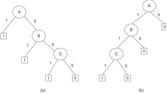
For example, consider the BDDs representing the logic expressions AþBþC and A.B.C shown in Figs 2(a) and (b) respectively, where the ordering
A<B<Chas been assumed.
For an OR gate the BDD structure forms a chain where the basic events are linked by their 0 branches. The AND gate BDD structure has the basic events linked on their 1 branches. This concept can also be extended to combining logical expressions which are inputs to fault tree gates. For example, if h and k are logic expressions which are inputs to an OR gate, then the BDD representing the combined logical expression can be obtained by replacing the terminal 0 vertices in the BDD senting the first logical expression by the BDD repre-senting the second logical expression. For inputs to an AND gate, each terminal 1 vertex is replaced by the second BDD. Once the combined BDD is formed, prior to simplification, it is possible that the ordering assigned to the basic event variables will be destroyed and some variables may appear more than once on paths from the root vertex to the terminal nodes. Care must then be taken to deal with repeated variables on the same path. If by combining BDDs there is now, in the new BDD, a variable which also appears earlier in the structure, this repeated variable can be removed. The first occurrence of the variable is the one which fixes its state. So, if on some path a variable is first passed through on its 1 branch, this fixes that the component is in its failed state on this path. For the second occurrence, the node is omitted and replaced with a link directly to the node on its 1 branch; every-thing below its 0 branch is deleted. If the path first passes the basic event on its 0 branch, the com-ponent failure has not occurred on this path, the second occurrence of the node is replaced by a
A B C 1 1 1 0 A B C 1 0 0 0 1 0 1 0 1 0 1 0 1 0 1 0 (a) (b)
direct link to the node on its 0 branch, and the nodes connected to the 1 branch are deleted. The following standard collapsing operations can also be applied to obtain the most efficient BDD.
1. If the two sons of a node Xare equivalent, then delete node X and direct all its incoming edges to its left son.
2. If nodesAandBare equivalent, then delete node
Band direct all its incoming edges toA.
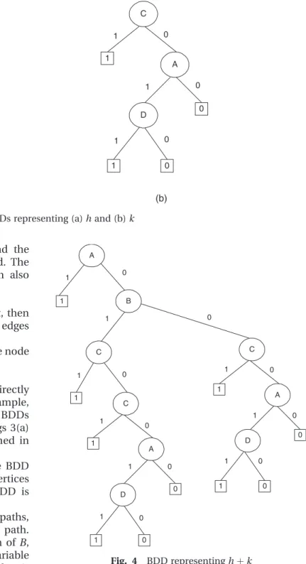
A ‘son’ of a node is simply the node directly attached to either its 1 or 0 branch. For example, consider h¼AþB.C and k¼CþA.D; the BDDs representing these functions are shown in Figs 3(a) and (b), with the ordering A < B < C assumed in the first BDD andC<A<Din the second.
To obtain the BDD representing hþk, the BDD representingk replaces the two terminal 0 vertices in the BDD representing h. The resulting BDD is shown in Fig. 4.
As can be seen, variables are repeated on paths, e.g. both A and C are repeated on the same path. Considering the path 0 branch ofA, 1 branch ofB, and 0 branch ofCtakes us to the repeated variable
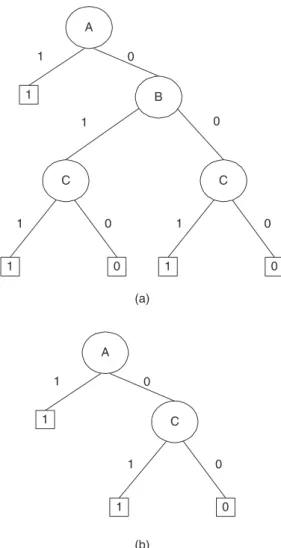
C. As this lies on the 0 branch ofC, the repeated vari-able can be removed and all that lies on its 0 branch kept. This then leads to the repeated variable A; as this lies on the 0 branch of the first occurrence of A, the repeated variable can be removed and all that lies on its 0 branch kept. This is just a term-inal 0 vertex. The other repetition ofA can be dealt with in the same manner. The resulting BDD is shown in Fig. 5(a). By identifying that the variable
B is irrelevant, the final, reduced BDD is shown in Fig. 5(b).
This method of combining BDDs can be adopted to model phased mission problems efficiently. The
methodology to do this will be developed and demonstrated by considering a simple example.
4 PHASED MISSION EXAMPLE
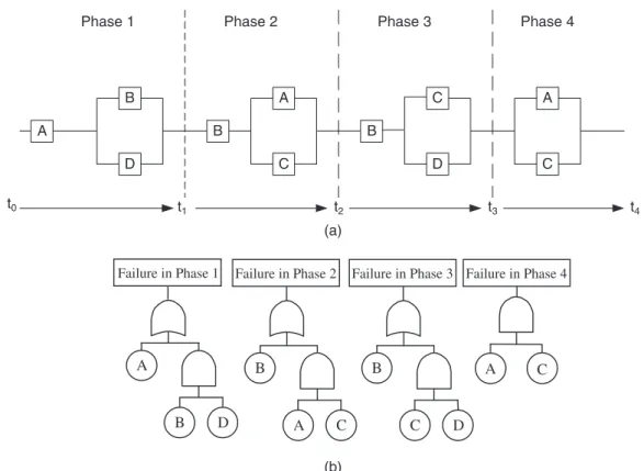
A simple phased mission problem consisting of non-repairable components A, B, C, and D (Fig. 6(a)), will be considered here in order to demonstrate an efficient method of BDD construction for phased mission analysis. A B C 1 0 1 0 C A D 1 0 0 1 1 0 1 0 1 0 1 0 1 0 1 0 (a) (b)
Fig. 3 BDDs representing (a)hand (b)k
A B C 1 1 C A D 1 0 0 1 C A D 1 0 0 1 1 1 1 1 1 1 1 1 1 0 0 0 0 0 0 0 0 0 Fig. 4 BDD representinghþk
During phase 1, which lasts until timet1, the
suc-cess of the mission is dependent upon the fact that componentAand at least one of componentsB
and D functions. Successful completion of phase 1 means that the mission then enters phase 2, which requires componentBand at least one of components
AandCto function between timest1andt2.
Success-ful completion of that phase then means that the sys-tem enters phase 3, and so on. The mission is successfully accomplished if all phases are completed successfully.
The phase failure fault trees are given for this mission in Fig. 6(b).
5 CONSTRUCTION OF PHASE BDDs
The first stage in the methodology is to convert all the phase fault trees to their BDD form. Considering phase 1, the top event, ‘failure in phase 1’ is given by the logical expressionA1þB1.D1, where the notation
Ai represents the failure of componentAin phasei.
Assuming the orderingA1<B1<D1, and using the
rules that for the OR gate the events are linked by their 0 branches and for an AND gate by their 1 branches, the BDD representing this expression is shown in Fig. 7(a). In phased mission problems the state of components which are used in subsequent phases are important, as they have a bearing on the future performance of the system. Hence, in the BDDs representing each phase, paths ending in a terminal 0 vertex, representing system functioning through that phase, must consider all components used in that and subsequent phases. Therefore the BDD representing failure in phase 1, shown in Fig. 7(a), must be extended so that all component states are defined on the paths ending in a terminal 0 vertex where the mission will pass to the next phase. On the terminal 0 connected to nodeB1, the
condi-tions of A1 and B1 are specified (both work). This
needs to be expanded to include all states that componentsC1andD1can reside in. For the second
terminal 0 (the 0 branch of theD1node) the status
of A1, B1, and D1 is fixed. It only remains to
con-sider all states for C1. The extended BDD is shown
in Fig. 7(b).
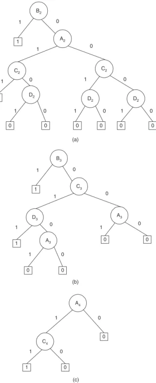
The BDDs developed for failure of the other three phases are illustrated in Fig. 8.
The ordering of basic events can be different for each phase (as it is in this example) to obtain the most efficient representation of the phase failure logic.
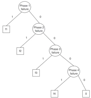
6 CONSTRUCTION OF THE MISSION BDD These BDDs representing failure on the separate phases will now be used to construct a mission BDD. The overall structure of the mission BDD is shown in Fig. 9. There are now more than two sys-tem outcomes identified, which means that this new failure logic structure departs subtly from the BDD. The end states represent either a failure in a phase, labelledf1,f2,f3, orf4for failure in the phase
indicated, or a mission success, labelled 0.
Once constructed, the BDD can then be subjected to a reduction process to ensure that the component state logic is consistent on any branch.
The resulting BDD can be reduced by use of the following rules.
Rule 1.Ai:Aj ¼0, as a non-repairable component A
cannot fail in phaseiand phasej.
Rule 2. Ai:Aj ¼0 fori<j, as a component cannot
be repaired once failed.
Rule 3. IfK1is a minimal cut set for phasej, and the
components which make up this cut set fail in phases prior to j, then upon entering phase j the system will fail.
A C 1 1 0 1 1 0 0 1 0 B C 1 0 1 0 A C 1 1 0 1 1 0 0 (a) (b)
Ai represents the fact that component A functions
throughout phasei. The system example illustrated in Fig. 6 is considered again to demonstrate the con-struction process. The BDDs shown in Figs 7(b) and 8(a), representing failure in phases 1 and 2 can be combined into a single BDD representing failure in phases 1 or 2 by replacing the terminal 0 vertices in the BDD in Fig. 7(b) with the BDD in Fig. 8(a). The resulting BDD is shown in Fig. 10(a). This has been reduced using the rules 1 to 3 above.
Apply rules 1 and 2 along the following paths: 1. along the 0 branch ofA1, 0 branch ofB1, 1 branch
of D1, 1 branch of C1, 0 branch of B2, and 1
branch ofA2;
2. along the 0 branch of A1, 0 branch of B1, 0
branch ofD1, 1 branch ofC1, 0 branch ofB2, and
1 branch ofA2.
In both cases, remove node C2 and connect
directly to f2, as component Chas already failed in
phase 1.
Similarly, apply rules 1 and 2 to the following paths:
1. along the 0 branch of A1, 0 branch of B1, 1
branch ofD1, 1 branch ofC1, 0 branch ofB2, and
0 branch ofA2;
2. along the 0 branch of A1, 0 branch of B1, 1
branch of D1, 0 branch of C1, 0 branch of B2, 1
branch ofA2, and 0 branch ofC2;
3. along the 0 branch ofA1, 0 branch ofB1, 1 branch
ofD1, 0 branch ofC1, 0 branch ofB2, 0 branch of
A2, and 1 branch ofC2;
4. along the 0 branch ofA1, 0 branch ofB1, 1 branch
ofD1, 0 branch ofC1, 0 branch ofB2, 0 branch of
A2, and 0 branch ofC2.
This results in a terminal 0 vertex.
Applying rules 1 and 2 to the path, 0 branch ofA1,
0 branch of B1, 0 branch of D1, 1 branch of C1,
0 branch of B2, and 0 branch of A2 removes C2.
Applying rule 3 to the path, 0 branch ofA1, 1 branch
ofB1, and 0 branch ofD1results in the terminal node
f2, asBis a single order minimal cut set for phase 2.
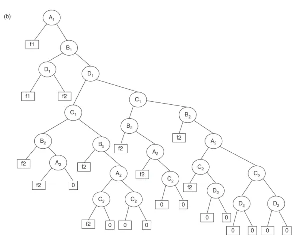
The resulting reduced BDD is shown in Fig. 10(b), where the 1 and 0 labels on the branches leaving each intermediate node have been omitted for clarity. This BDD was then combined with the BDD representing failure in phase 3 (the phase 3 BDD is attached to the 0 branches of the combined phase 1 and 2 BDD) and reduced, using rules 1 to 3, to obtain a single BDD representing failure in phase 1, 2, or 3. The resulting BDD has 47 outcomes of which 31 are failures, two are failure in phase 1, nine are failure in phase 2, and 20 are failure in phase 3. Combining this BDD with the BDD senting failure in phase 4, (Fig. 8(c)), the BDD repre-senting mission failure is obtained. This is shown in Fig. 11, where the 1 and 0 labels on the branches leaving each intermediate node have again been A D B B A C B C D A C Phase 1 (a) (b)
Phase 2 Phase 3 Phase 4
t0 t1 t2 t3 t4 Failure in Phase 1 A B D Failure in Phase 2 B A C Failure in Phase 3 B C D Failure in Phase 4 A C
Fig. 6 (a) Reliability network of a simple phased mission system; (b) fault tree representation of individual phase failures
omitted for clarity. Each left edge leaving a variable node is the ‘1 branch’ and each right edge the ‘0 branch’. In this case there are 47 failure outcomes; two in phase 1, nine in phase 2, 20 in phase 3, and 16 in phase 4. This is equivalent to the results obtai-ned using the cause consequence diagram method for this problem [9]. This method of combining the BDDs for the different phases can obviously be applied to any phase mission problem for a non-repairable system, but in order to demonstrate how the method is applied has been shown here for the particular example taken.
7 QUANTIFICATION 7.1 Phase failure modes
Each path through the mission BDD will termin-ate in either a phase failure or the mission success. The component status conditions encountered
along each path will specify over which phases the components must work and which phase it is possi-ble for the failure to occur in order to cause the spe-cified system event. From the path conditions which result in system failure in any phase the phase failure modes can be determined. A phase failure mode is a list of the necessary and sufficient conditions experi-enced at component-level events (phases working and phases where failure can occur), which lead to the specified phase failure.
A1 1 B1 D1 1 0 0 1 1 1 0 0 0 A1 1 B1 D1 1 C1 0 0 D1 C1 0 0 C1 0 0 1 1 1 1 1 0 0 0 0 1 0 1 0 0 (a) (b)
Fig. 7 BDDs representing failure in phase 1
B2 A2 C2 C2 D2 D2 D2 1 1 0 0 0 0 0 0 1 0 1 0 1 0 1 1 1 1 0 0 0 0 (a) (b) (c) B3 C3 D3 A3 A3 1 1 0 0 0 0 1 0 1 1 1 1 0 0 0 0 A4 C4 1 0 0 1 1 0 0
Fig. 8 BDDs representing failure in (a) phase 2, (b) phase 3, and (c) phase 4
For systems with non-repairable components it is possible to introduce a phase algebra to deter-mine the phase failure modes. This algebra was established in reference [3]; it will account for the non-independence of component conditions from one phase to the next, and enable the minimal con-ditions required for phase failure to be established, which will be used in the phase failure probability calculations. It is only of interest in which phases the component failure could occur to contribute to the phase failure. When considering the disjoint paths for phased mission systems with non-repairable components, account must be taken of the fact that, if a component fails in phasei, then it must have worked through phases 1,. . .,i1. This is expressed algebraically as
A1,i1:Ai¼Ai ð3Þ
whereAj,krepresents the functioning of component
Afrom the start of phasejto the end of phasek. Using rules 1 and 2 from the section on construc-tion of the mission BDD with the condiconstruc-tion
Ai:Ai¼Ai ð4Þ
the phase failure modes can be evaluated. This is illustrated for the first two phases of the mission BDD shown in Fig. 10(b). The disjoint paths leading to failure in phase 1 are
A1
A1:B1:D1
ð5Þ
The initial disjoint paths leading to failure in phase 2 and their subsequent reduction to the phase failure modes are A1:B1:D1 A1:B1:D1:C1:B2!A1:D1:C1:B2 A1:B1:D1:C1:B2:A2!B12:D1:C1:A2 A1:B1:D1:C1:B2!A1:D1:C1:B2 A1:B1:D1:C1:B2:A2:C2!B12:D1:A2:C2 A1:B1:D1:C1:B2!A1:D1:C1:B2 A1:B1:D1:C1:B2:A2!B12:D1:C1:A2 A1:B1:D1:C1:B2!A1:D1:C1:B2 A1:B1:D1:C1:B2:A2:C2!B12:D1:A2:C2 ð6Þ
Phase failure modes for the other phases are eval-uated in the same way; this produces 20 phase 3 failure modes and 16 phase 4 failure modes, which are not listed here.
7.2 Phase and mission failure probability
Each path on a BDD through to a terminalfivertex is disjoint, and therefore the phase failure probability can be obtained by summing the probabilities of the disjoint paths. In order to find the mission failure probability it is necessary to sum the probabilities of all the disjoint paths ending in any terminalfi.
Using the method described in this paper, more information can be gained than just mission failure probability, as the BDD also gives the probability of failure in each phase. This has an advantage over other methods [1], which produce only the mission failure probability.
The example phased mission used to illustrate the method is considered again;qAi is used to represent
the failure probability of component A in phase i, andQiis taken to be the failure probability in phase
i. Then
qAi¼
Zti
ti1
fAðtÞdt ð7Þ
wherefAðtÞ is the failure density function for
com-ponentA in phasei, and phase iruns from ti1 to
ti. For phase 1
Q1¼qA1þð1qA1ÞqB1qD1 ð8Þ
For phase 2 then
Q2¼ð1qA1Þð1qD1ÞqB1þð1qA1ÞqD1qC1qB2 þð1qB1qB2ÞqD1qC1qA2þð1qA1Þð1qC1ÞqD1qB2 þð1qB1qB2ÞqD1qA2qC2þð1qA1Þð1qD1ÞqC1qB2 þð1qB1qB2Þð1qD1ÞqC1qA2 þð1qA1Þð1qD1Þð1qC1ÞqB2 þð1qB1qB2Þð1qD1ÞqA2qC2 f1 f2 f3 f4 0 1 1 1 1 0 0 0 0 Phase 1 failure Phase 2 failure Phase 3 failure Phase 4 failure
0 0 A1 f1 B1 D1 f1 C1 D1 C1 1 0 B2 A2 C2 C2 D2 D2 D2 f2 f2 00 00 0 0 10 1 1 1 1 1 0 00 B2 A2 C2 C2 D2 D2 D2 f2 f2 0 00 0 0 0 1 1 1 1 1 1 1 0 0 00 0 B2 A2 C2 C2 D2 D2 D2 f2 f2 00 000 0 1 1 1 1 1 1 0 00 00 0 0 0 0 0 0 0 1 1 1 1 1 1 0 0 0 0 B2 A2 f2 1 0 C2 D2 f2 00 1 1 1 0 1 0 D2 000 0 1 1 00 1 1 0 B2 A2 C2 C2 D2 f2 f2 00 00 0 0 1 0 1 1 1 1 1 0 00 B2 A2 C2 C2 D2 D2 D2 f2 f2 00 0 0 0 0 1 1 1 1 1 1 0 0 0 00 0 0 0 0 1 0 C1 C2 D2 D2 D2 (a) Fig. 10 (a) BDD representing failure in phases 1 o r phase 2
Expressions can also be determined for Q3 and Q4
using the same method. The probability Qmisson
of the mission failure can then be determined using Qmission¼ X i Qi ð9Þ 8 GENERAL ALGORITHM 8.1 Mission BDD construction
1. Utilizing constructs for AND and OR gates produces the BDD for each phase from the phase fault trees. These are expanded in com-parison with usual BDDs, as all possible states of components required in future stages must be explicitly considered on the paths leading to phase success.
2. By considering the mission failure as an OR combination of the phase failures, a mission BDD can be constructed. Terminal mission BDD nodes denote the phase in which the mis-sion fails or that mismis-sion success has been achieved. Since it has more than two possible outcomes, this mission BDD is subtly different from a conventional BDD.
3. Phase failure BDDs are incorporated, one by one, into the mission BDD to yield a structure where mission states are determined by the per-formance of the components in each phase. 4. The mission BDD is reduced to its simplest form
by removing paths which represent impossible component conditions such as failing more than once or working in phases which follow a failure.
8.2 Mission BDD quantification
1. Failure modes for each phase of the mission are obtained by considering the component condi-tions represented along each of the BDD paths leading to the specified phase failure.
2. The failure modes are simplified using the phase algebra.
3. Component phase failure probabilities are eval-uated.
4. Using the disjoint phase failure modes and the component failure probabilities the phase failure likelihoods are quantified.
5. The phase failure probabilities can be combined with the consequences of phase failure in order to perform a mission risk analysis, or summed to yield the mission failure probability.
A1 f1 B 1 D1 f1 f2 D1 C1 f2 B2 A2 f2 0 f2 B2 A2 f2 C2 0 0 C2 0 C1 B2 f2 A2 0 C2 0 f2 B2 f2 A 2 C2 f2 C2 0 D2 0 0 D2 0 0 D2 0 (b)
A1 f1 B1 D1 f1 f2 D1 C1 f2 B2 A2 f2 f3 f2 B2 A2 f2 C2 f3 C2 C1 B2 f2 A2 f3 D2 f2 B3 f3 C3 f3 C4 f4 0 B3 f3 C3 f3 A3 f4 C4 0 A4 f4 C4 0 0 B3 f3 D3 f3 A3 f4 A3 f4 0 B2 f2 A2 C2 f2 C2 D2 f3 D2 D2 B3 f3 C3 f3 C4 f4 0 B3 f3 C3 C4 f4 0 D3 f3 f4 B3 f3 D3 f4 A3 f3 A4 f4 0 B3 f3 C3 A3 f3 f4 0 A4 C4 f4 0 0 B3 f3 C3 f3 f4 A4 f4 0 A3 A3 C4 f4 0 A4 C4 C4 f4 0 0 D3 Fig. 11 BDD representing mission failure
9 CONCLUSIONS
1. The method given in this paper provides an effective approach for developing the BDD for a system which undergoes a phased mission. This BDD will identify the causes of each phase failure.
2. The phase failure modes can be identified from the resulting mission BDD.
3. Using the disjoint nature of the phase failure modes and the probability of component failures in specified phases, the phase failure probability for each phase can be obtained. This can be combined with differing consequences of failure in any phase to perform a mission risk analysis. 4. Mission failure probability is obtained by
sum-ming the phase failure likelihoods. REFERENCES
1 Esary, J. D.andZiehms, H.Reliability analysis of phased missions. InReliability and fault tree analysis, 1975, pp. 213–236. (Society for Industrial Applied Mathematics, Philadelphia, Pennsylvania).
2 Zang, X., Sun, H.,andTrivedi, K. S.A BDD-based algo-rithm for reliability analysis of phased mission systems.
IEEE Trans. Reliability, 1999,48(1), 50–60.
3 La Band, R.andAndrews, J. D.Phased mission model-ling using fault tree analysis. Proc. Instn Mech. Engrs,
Part E: J. Process Mechanical Engineering, 2004, 218,
83–91.
4 Clarotti, C. A., Contini, S.,andSomma, R.Repairable multi-phase systems – Markov approaches for reliability evaluation. InSynthesis and analysis methods for safety
and reliability studies(Eds G. Apostolakis, S. Garribba,
and G. Volta), 1980, pp. 45–58 (Plenum, New York).
5 Smotherman, M.andZemoudeh, K.A non-homogen-eous Markov model for phase mission reliability analysis.IEEE Trans.Reliability, 1989,38, 585–590.
6 Smotherman, M.andGeist, R. M.Phased effectiveness using a non-homogeneous Markov reward model.
Relia-bility Engng System Safety, 1990,27, 241–255.
7 Rauzy, A.New algorithms for fault tree analysis.
Relia-bility Engng System Safety, 1993,40, 203–211.
8 Sinnamon, R. M. and Andrews, J. D. Improved effi-ciency in qualitative fault tree analysis.Qual. Reliability
Engng Int., 1997,13, 293–298.
9 Vyzaite, G., Dunnett, S.,andAndrews, J. D.Cause con-sequence analysis of non-repairable phased missions.