Stochastic relational processes: Efficient inference and applications

Stochastic relational processes:

Efficient inference and applications

Ingo Thon1, Niels Landwehr2, and Luc De Raedt1

1

Department of Computer Science, Katholieke Universiteit Leuven, Celestijnenlaan 200A, 3001 Heverlee, Belgium

2

Department of Computer Science, University of Potsdam, August-Bebel-Str. 89, 14482 Potsdam, Germany

[email protected], [email protected], [email protected]

Abstract. One of the goals of artificial intelligence is to develop agents that learn and act in complex environments. Realistic environments typically feature a vari-able number of objects, relations amongst them, and non-deterministic transition behavior. While standard probabilistic sequence models provide efficient infer-ence and learning techniques for sequential data, they typically cannot fully cap-ture the relational complexity. On the other hand, statistical relational learning techniques are often too inefficient to cope with complex sequential data. In this paper, we introduce a simple model that occupies an intermediate position in this expressiveness/efficiency trade-off. It is based on CP-logic (Causal Probabilis-tic Logic), an expressive probabilisProbabilis-tic logic for modeling causality. However, by specializing CP-logic to represent a probability distribution over sequences of relational state descriptions and employing a Markov assumption, inference and learning become more tractable and effective. Specifically, we show how to solve part of the inference and learning problems directly at the first-order level, while transforming the remaining part into the problem of computing all satisfying as-signments for a Boolean formula in a binary decision diagram.

We experimentally validate that the resulting technique is able to handle proba-bilistic relational domains with a substantial number of objects and relations.

1

Introduction

One of the current challenges in artificial intelligence is the modeling of dynamic envi-ronments that change due to actions and activities people or other agents take. As one example, consider a model of the activities of a cognitively impaired person [1]. Such a model can be used to assist persons, using common patterns to generate reminders or detect potentially dangerous situations, and thus help to improve living conditions.

As another example and one on which we shall focus in this paper, consider a model of the environment in amassively multiplayer online game(MMOG). These are com-puter games that support thousands of players in complex, persistent, and dynamic vir-tual worlds. They form an ideal and realistic testbed for developing and evaluating ar-tificial intelligence techniques and are also interesting in their own right (cf. also [2]). One challenge in such games is to build a dynamic probabilistic model of high-level

player behavior, such as players joining or leaving alliances and concerted actions by players within one alliance. Such a model of human cooperative behavior can be use-ful in several ways. Analysis of in-game social networks is not only interesting from a sociological point of view but could also be used to visualize aspects of the gaming environment or give advice to inexperienced players (e.g., which alliance to join). More ambitiously, the model could be used to build computer-controlled players that mimic the cooperative behavior of human players, form alliances and jointly pursue goals that would be impossible to attain otherwise. Mastering these social aspects of the game will be crucial to building smart and challenging computer-controlled opponents, which are currently lacking in most MMOGs. Finally, the model could also serve to detect non-human players in today’s MMOGs—accounts which are played by automatic scripts to give one player an unfair advantage, and are typically against game rules.

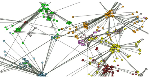
From a machine learning perspective, this type of domain poses three main chal-lenges: 1) the world state descriptions are inherently relational, as the interaction be-tween (groups of) agents is of central interest, 2) the transition behavior of the world is strongly stochastic, and 3) a relatively large number of objects and relations is needed to build meaningful models, as the defining element of environments such as MMOGs are interactions amonglargesets of agents. Thus, we need an approach that is both com-putationally efficient and able to represent complex relational state descriptions and stochastic world dynamics. In this setting, a relation state typically corresponds to a labeled (hyper)graph, and therefore the model can also be viewed as a stochastic model over sequences of graphs, cf. Figure 8.

Artificial intelligence has already contributed a rich variety of different model-ing approaches, for instance, Markov models [3] and decision processes [4], dynamic Bayesian networks [5], STRIPS [6] and PPDDL [7] (see also [8] for a discussion of the relationship between CPT-L and PPDDL), statistical relational learning representa-tions [9], etc. Most of the existing approaches that support reasoning about uncertainty (that is, satisfy requirement 2) employ essentially propositional representations (for instance, dynamic Bayesian networks, Markov models, etc.). Thus, they are not able to represent complex relational worlds, and do not satisfy requirement 1). A class of models that integrates logical or relational representations with methods for reasoning about uncertainty (for instance, Markov Logic [10], CP-logic [11], or Bayesian Logic Programs [12]) is considered within statistical relational learning [9] and probabilistic inductive logic programming [13]. However, inference and learning often cause signif-icant computational problems in realistic applications, and hence, such methods do not satisfy requirement 3).

We want to alleviate this situation, by contributing a novel representation, called CPT-L (for CausalProbabilisticTime-Logic), that occupies an intermediate position in this expressiveness/efficiency trade-off. A CPT-L model essentially defines a proba-bility distribution over sequences of interpretations. Interpretations are relational state descriptions that are typically used in planning and many other applications of artificial intelligence. CPT-L can be considered a variation of CP-logic [11], a recent expres-sive logic for modeling causality. By focusing on the sequential aspect and deliberately avoiding the complications that arise when dealing with hidden variables, CPT-L is

more restricted, but also more efficient to use than alternative formalisms within the artificial intelligence and statistical relational learning literature.

The present paper builds upon our recent work in this area [14], and extends this earlier work in several directions. As a first contribution, we generalize the model pre-sented in [14] to include the case that head elements are conjunctions of atoms rather than individual atoms. Second, we relax the strict Markov assumption employed in the original approach, thus allowing causal influences to stretch over several time steps. Third, we present partially lifted algorithms for inference and learning in CPT-L, and empirically show that they reduce the overall computational complexity of our approach substantially. Finally, we contribute a more detailed and comprehensive experimental evaluation of our approach.

The rest of the paper is organized as follows: Section 2 introduces the CPT-L frame-work; Section 3 addresses inference and parameter estimation; and Section 4 presents experimental results in several (artificial and real-world) domains. Finally, we discuss related work in Section 5, before concluding and touching upon future work in Sec-tion 6. Proofs of the main theorems are contained in the appendix.

2

CPT-L

This section describes the CPT-L model. We begin with a brief review of CP-logic (Causal Probabilistic Logic), and then present the CPT-L model as a variant of the more general CP-logic framework.

2.1 CP-logic

Let us first introduce some terminology. A logicalatomis an expression of the form

p(t1, . . . , tn)wherep/nis apredicate symboland thetiareterms. Terms are built up

from constants, variables, and functor symbols. Constants are denoted in lower case (such asa), variables in upper case (such asZ), and functors byf /k wherek is the arity of functorf. The set of all atoms is called alanguageL.Groundexpressions do not contain variables. Ground atoms will be calledfacts. A substitutionθis a mapping from variables to terms, andbθis the atom obtained frombby replacing variables with terms according toθ. As an example, consider the substitutionθ={Z/a}that replaces variableZwitha, as inbθ=p(a)forb=p(Z).

Complex world states can now be described in terms ofinterpretations. An interpre-tationIis a set of ground facts{a1, . . . , aN}. These ground facts can represent objects

in the current world state, their properties, and any relationship between objects. As an example, consider the representation of the state of a multiplayer game in terms of an interpretation as depicted in Figure 1.

The semantics of our framework is based on CP-logic, a probabilistic first-order logic that defines probability distributions over interpretations [11]. CP-logic is closely related to other probabilistic logic programming systems, such as PRISM [15], ICL [16], and ProbLog [17], that are based on Sato’s distribution semantics [18]. How-ever, CP-logic is more intuitive as a knowledge representation framework. The reason is

Greeks Achilles Menelaos Mykena Sparta Pelion Troy Paris

Trojans city(pelion, achilleus,3,1).

city(mykena, menelaos,2,2). city(sparta, menelaos,1,3). city(troy, paris, 3,3). allied(achilleus,greeks). allied(menelaos,greeks). allied(paris,trojans). conquest(sparta,paris.)

Fig. 1.Example for the state of a multiplayer game represented as a graph structure and, equiv-alently, as a logical interpretation. The rectangles in graphical representation refer to alliances, diamonds to players, and ellipsis to cities. The last two arguments of city in the logical represen-tation refer to the location of the city.

that CP-logic has a strong focus on causality and constructive processes: an interpreta-tion is incrementally constructed by a process that adds facts to the interpretainterpreta-tion which are probabilisticoutcomesof other already given facts (thecauses). More formally, a model in CP-logic is defined as a set of (probabilistic) rules representing causes and outcomes:

Definition 1. ACP-theoryis a set of rules of the form

r= (h1:p1)∨. . .∨(hn:pn)←−b1, . . . , bm

where the hi are logical atoms, thebi are literals (i.e., atoms or their negation) and

pi∈[0,1]probabilities s.t.Pn_i=1pi= 1.

It will be convenient to refer to b1, . . . , bm as the body(r) of the rule and to

(h1:p1)∨. . .∨(hn:pn)as thehead(r)of the rule. The body of rule is interpreted as

a conjunction of literals. We shall also assume that the rules are range-restricted, that is, that all variables appearing in the head of the rule also appear in its body. The seman-tics of a CP-theory is given by the following probabilistic constructive process. Starting from the empty interpretation, at each step we consider all groundings rθ of rulesr

such thatbody(rθ)holds in the current interpretation. For each of these groundings, one of the grounded head elementsh1θ, . . . , hnθof ris chosen randomly according

to the distribution given byp1, . . . , pn. The chosen head element is then added to the

current interpretation, and the process is repeated until no more new atoms can be de-rived. Note that each grounding of a rule can only contribute a single head element. This probabilistic process defines a generative probabilistic model over (functor-free) interpretations [11].

2.2 From CP-logic to CPT-L

CPT-L combines the semantics of CP-logic with that of (first-order) Markov processes. This corresponds to the assumption that for any sequence of interpretations there is

an underlying generative process that constructs the next interpretation from the cur-rent one. More formally, a (discrete-time) stochastic process defines a distribution

P(X1, . . . , XT)over a sequence of random variables X1, . . . , XT that characterize

the state of the world at time t = 1, . . . , T. We are interested in the case whereX

is a relational state description, that is, inrelational stochastic processes. A relational stochastic process defines a distributionP(I0, . . . , IT) over sequences of

interpreta-tionsI0, . . . , IT, where interpretationItdescribes the state of the world at timet. Thus,

the random variableXtdescribing the state of the process at timetis an interpretation,

that is, a structured state. Such a process completely characterizes the (probabilistic) transition behavior of the world.

A stochastic process is calledMarkovifP(Xt+1 |Xt, . . . , X0) =P(Xt+1 |Xt),

andstationaryif P(Xt+1 | Xt) = P(Xt0₊₁ | X_t0)for allt, t0. Stationary Markov

processes are the simplest and most widely used class of stochastic processes, and thus are a natural starting point for developing simple models for relational stochastic pro-cesses. Additionally, we will assume full observability, meaning that the full stateX

can be directly observed in the data. While this is a restrictive assumption that will not be appropriate for all domains, it makes learning and inference in the resulting proba-bilistic model significantly easier.

The main idea behind CPT-L is to apply the causal probabilistic framework of CP-logic to stationary Markov processes, by assuming that the state of the world at time

t+ 1is a probabilistic outcome of the state of the world at time t. The constructive probabilistic process is thus unfolded over time, such that observed facts in interpreta-tionIt(probabilistically) cause other facts to be observed inIt+1. In this setting, the first-order Markov assumption states that causal influences only stretch fromIttoIt+1, but not further into the future. More formally, we define aCPT-theoryas follows: Definition 2. ACPT-theoryis a set of rules of the form

r= (h1,1∧. . .∧h1,k1 :p1)∨. . .∨(hn,1∧. . .∧h1,kn:pn)←−b1, . . . , bm

where thehi,jare logical atoms,pi ∈[0,1]are probabilities s.t. Pn

i=1pi = 1, and the

blare literals (i.e., atoms or their negation).

A conjunctionhi,1∧. . .∧hi,ki inhead(r)will also be called ahead element, and its

probabilitypi will be denoted byP(hi,1∧. . .∧hi,ki | r). The meaning of a rule is

that wheneverb1θ, . . . , bmθholds for a substitutionθin the current stateIt, exactly one

head elementhi,1θ∧. . .∧hi,kiθis chosen fromhead(r)and all its conjunctshi,jθare

added to the next stateIt+1.

Note that in contrast to CP-logic, outcomes in CPT-L can be conjunctions of facts rather than individual facts. This is needed to represent causes with multiple outcomes in the next time step. In CP-logic, such multiple outcomes can be easily simulated using a set of rules of the formhi,j : 1←− hiforj = 1, . . . , ki that expand a single head

elementhiinto a conjunctionhi,1, . . . , hi,ki. However, in CPT-L no new facts can be

derived within one stateIt, thus such an expansion is not possible and conjunctions are

Example 1. Consider the following CPT-theory for theblocks worlddomain: r1=f ree(X) : 1.0←−f ree(X),¬move(Y, X)

r2=on(X, Y) : 1.0←−on(X, Y),¬move(X, Z), f ree(Z)

r3= (on(A, B)∧f ree(C) : 0.9)∨(on(A, C)∧f ree(B) : 0.1)←−

f ree(A), f ree(B), on(A, C), move(A, B). The first two rules represent frame axioms, namely that a block stays free if no other block is moved upon it, and that blocks stay on each other unless they are moved. The third rule states that if we try to move blockA on blockCthis succeeds with a probability of0.9.

We now show how a CPT-theory defines a distribution over sequencesI0, . . . , IT

of relational interpretations. Let us first define the concept of an applicable rulerin an interpretation It. Consider a CPT rulec1 : p1∨. . .∨cn : pn ←− b1, . . . , bm.

Let θ denote a substitution that grounds the rule r, and letrθ denote the grounded rule. A ruler is applicable inItif and only if there exists a substitutionθ such that

body(r)θ=b1θ, . . . , bmθis true inIt, denotedIt|=b1θ, . . . , bmθ. We will most often

talk about ground rules that are applicable in an interpretation.

One of the main features of CPT-theories is that they are easily extended to include

background knowledge. The background knowledgeB can be any logic program, that is, a set of first-order clauses (cf. [19]). When working with background knowledge, the stateItis represented by a set of facts and a ground rule is applicable in a stateItif

b1θ, . . . , bmθcan be inferred fromIttogether with the background knowledgeB. More

formally, a ground rule is applicable if and only ifIt∪B|=b1θ, . . . , bmθ. To simplify

the notation during the elaboration of our probabilistic semantics we shall largely ignore the use of background knowledge.

Given a CPT-TheoryT, the set of all applicable ground rules in state Itwill be

denoted as Rt. That is,Rt = {rθ | r ∈ T, rθapplicable inIt}. Each ground rule

applicable inItwill cause one of its grounded head elements to be selected, and the

resulting atoms to become true inIt+1. More formally, letRt = {r1, . . . , rk}. A

se-lectionσis a mapping from applicable ground rulesRtto head elements, associating

each ruleri ∈ Rtwith one of its head elementsσ(ri). Note thatσ(ri)is a

conjunc-tion of ground atoms. The probability ofσis simply the product of the probabilities of selecting the respective head elements, that is,

P(σ) =

k Y

i=1

P(σ(ri)|ri) (1)

whereP(σ(ri)|ri)is the probability associated with head elementσ(ri)in the ruleri.

A selectionσdefines which head element is selected for every rule, and thus de-termines a successor interpretationIt+1, that simply consists of all atoms appearing in selected head elements. More formally,

It+1=

k ^

i=1

where, abusing notation, we have denoted an interpretation as a conjunction of atoms rather than a set of atoms. We shall say thatσyieldsIt+1fromIt, denotedIt

σ →It+1, and define P(It+1|It) = X σ:It→σIt+1 P(σ). (2)

That is, the probability of a successor interpretationIt+1given an interpretationItis

computed by summing the probabilities of all selections yieldingIt+1 fromIt. Note

thatP(It+1|It) = 0if no selection yieldsIt+1.

Example 2. Consider the theory

r1 = p(X) : 0.2∨q(X) : 0.8←−q(X)

r2 = p(a) : 0.5∨(q(b)∧q(c)) : 0.5←− ¬q(b)

r3 = p(X) : 0.7∨nil: 0.3←−p(X)

Starting fromIt={p(a)}only the rulesr2andr3are applicable, soRt={r2, r3{X/a}}. The set of possible selections isΓ ={σ1, σ2, σ3, σ4}with

σ1 ={(r2, p(a)),(r3, p(a))} σ2={(r2, q(b)∧q(c)),(r3, p(a))}

σ3 ={(r2, p(a)),(r3, nil)} σ4={(r2, q(b)∧q(c)),(r3, nil)} The possible successor statesIt+1are therefore

I_t1₊₁={p(a)}withP(I_t1₊₁|It) = 0.5·0.7 + 0.5·0.3 = 0.5

I_t2₊₁={q(b), q(c)}withP(I_t2₊₁|It) = 0.5·0.3 = 0.15

I_t3₊₁={p(a), q(b), q(c)}withP(I_t3₊₁ |It) = 0.5·0.7 = 0.35

As for propositional Markov processes, the probability of a sequenceI0, . . . , IT given

an initial stateI0is defined by

P(I0, . . . , IT) =P(I0)

T Y

t=0

P(It+1|It). (3)

Intuitively, it is clear that this defines a distribution over all sequences of interpretations of length T as in the propositional case. More formally, inductive application of the product rule yields the following theorem:

Theorem 1 (Semantics of a CPT theory).Given an initial state I0, a CPT-theory

defines a discrete-time stochastic process, and therefore for T ∈ N a distribution P(I0, . . . , IT)over sequences of interpretations of lengthT.

2.3 Relaxing the Markov Assumption

The CPT-L model described so far is based on a first-order Markov assumption (3). As for propositional Markov processes, it is straightforward to relax this assumption and allow higher-order dependencies such that

P(I0, . . . , IT) =P(I0)

T Y

t=0

wheren >1is the model order. In particular, forn=∞, we have a full-history model given by P(I0, . . . , IT) =P(I0) T Y t=0 P(It+1|I0, . . . , It). (4)

For propositional Markov processes, a naive representation ofP(It+1|It−n+1, . . . , It)

leads to a number of model parameters that is exponential in n. Thus, higher-order models typically require additional assumptions (as in Mixed Memory Markov Mod-els [20]) and/or regularization to avoid overfitting and excessive computational com-plexity. However, in CPT-L we can easily take into account all previous interpreta-tions when constructing a successor interpretation without a combinatorial explosion in model complexity. The idea is to extend rule conditions to match on all previ-ous interpretations. This can be realized by aggregating all previprevi-ous interpretations

It, It−1, . . . , I0using fluents (facts extended with an additional argument for the time-point), and then matching on the aggregated history. More formally, letF(I, t)denote the interpretationIwhere all facts have been extended by an additional argumentt, as inF(I,0) ={p(0, a), q(0, b)}forI={p(a), q(b)}. Now define the aggregated history as I[0,t]= t [ t0₌₀ F(It0, t0−t).

CPT-L rules are still of the form

r=c1:p1∨. . .∨cn:pn ←−b1, . . . , bm

where the head elements ci are conjunctions and the pi probabilities as in

Defini-tion 2, but body literalsbinow match on the interpretationI[0,t]. According to (4), we now need to construct a successor interpretationIt+1given a history of interpretations

It, It−1, . . . , I0, or, equivalently, giving the aggregated historyI[0,t]. In this new setting, a ruleris applicable givenIt, It−1, . . . , I0 if and only if there is a groundingθsuch thatI[0,t] |=b1θ, . . . , bmθ. As before, we probabilistically select for every applicable

rule a grounded head elementciθand add its atoms toIt+1.

Example 3. Reconsider Example 2. In the new setting, rulesr1, r2, r3can be written as

r1 = p(X) : 0.2∨q(X) : 0.8←−q(0, X)

r2 = p(a) : 0.5∨(q(b)∧q(c)) : 0.5←− ¬q(0, b)

r3 = p(X) : 0.7∨nil: 0.3←−p(0, X)

Assume we are given a historyI1 = {p(a)}, I0 ={q(b), q(c)}and need to compute

P(I2|I1, I0). The joint interpretation is

I[0,1] ={p(0, a), q(−1, b), q(−1, c)}.

The possible successor interpretationsI2are, of course, the same as in Example 2. Rule

r1could be changed to

r1 = p(X) : 0.2∨q(X) : 0.8←−q(T, X)

to make it applicable whenever{q(X)}succeeds in any earlier interpretation (not nec-essarily the previous one).

As the first-order Markov variant of CPT-L discussed in Section 2.2 is a special case of the more general variant discussed in this section, we will for the rest of the pa-per only consider full-history models. The conditional successor distributionP(It+1 |

It, . . . , I0)will also be denoted byP(It+1|I[0,t]).

3

Inference and Parameter Estimation in CPT-L

As for other probabilistic models, we can now formulate several computational tasks for the introduced CPT-L model:

– Sampling: sample sequences of interpretationsI1, . . . , ITfrom a given CPT-theory T and initial interpretationI0.

– Inference: given a CPT-theory T and a sequence of interpretations I0, . . . , IT,

computeP(I0, . . . , IT | T).

– Parameter Estimation: given the structure of a CPT-theory T and a set D

of sequences of interpretations, compute the maximum-likelihood parameters

π∗= arg maxπP(D|π), whereπare the parameters ofT.

– Prediction: LetT be a CPT-theory,I0, . . . , It a sequence of interpretations, and

F a first-order query that represents a certain property of interest. Compute the probability thatFholds at timet+d, that is,P(It+d|=F | T, I0, . . . , It).

Algorithmic solutions for solving these tasks will be presented in turn. 3.1 Sampling

Sampling from a CPT-theory is straightforward due to the causal semantics employed in the underlying CP-logic framework. LetT be a CPT-theory, and letI0be an initial in-terpretation. According to (4), we can sample from the joint distributionP(I1, . . . , IT |

I0)by successively samplingIt+1from the distributionP(It+1|I[0,t])fort= 0, . . . , T−

1. This can be done directly using the constructive process that defines the semantics of CPT-L. We start with the empty interpretationIt+1 ={}, and first find all ground-ingsrθof rulesr∈ T that are applicable inI[0,t]. For each grounded rulerθ, we then randomly select one of its head elementsc∈head(rθ)according to the probability dis-tribution over head elements for that rule. The head elementcis a conjunction of atoms, which need to be added toIt+1. After adding all such conjuncts for all applicable rules, we have randomly sampledIt+1from the desired distribution.

3.2 Inference for CPT-Theories

LetT be a given CPT-theory, andI0, . . . , IT a sequence of interpretations. According

to (4), the crucial task for solving the inference problem is to computeP(It+1 |I[0,t]) for t = 0, . . . , T −1. According to (2), this involves marginalizing over all selec-tions yielding It+1 fromI[0,t]. However, the number of possible selections σcan be exponential in the number of ground rules|Rt|applicable inI[0,t], so a naive generate-and-test approach is infeasible. Instead, we present an efficient approach for computing

strongly related to the inference technique discussed in [17]. The problem of comput-ingP(It+1|I[0,t])is first converted to a CNF formula over Boolean variables such that satisfying assignments correspond to selections yieldingIt+1. The formula is then com-pactly represented as a binary decision diagram (BDD), andP(It+1|I[0,t])efficiently computed from the BDD using dynamic programming. Although finding satisfying as-signments for CNF formulae is a hard problem in general, the key advantage of this approach is that existing, highly optimized BDD software packages can be used.

The conversion of an inference problemP(It+1 | I[0,t])to a CNF formula f is realized as follows:

1. Initializef :=true

2. LetRtdenote the set of applicable ground rules inI[0,t]. Rulesr∈Rtare of the

formr=c1:p1, . . . , cn:pn←−b1, . . . , bm, whereciare conjunctions of literals

(see Definition 2).

3. For all rulesr=c1:p1, . . . , cn:pn←−b1, . . . , bminRtdo:

(a) f :=f∧(r.c1∨. . .∨r.cn), wherer.cidenotes a new (propositional) Boolean

variable whose unique name is the concatenation of the name of the rulerwith the head elementci.

(b) f :=f∧(¬r.ci∨ ¬r.cj)for alli6=j

4. For all factsl∈It+1 (a) Initializeg:=f alse

(b) for allr ∈ Rtandci : pi ∈ head(r)such thatl is one of the atoms in the

conjunctioncidog:=g∨r.ci

(c) f :=f∧g

5. For all variablesr.cappearing inf such that one of the atoms in the conjunctionc

is not true inIt+1dof =f∧ ¬r.c

A Boolean variable r.cinf represents that head elementcwas selected in ruler. A selectionσ thus corresponds to an assignment of truth values to the variablesr.c, in which exactly one r.cis true for every ruler. The construction off ensures that all satisfying assignments for the formulaf correspond to selections yieldingIt+1, and vice versa. Specifically, Step 3 of the algorithm assures that selections are obtained (that is, exactly one head element is selected per rule), Step 4 assures that the selection generates the interpretationIt+1, and Step 5 assures that no facts are generated that do not appear inIt+1. Thus, we have a one-to-one correspondence between satisfying assignments for the formulaf and selections yieldingIt+1.

Example 4. The following formulaf is obtained for the CPT-T theory given in Exam-ple 2 and the transition{p(a)} → {p(a)}:

(r2.c21∨r2.c22)∧(r3.c31∨r3.c32) | {z } 3.a ∧(¬r2.c21∨ ¬r2.c22))∧(¬r3.c31∨ ¬r3.c32) | {z } 3.b ∧(r2.c21∨r3.c31) | {z } 4 ∧ ¬r2.c22 | {z } 5

wherec21=p(a),c22=q(b)∧q(c),c31=p(a)andc32=nilare the head elements of rulesr2andr3. The parts of the formula are annotated with the steps in the construction algorithm that generated them.

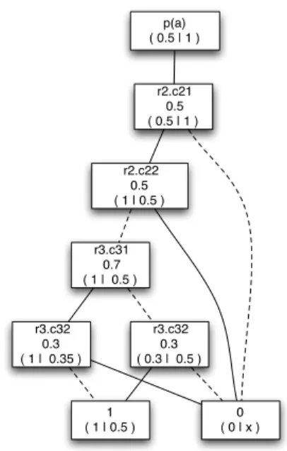
p(a) ( 0.5 | 1 ) r2.c21 0.5 ( 0.5 | 1 ) r2.c22 0.5 ( 1 | 0.5 ) r3.c31 0.7 ( 1 | 0.5 ) r3.c32 0.3 ( 1 | 0.35 ) r3.c32 0.3 ( 0.3 | 0.5 ) 0 ( 0 | x ) 1 ( 1 | 0.5 )

Fig. 2.BDD representing the formulaf given in Example 4. The root node indicates the ob-served interpretation. The terminal nodes represent whether the path starting at the root node yields this interpretation. The other nodes are annotated with the rulerand head elementcthey represent, in the form of the Boolean variabler.cused inf. If a node is left using a solid edge, the corresponding variable is assigned the value true, otherwise it is assigned the value false. Also given are upward probabilitiesα(N)and downward probabilitiesβ(N)for all nodesN, as

(α(N)|β(N)).

From the formulaf, areduced ordered binary decision diagram(BDD) [21] is con-structed. Let x1, . . . , xn denote an ordered set of Boolean variables (such as ther.c

contained inf). A BDD is a rooted, directed acyclic graph, in which nodes are anno-tated with variables and have out-degree2, indicating that the variable is either true or false. Furthermore, there are two terminal nodes labeled with0and1. Variables along any path from the root to one of the two terminals are ordered according to the given variable ordering. The graph compactly represents a Boolean functionfover variables

x1, . . . , xn: given an instantiation of thexi, we follow a path from the root to either1

or0 (indicating thatf is true or false). Furthermore, the graph must be reduced, that is, it must not be possible to merge or remove nodes without altering the represented function. More formally, a BDD graph is said to be reduced if no further reduction operations can be applied. Reduction operations are (1) to merge any two isomorphic subgraphs in the BDD structure, and (2) to remove any node whose two children are isomorphic. It can be shown that reduced ordered BDD structures are a unique repre-sentation for any Boolean function, given a fixed variable ordering (cf. [21] for more details). Figure 2 shows the BDD resulting from the formulaf given in Example 4.

From the BDD graph,P(It+1|I[0,t])can be computed in linear time using dynamic programming. The resulting algorithm is strongly related to the algorithm for inference

in ProbLog theories [17], and will now be described in detail. First note that there is a one-to-one correspondence between paths in the BDD from the root to the1-terminal and selections yieldingIt+1, where the path indicates which of the Boolean variables

r.cinf are assigned the value true, or equivalently, which head elementchas been selected for ruler. To see this, consider Step 3 of the algorithm for converting a given inference problem into the BDD. It ensures that exactly one head element is chosen for every rule. Thus, in the BDD representation, every path to the1-terminal must pass through all Boolean variables; otherwise, the state of one variable could be altered, violating the constraint encoded in Step 3 of the conversion algorithm.

We now recursively define for every nodeN in the BDD anupward probability α(N)as follows:

1. The upward probabilities for terminal nodes are defined as

α(0-terminal) = 0and α(1-terminal) = 1.

2. LetN be a node in the BDD representing the Boolean variabler.c, withra rule andcone of its head elements. LetN−_{, N}1_{denote the children ofN, withN}−_on

the negative andN+_{on the positive branch. Then}

α(N) =α(N−) +P(c|r)α(N+).

Furthermore, we recursively define adownward probabilityβ(N)as follows: 1. The downward probability of the root node is defined as

β(root) = 1. (5)

2. LetN be a non-root node in the BDD. LetN1, . . . , Nk denote the parents ofN,

withN1, . . . , Nl=pa+(N)reachingNby their positive branch andNl+1, . . . , Nk =

pa−(N)reachingN by their negative branch. Then

β(N) = l X i=1 β(Ni)P(ci |ri) + k X i=l+1 β(Ni) (6)

whereri.ciis the Boolean variable associated with nodeNi.

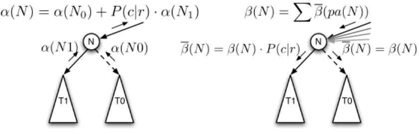
The definition of upward and downward probabilities is visualized in Figure 3. The valuesα(N)andβ(N)can be interpreted as probabilities of partial selections, which are determined by the path from the 1-terminal (α) or the root (β) to the node N. They roughly correspond to the forward-backward probabilities used for inference in hidden Markov models [3], or inside-outside probabilities used in stochastic context free grammars.

The following theorem states that the desired probabilityP(It+1|I[0,t])for infer-ence can be easily obtained given the upward and downward probabilities:

Theorem 2. Let Bbe a BDD resulting from the conversion of an inference problem P(It+1|I[0,t]), annotated with upward and downward probabilities as defined above,

and let

Γ ={σ|I[0,t]

σ

N T0 T1 α(N1) α(N0) α(N) =α(N0) +P(c|r)·α(N1) N T0 T1 β(N) =!β(pa(N)) β(N) =β(N)·P(c|r) β(N) =β(N)

Fig. 3.Calculation of upward and downward probabilities for internal nodes in the BDD.

be the set of selections yieldingIt+1. Then

α(root) =X

σ∈Γ

P(σ)

=P(It+1|I[0,t]). (7)

A proof of the theorem is given in Appendix A. Note that the downward proba-bilities will only be needed for the parameter estimation algorithm discussed in Sec-tion 3.4. Computing upward and downward probabilities from their recursive defini-tions is straightforward, thus Theorem 2 concludes the description of the BDD-based inference algorithm for CPT-L.

Computational costs are linear in the size of the BDD graph. The efficiency of this method thus crucially depends on the size of this graph, which in turn depends strongly on the chosen variable orderingx1, . . . , xn. Unfortunately, computing an optimal

vari-able ordering is NP-hard. However, existing implementations of BDD packages1

con-tain sophisticated heuristics to find a good ordering for a given function in polynomial time.

3.3 Partially Lifted Inference for CPT-Theories

We have so far specified CPT-L theories using first-order logic, but carried out in-ference at the ground level. This is a common strategy in many statistical relational learning frameworks: the first-order model specification serves as a template language from which a ground model is constructed for inference. A popular approach is to use graphical models as ground models. These can be directed (as in Relational Bayesian Networks [22], Bayesian Logic Programs [12], or CP-logic [11]), or undirected (as in Markov Logic Networks [10]).

In CPT-L, the grounded inference problem takes the form of a (propositional) Boolean formula, for which we need to compute all satisfying assignments. This prob-lem can be solved efficiently using binary decision diagrams, as shown in Section 3.2. However, the size of the inference problem (and resulting BDD) depends on the size of the grounded order model, which can be large compared to the original first-order model specification. Recent work on lifted inferencein first-order models (see,

for example, [23] and [24]) has shown that computational efficiency can be improved significantly if inference is performed directly at the first-order level. We now discuss a lifted inference algorithm for CPT-theories. The general idea is to solve a part of the overall inference problem directly at the first-order level, without compiling it into the binary decision diagram. The approach is best illustrated using an example:

Example 5. Reconsider the CPT-Theory given in Example 2. Suppose we want to compute the probability P(It+1 | I[0,t]), where It = {q(a), q(b), p(1), p(2), p(3)},

It+1={p(a), p(b)}, andI[0,t−1]are irrelevant as the theory refers only to the previous time-point. Rulesr1andr3are applicable, and

Rt={r1{X/a}, r1{X/b}, r3{X/1}, r3{X/2}, r3{X/3}}. We need to compute P(It+1|It) = X σ∈Γ P(σ) (8)

whereΓ is the set of selections yieldingIt+1fromIt. Computing this sum over

proba-bilities of selectionsσ∈Γ is the ground inference problem, which can be solved using BDDs as explained in Section 3.2. According to (1), theP(σ)are of the form

P(σ) =f11f12f31f32f33

wheref11, f12 ∈ {0.2,0.8}are the probabilities of selected head elements of ground rulesr1{X/a}, r1{X/b} ∈ Rt, andf31, f32, f33 ∈ {0.7,0.3}are the probabilities of selected head elements of ground rulesr3{X/a}, r3{X/b}, r3{X/c} ∈Rt.

However, inspecting ruler1 andIt+1, we see that irrespective of the substitution

θgrounding ruler1inIt, only the first head element ofr1 can be used in a selection. Thus, factorsf11andf12are always0.2, and (8) simplifies to

P(It+1|It) = 0.2·0.2 X

σ0_∈Γ0

P(σ0) (9)

whereσ0only selects head elements for ruler3. That is,P(σ0)is of the form

P(σ0) =f31f32f33.

Note that the remaining ground inference problem—summing over the partial selec-tions σ0_{—is smaller than the original one given by (8). The remaining problem can}

be solved using the BDD-based inference method as explained above. However, when converting this inference problem to a Boolean formulaf, we need to take into account that some facts appearing in the next interpretationIt+1 have already been generated by the head elements selected for groundings of ruler1, and thus do not need to be gen-erated anymore by groundings of ruler3. That is, we simply ignore already generated facts in Step 4 of the construction off.

In fact, we can go one step further, and note that also for ruler3we can determine the selected head element irrespective of the substitution used to ground the rule inIt. It

It+1given that the bodyp(X)is grounded inIt, thus only the second head element can

be used for any grounding of ruler3in any selectionσ0. Thus, Equation (9) is further simplified to

P(It+1|It) = 0.2·0.2·0.3·0.3·0.3

= 0.2Kr1_0.3Kr3 whereKriis the number of groundings of ruleriinIt.

The key observation in the above example is that for bothr1andr3we could log-ically infer the head element used in any selectionσ ∈Γ under any grounding of the rules inIt. Note that in general, only a subset of the rules can be removed from the

ground inference problem in this way.

Generalizing from Example 5, we can describe the partially lifted inference algorithm for any given CPT-theory T = {r1, . . . , rk} and inference problem

P(It+1|I[0,t])as follows:

1. LetRtdenote the set of all ground rules applicable inI[0,t] 2. Define

Rt={rθ∈Rt|It+1,I[0,t]logically determine the head element selected forrθ} For a rulerθ∈Rt, letσ(rθ)denote the head element that must be selected.

3. Compute P(It+1|I[0,t]) = Y rθ∈Rt P(σ(rθ)|rθ) X σ0_∈Γ0 P(σ0) = Y r∈T Y cr∈head(r) P(cr|r)Kr,c X σ0_∈Γ0 P(σ0), (10) where Kr,c=|{rθ∈Rt|σ(rθ) =cθ}|

andΓ0is the set of selections of head elements for rules inRt\Rtthat yieldIt+1 fromI[0,t], given that we select head elementσ(rθ)for rules inrθ ∈ Rt. Note

that in (10) we have integrated all ground rules for which a particular head element

crhas to be selected into one factor, which has to be taken to the power ofKr,c,

namely the number of such ground rules. Thus, we have performed a partially lifted probability calculation.

The setRtcontains those grounded rulesrθfor which we can prove — using logical

inference onbody(rθ),head(rθ), and the interpretationsI[0,t]andIt+1— that a partic-ular head elementσ(rθ)has to be selected forrθ. For instance, all groundings of ruler1 in Example 5 are in this set, because no ground facts of the formq(X)θappear inIt+1, and thus the first head element ofr1always has to be selected. In fact, for Example 5 we haveRt = Rt. The term Kr,c is the number of groundings of a ruler ∈ T for

which we know that the head elementc ∈ head(r)is selected for the grounded rule. For instance, in Example 5,Kr1,p(X) = 2andKr3,nil = 3. In practice, the counting

variablesKr,ccan be computed as follows. For each ruler, we first determine the set of

groundingsθsuch thatrθholds inI[0,t]and exactly one of the grounded head elements holds inIt+1; this can be achieved with a single logical query. We then count for each head elementcr∈head(r)the number of times the unique grounded head determined

in the first step was subsumed bycr, this yields the termKr,c.

Comparing the outlined partially lifted inference algorithm to other lifted inference algorithms proposed in the literature, such as first-order probabilistic inference [23] or lifted inference with counting formulas [24], we note that it is much simpler and, correspondingly, more limited in scope. Nevertheless, it proved surprisingly effective in our experimental evaluation (see Section 4).

Note that the efficiency of the presented inference algorithm depends on the fact that the selection of a particular head element is enforced by a given successor interpretation. This in turn depends on the closed-world assumption, which states that any atom not observed is false.

3.4 Parameter Estimation

Assume the structure of a CPT-theory is given, that is, a setT ={r1, . . . , rk}of rules of the form

ri= (ci1:pi1)∨. . .∨(cini :pini)←−bi1, . . . , bimi,

whereπ={pij}i,jare the unknown parameters to be estimated from a set of training

sequencesD. A standard approach is to find maximum-likelihood parameters

π∗= arg max

π P(D |π),

that is, to set the parameters such that we maximize the probability of generating the dataDfromT. When generatingDfromT, a ruleri∈Tis typically applied multiple

times: in the form of different groundingsriθ, and in different transitions (appearing in

different training sequences). We would like to set

∀i, j: pij =

κij

Pni

l=1κil

, (11)

whereκijdenotes the number of times head elementcijwas selected in any application

of the ruleriwhile generatingD. However, the quantityκijis not directly observable.

To see why this is so, first consider a single transitionI[0,t] → It+1 in one training sequence. We know the set of rulesRtapplied in the transition; however, there are in

general many possible selectionsσof rule head elements yieldingIt+1. The information about which selection was used, that is, which rule has generated which fact inIt+1, is hidden. We will now derive an efficient Expectation-Maximization algorithm in which the unobserved variables are the selections used at a transition, andκij the sufficient

statistics. To this aim, we first need to compute expected values of the κij given the

observations and the current model parameters π, and then re-estimate π according to (11) where theκijare replaced by their expectation.

To keep the notation uncluttered, we first consider a single transition

κθ

ij ∈ {0,1}denote whether the grounded head elementcijθwas selected in the

appli-cation of a grounded ruleriθ∈Rt. Let furthermoreΓ ={σ|I[0,t]

σ

→It+1}be the set of selections yieldingIt+1. For a given selectionσ∈Γ, we have

κθij = ( 1 : σ(riθ) =cijθ 0 : otherwise, (12) and κij = X θ:riθ∈Rt κθij (13)

where the sum runs over all groundingsriθ ∈Rtof ruleri. However, the selectionσ

is not observed, thus we instead have to consider the expectation_E[κij | π, ∆]ofκij

with respect to the posterior distributionP(σ|π, ∆)over selections given the data and current parameters. It holds that

E[κθij|π, ∆] =P(κ θ ij = 1|π, ∆) =X σ∈Γ P(κθij= 1|σ)P(σ|π, ∆) (14) whereP(κθ

ij = 1|σ)∈ {0,1}according to (12). Equation (13) now implies

E[κij|π, ∆] = X

θ:riθ∈Rt

E[κθij|π, ∆],

which concludes the expectation step of the Expectation-Maximization algorithm for a single transition ∆. If the dataDcontains multiple transitions (possibly appearing in multiple sequences), we can simply sum up the quantities_E[κij | π, ∆] for each

transition. Finally, given the expectation of the sufficient statisticsκij, the maximization

step in EM is

p(_ijnew)=_PE[κij |π,D]

jE[κij |π,D]

.

As usual, expectation and maximization steps are iterated until convergence in likeli-hood space.

The key algorithmic challenge in the outlined EM algorithm is to compute the ex-pectation given by (14) efficiently. Note that this again involves summing over all se-lections yielding the next interpretation, much as in the inference problem discussed in Sections 3.2 and 3.3. In fact, the quantityE[κθij | π, ∆]can also be obtained from

the upward and downward probabilities introduced in Section 3.2. More formally, the following holds:

Theorem 3. Letpij be the parameter associated with head elementcij in ruleri, let

∆ = I[0,t] → It+1 be a single transition, and letriθ ∈ Rtdenote a grounding of

Boolean variableriθ.cijθresulting from the grounded ruleriθ, and letNl+be the child

on the positive branch ofNl. Then

E[κθij|π, ∆] = 1 P(It+1|I[0,t]) k X l=1 β(Nl)pijα(Nl+). (15)

As for the inference problem discussed in Section 3.2, we can thus compute the estimation step given by (14) in time linear in the size of the BDD. The theorem can be proven using similar techniques as in the proof of Theorem 2; however, the proof is slightly more involved and thus moved to Appendix A.

Finally, note that at this point we can again make use of the partial lifted inference algorithm discussed in Section 3.3. A part of the expectation computation is then solved directly at the first-order level, while the rest is solved using dynamic programming in the BDD as explained above.

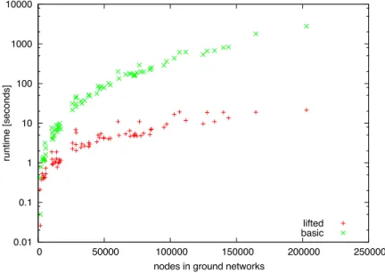
Note that the presented algorithms for inference and parameter estimation can be significantly more efficient than the corresponding algorithms in the more general CP-logic framework. Specifically, in CP-CP-logic the inference and learning problems basically have to be grounded into a Bayesian Network, which can grow very large depending on the characteristics of the domain. This often makes (exact) inference computationally challenging. In contrast, the inference and learning techniques we discussed here take advantage of the particular problem setting and model structure (that is, sequential and fully observable data). The experimental evaluation presented in Section 4 indeed shows that with these techniques we can perform exact inference in only seconds, for problems where the ground Bayesian Network would contain hundreds of thousands of nodes.

3.5 Prediction

Assume we are given an observation sequenceI0, . . . , It, a CPT-theoryT, and a

prop-erty of interest F (represented as a first-order query), and would like to compute

P(It+d|=F |I0, . . . , It,T). For instance, a robot might like to know the

probabil-ity that a certain world state is reached at timet+d, given its current world model and observation history. Or, in the MMOG domain, we might want to compute the probabil-ity that a particular player will have won the game at timet+d, given a model of game dynamics and an observation history. We will assume thatF is any first-order query that could be posed to a logic programming system such as Prolog, making use of the available background knowledgeB.

Powerful statistical relational learning systems are in principle able to compute the quantityP(It+d |= F | I0, . . . , It,T)exactly by “unrolling” the world model into a

large dynamic graphical model. However, this is computationally expensive as it re-quires to marginalize out all (unobserved) intermediate world statesIt+1, . . . , It+d−1, and thus often not practical in complex worlds. In contrast, inference in CPT-theories draws its efficiency from the full observability assumption, as outlined in Section 3. As an alternative to the “unrolling” approach, we thus propose a straightforward sample-based approximation to computeP(It+d |= F | It,T)that preserves the efficiency

variableIt+d |=F givenT andI0, . . . , It, and estimate the desired probability as the

fraction of positive samples.

GivenI0, . . . , It, it is straightforward to obtain independent samples of the

con-ditional distribution P(It+1, . . . , It+d | I0, . . . , It,T) by forward sampling from

the stochastic process represented by T, as explained in Section 3.1. Ignoring

It+1, . . . , It+d−1, we can simply check whetherIt+d |= F in the sampled

interpre-tation It+d. After repeatedly sampling interpretations I

(1)

t+d, . . . , I

(K)

t+d in this fashion,

the fraction ofI_t(₊k)_d for which I_t(₊k)_d |= F is then an unbiased estimator of the true probabilityP(It+d |=F | It,T), and will in fact quickly converge towards this true

probability for largeK.

4

Experimental Evaluation

In this section, we experimentally validate the proposed CPT-L approach in several (ar-tificial and real-world) domains as well as in different learning settings. The general set-ting discussed in this paper, namely construcset-ting models for stochastic processes with complex state representations, covers a wide range of application domains. It is appro-priate whenever systems evolve over time and are complex enough that their states can-not easily be described using a propositional representation. A prominent example are states that are characterized by a graph structure relating different agents and/or world artifacts at a given point in time (as in dynamic social networks, computer networks, the world wide web, games, marketplaces, et cetera). In this setting, observations consist of sequences of labeled (hyper)graphs, cf. Figure 8. To experimentally evaluate CPT-L, we have selected the following domains as representative examples:

Stochastic Blocks World Domain This domain is a stochastic version of the well-known artificial blocks world domain, representing an agent that is moving blocks which are stacked on a table. We use this artificial domain to perform controlled ex-periments, testing the scaling and convergence behavior of inference and learning algo-rithms.

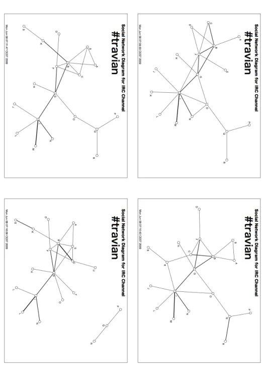
Chat Room DomainThis domain is concerned with the analysis of user interaction in chat rooms. We have monitored a number of IRC chat rooms in real time, and recorded who was sending messages to whom using the PieSpy utility [25]. This results in dy-namically changing graphs of user interaction, representing the social network structure among chat room participants, cf. Figure 5. We learn these dynamics using separate models for different chat rooms. The resulting set of models can be used to visual-ize commonalities and differences in the behavior displayed in different chat rooms, thereby characterizing the underlying user communities.

Massively Multiplayer Online Game Domain As a final evaluation domain intro-duced in [14], we consider the large-scale massively multiplayer online strategy game Travian3. Game worlds feature thousands of players, game artifacts such as cities, armies, and resources, and social player interaction in alliances. Game states in Travian

2

The implementation, models and data will be made available at http://www.ingothon.de/ 3_{www.travian.com;www.traviangames.com}

are complex and richly structured, and transitions between game states highly stochas-tic as they are determined by player actions. We have logged the state of a “live” game server over several months, recording high-level game states as visualized in Figure 8. We address different learning tasks in the Travian domain, such as predicting player ac-tions (prediction setting) and identifying groups of cooperating alliances (classification setting).

The goal of our experimental study is two-fold. First, we want to evaluate the effec-tiveness of the proposed approach. That is, we explore whether it is possible to learn dynamic stochastic models for the above-mentioned relational domains, and to solve the resulting inference, prediction, and classification tasks. Our second goal is to evaluate the efficiency of the proposed algorithms. That is, we will evaluate the scaling behavior for domains with a large number of objects and relationships, and in particular explore the advantage of performing partially lifted inference in such domains. Experiments to address these questions will be presented in turn for the three outlined evaluation domains in the rest of this section.

4.1 Experiments in the Stochastic Blocks World Domain

As an artificial testbed for CPT-L, we performed experiments in a stochastic version of the well-known blocks world domain. The domain was chosen because it is truly relational and also serves as a popular artificial world model in agent-based approaches such as planning and reinforcement learning. Moreover, application scenarios involving agents that act and learn in an environment are one of the main motivations for CPT-L. World Model The blocks world we consider consists of a table and a number of blocks. Every block rests on exactly one other block or the table, denoted by a facton(A, B). Blocks come in different sizes, denoted bysize of(A, N)withN ∈ {1, . . . ,4}. A predicatef ree(B)←−not(on(A, B))is defined in the background knowledge. Addi-tionally, a background predicatestack(A, S)defines that blockAis part of a stack of blocks, which is represented by its lowest blockS. Actions in the blocks world domain are of the formmove(A, B). If bothAandBare free, the action moves blockAonB

with probability1−, with probabilitythe world state does not change. Furthermore, a stackScan start to jiggle, represented byjiggle(S). A stack can start to jiggle if its top block is lifted, or a new block is added to it. Furthermore, stacks can start jiggling without interference from the agent, which is more likely if they contain many blocks and large blocks are stacked on top of smaller ones. Stacks that jiggle collapse in the next time step, and all their blocks fall on the table. Two example rules from this domain are

(jiggle(S) : 0.2)∨(nil: 0.8)←−move(A, B), stack(A, S) (jiggle(S) : 0.2)∨(nil: 0.8)←−move(A, B), stack(B, S),

they describe that stacks can start to jiggle if blocks are added to or taken from a stack. Furthermore, we assume the agent follows a simple policy that tries to build a large stack of blocks by repeatedly stacking the free block with second-lowest ID on the free block with lowest ID. This strategy would result in one large stack of blocks if stacks

-10000 -9000 -8000 -7000 -6000 -5000 -4000 -3000 -2000 -1000 0 2 4 6 8 10 Log-Likelihood

Iterations of the EM-Algorithm 10 blocks 25 blocks 50 blocks 0 2 4 6 8 10 12 10 20 30 40 50

runtime [minutes] for 10 iterations

Number of blocks runtime

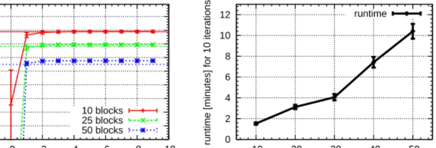
Fig. 4.Left graph: per-sequence log-likelihood on the training data as a function of the EM it-eration. Right graph: Running time of EM as a function of the number of blocks in the world model.

never collapsed. In our experiments, the policy was supplied as background knowledge, that is, the predicatemove/2was hard-coded by a logical definition in the background knowledge and not part of the learning problem. The model had14rules with24 pa-rameters in total.

Results in the Blocks-World Domain In a first experiment, we explore the conver-gence behavior of the EM algorithm for CPT-L. The world model together with the policy for the agent, that specifies which block to stack next, is implemented by a (gold-standard) CPT-theoryT, and a training set of20 sequences of length50 each is sampled fromT. From this data, the parameters are re-learned using EM. Figure 4, left graph, shows the convergence behavior of the algorithm on the training data for different numbers of blocks in the domain, averaged over15runs. It shows rapid and reliable convergence. Figure 4, right graph, shows the running time of EM as a func-tion of the number of blocks. The scaling behavior is roughly linear, indicating that the model scales well to reasonably large domains. Absolute running times are also low, with about 1minute for an EM iteration in a world with 50blocks4_{. This is in}

contrast to other, more expressive modeling techniques which typically scale badly to domains with many objects. The theory learned (Figure 4) is very close to the ground truth (”gold standard model”) from which training sequences were generated. On an independent test set (also sampled from the ground truth), log-likelihood for the gold standard model is -4510.7, for the learned model it is -4513.8, while for a theory with randomly initialized parameters it is -55999.4 (50 blocks setting). Manual inspection of the learned model also shows that parameter values are on average very close to those in the gold-standard model.

The experiments presented so far show that relational stochastic domains of sub-stantial size can be represented in CPT-L. The presented algorithms are efficient and scale well in the size of the domain, and show robust convergence behavior.

Fig .5. User interaction graphs from the Chat Room Domain. Sho wn are four dif ferent time points during the observ ation sequence recorded for the ir c.tr avian.or g chat room.

4.2 Experiments in the Chat Room Domain

For our experiments in the chat room domain, we have selected the following 7

well-frequented IRC chat rooms: [email protected], [email protected], [email protected], [email protected], [email protected], [email protected], and [email protected]. Each chat room was monitored for one day using the PieSpy utility [25], generating a sequence of user interaction graphs as those shown in Figure 5. For each chat room, we selected the first100observations in the sequence of user interaction graphs as a single observation sequence for that chat room, yielding

7observation sequencesS1, . . . , S7.

We have again hand-coded a simple CPT-theoryT for this domain, which makes use of a number of graph-theoretic properties defined in the background knowledge, such as graph centrality, node degree, closeness, betweenness, and co-citation. As an example rule, consider

communicates(P1, P2) : 0.1∨nil: 0.9←−cocitation(P1, P2, CC),

¬communicates(P1, P2),¬communicates(P2, P1)

encoding that two chat participants start talking to each other if there is a third partic-ipant with whom they have both talked before. The following three rules encode that a random person starts to communicate with another person which has above average

betweeness,degree, orcloseness.

communicates(P1, P2) : 0.1∨nil: 0.9←−betweeness(P1, C1), avg betweeness(Avg), C1> Avg,

¬communicates(P1, P2),¬communicates(P2, P1)). communicates(P1, P2) : 0.1∨nil: 0.9←−degree(P1, C1), person(P2),

avg degree(Avg), C1> Avg,

¬communicates(P1, P2),¬communicates(P2, P1). communicates(P1, P2) : 0.1∨nil: 0.9←−closeness(P1, C1), person(P2),

avg closeness(Avg), person(P1), C1> Avg,

¬communicates(P1, P2),¬communicates(P2, P1).

In the model definition rule heads also contain a third head element for reversed com-munication directioncommunicates(P2, P1), which was omitted above for increased readability. In total the model had7rules with11parameters (note that a rule with three head elements has two parameters, as parameters must sum to one).

For each chat room we learn the parameters of the CPT-theoryT using the EM al-gorithm presented in Section 3.4, resulting in7CPT-theoriesT1, . . . ,T7with the same rule structure but different parameters. Learning took about10seconds per theoryTi.

4

All experiments were run on standard PC hardware, 2.4GHz Intel Core 2 Duo processor, 1GB memory.

The learned CPT-theories can be seen as a probabilistic representation of the typical interaction behavior among members of that chat room, reflecting the corresponding different user communities. For instance, they could represent how quickly the interac-tion graph changes, the degree of connectivity in the interacinterac-tion graph, or how large the fluctuation in chat participants is over time. The goal of our experiment is to visualize the commonalities and differences in the behavior of these different user groups. To this end, we have evaluated the likelihoodP(Si| Tj)of each sequenceSiunder the learned

CPT-theoryTj. This gives an indication as to how well the behavior in chat roomiis explained by the model learned for chat roomj, thus indicating the similarity in user behavior for the corresponding two communities.

The result of this experiment is visualized in Figure 6. We can distinguish differ-ent clusters of chat rooms, or, equivaldiffer-ently, user communities. For instance, chat rooms that are concerned with recreational topics such as [email protected] [email protected] (as well as [email protected]) are clearly distinguishable from chat rooms concerned with more “serious” topics such as [email protected] and

[email protected]. Manual inspection of the learned rule parameters showed that in the “serious” chat domains the likelihood of a communication between two players mostly depends on the betweenness and degrees of the nodes involved, while in the “recreational” chats shared cocitations are more important.

travian football iphone computer poker math politics

travian football iphone computer

poker math _politics

Fig. 6.Plot of the likelihoodP(Si| Tj)of a sequenceSi(corresponding to chat roomi) under

the CPT-theoryTj(learned on chat room j). Rows correspond to models Tj and columns to

sequencesSi. Lighter colors indicate higher likelihoods.

4.3 Experiments in the Massively Multiplayer Online Game Domain

We now report on experiments inTraviandomain. In Travian, players are spread over several independentgame worlds, with approximately20.000–30.000players interact-ing in a sinteract-ingle world. Travian gameplay follows a classical strategy game setup. A game

border border border border Alliance 1 Alliance 2 Alliance 3 Alliance 4 Alliance 5 Alliance 6 Alliance 7 Alliance 9 Alliance 10 Alliance 11 P 1 733 885 857 948 690 628 637 667 593 P 2 1010 994 977 788 P 3 1021 857 1000 974 P 5 885 979 632 927 936 1032 P 6 1032 1022 675 670 707 P 7 974 855 818 921 920 926 818 990 778 837 680 844 721 613 P 8 968 942 961 963 P 12 1000 1005 850 P 14 792 685 643 707 P 15 883 958 740 947 P 16 985 717 P 17 986 911 978 818 P 18 943 910 924929 947 1001 869 892 P 19 1045 1005 959 740 799 817 P 21 737 766 912 931 P 22 813 771 878 623 P 24 935 898 634 882 823 581 832 P 26 753 P 28 908 P 30 932 841 P 33 853 803 P 34 1018 797 P 36 904 1003 10281036 972976 982 920 823 783 717 P 37 1017 911 879 751 P 38 693 817 P 40 690 626 P 41 905 947 759 P 42 756 606 P 43 762 863 P 45 695 P 46 1001 833 P 47 991 833 638 P 50 882 857 864 P 51 951 1023 735 873 P 52 863 720 651 649 P 55 635 596 P 56 1042 1047 802 978 1043 984 P 57 996 936 928 924 1030 819 934 1007 996 1004 842 P 59 640 901 529 P 61 994 702 801 600 837 P 63 959 1031 811 P 64 934907 835 863 P 66 888 847 934 871 776 671 577 P 67 538 430 P 68 651 626 585 P 70 934823 940 795 P 72 782 664 P 74 808 790 999 835 927 744683 P 75 1083 961 794 1000 P 76 973 768 P 77 904 994 657 P 78 947 529 P 79 800 583 P 81 1017 978 928 820 1028 1044 870 1045 916 732 900 801 P 82 764 P 83 748 P 84 780 P 85 546 548 P 86 748 713 768 P 88 849 793 730 692 P 89 834 576 P 91 1035 836 P 92 488 P 95 744 966 937 961 P 97 931 P 98 990 P 99 880 P 100 8231000 794 P 101 854 810 765 P 105 904 831 736 830 786 P 106 752 P 107 730 P 111 977 991 823 440 736 614489 P 116 1002 986 550 P 120 880 933 940 867 768743 P 121 1049 1013 968 986 942 748 P 122 1060 908886 973 783 P 123 799 P 124 9891060 926 920 P 125 812 858 913 620 P 126 1190 849 612 803 799 P 127 776 892 825 833 607 P 128 899 P 129 634 1001 650 P 132 736 546 436 P 134 744 880 P 135 948 825 P 136 720 839 952 807 P 137 665 850 677 863 751 756 761 674 P 138 985 728 789 724 932 P 139 960590 P 140 954 944 1020 996 986 770 P 141 859 892 526 P 142 967 P 143 1040 1055 P 145 693 P 146 1106 1068 P 150 1005 773 793 P 153 919 969 783 905 991 954 946 910 884804 594 P 154 892855 P 156 943 P 157 863742641 P 158 897 P 159 920 P 167 843 712 798 790 739635 P 168 913 P 172 834 588 591 696 970 P 174 483 541 607 P 176 581 P 177 639 742719 P 179 717 882 842 542 P 180 958 999 P 181 1000 1035 985 1035 1060 1063 598 576 997 1003 P 183 896 852 699 P 185 937 936 958 812 P 186 973 895 P 187 911 P 189 1001 722 874 974 786 986 1014 780 P 191 888 830 P 193 718 P 195 753 P 199 966 950 P 201 713 606 P 202 905 953 861 952 872 848 703 801 784 898 832 805 P 203 761 775 P 205 854 892 509 899 867 700 643 P 212 921 517 688 690 560 577 P 213 613 P 217 985 953 1068 969 1008 1060 894 P 220 918 902 738 P 221 794 864 780 692 612 579 P 222 875 773 P 223 774 P 224 901791 477 P 228 667 583 630 P 230 818 P 231 793 879 826 705 P 233 746 P 234 747 P 235 972 889 788 P 236 1228 579 784 578 614 P 238 505 P 239 946 903 1030 976 925 799 865 P 240 1046 1055 1059 1029 1005 916 814 P 242 1066 891 928 1056 880 9231029 797 884 1059 1034 939 992 831 773 915 955 740 904 P 244 705 685 770 679 P 246 757 775 759 921 839

Fig. 7.High-level view of a (partial) game world in Travian. Circular nodes indicate cities, shown in their true positions on the game’s grid-map. Diamond-shaped nodes indicate players, and are connected to all cities currently owned by the player. Rectangular nodes indicate alliances, and are connected to all players currently members of the alliance. (The alliance affiliation is additionally indicated by color-coding of the cities and players.)

world consists of a largegrid-map, and each player starts with a singlecitylocated on a particular tile of the map. During the course of the game, players harvestresources

from the environment, improve their cities by construction ofbuildingsor research of

technologies, or found new cities on other (free) tiles of the map. Additionally, players can build different military units which can be used to attack and conquer other cities on the map, or trade resources on a global marketplace.

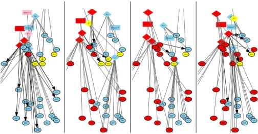
In addition to these low-level gameplay elements, there are high-level aspects of gameplay involving multiple players, which need to cooperate and coordinate their playing to achieve otherwise unattainable game goals. More specifically, in Travian players dynamically organize themselves intoalliances, for the purpose of jointly at-tacking and defending, trading resources or giving advice to inexperienced players. Such alliances constitute social networks for the players involved, where diplomacy is used to settle conflicts of interests and players compete for an influential role in the alliance. In the following, we will take a high-level view of the game and focus on modeling player interaction and cooperation in alliances rather than low-level game el-ements such as resources, troops and buildings. Figure 7 shows such a high-level view of a (partial) Travian game world, represented as a graph structure relating cities, play-ers and alliances which we will refer to as agame graph. It shows that players in one alliance are typically concentrated in one area of the map—traveling over the map takes time, and thus there is little interaction between players far away from each other.

We are interested in thedynamicaspect of this world: as players are acting in the game environment (e.g. by conquering other players’ cities and joining or leaving al-liances), the game graph will continuously change, and thereby reflect changes in the

border border border border Alliance 1 Alliance 2 Alliance 3 Alliance 5 P 2 1081 895 1090 1090 1093 1084 1090 915 1081 1040 770 1077 955 1073 804 1054 830 942 1087 786 621 P 3 744 748 559 P 5 861 P 6 950 644 985 932 837 871 777 P 7 946 878 864 913 P 9 border border border border Alliance 1 Alliance 3 Alliance 5 P 2 918 1090 931 779 977 835 781 958 1087 808 701 P 3 838 947 1026 1081 833 1002 987 827 994 663 P 5 1032 1026 1024 1049 905 926 P 6 986 712 985 920 877 807 P 7 895 959 P 10 824 border border border border Alliance 1 Alliance 3 Alliance 5 P 2 923 1090 941 784 983 844 786 966 1087 815 711 P 3 864 986 842 1032 1083 868 712 1002 1000 858 996 696 P 5 1039 1037 1030 1053 826 933 P 6 985 807 P 7 894 963 P 10 829 781 828 border border border border Alliance 1 Alliance 3 Alliance 5 P 2 938 1090 949 785 987 849 789 976 1087 821 724 P 3 888 863 868 1040 1083 896 667 1005 994 883 1002 742 P 5 1046 1046 1040 985 894 1058 879 938 921 807 P 6 P 7 P 10 830 782 829

Fig. 8.Travian game dynamics visualized as changes in the game graph (fort= 1,2,3,4,5). Bold arrows indicate conquest attacks by a player on a particular city.

social network structure of the game. As an example for such transition dynamics, con-sider the sequence of game graphs shown in Figure 8. Here, three players from the red alliance launch a concerted attack against territory currently held by the blue and yellow alliances, and partially conquer it.

Data Collection and Preprocessing The data used in the experiments was collected from a “live” Travian server with approximately25.000active players. Over a period of three months (December 2007, January 2008, February 2008), high-level data about the current state of the game world was collected once every24hours. This included information about all cities, players, and the alliance structure in the game. For cities, their size and position on the map are available; for players, the list of cities they own; and for alliances the list of players currently affiliated with that alliance.

The game data was represented using predicates city(C, X, Y, S, P) (city C of size S at coordinates X, Y held by player P), allied(P, A) (player P is a mem-ber of allianceA), conq(P, C)(indicating a conquest attack of playerP on cityC) andalliance change(P, A)(playerP changes affiliation to allianceA). A predicate

distance(C1, C2, D) with D ∈ {near, medium, f ar} computing the (discretized) distance between cities was defined in the background knowledge. Sequences consist of between29and31such state descriptions.

Classification Experiments As a classification setting, we consider the problem of identifying so-called meta-alliances in Travian, which was recently introduced by Karwath et al. [26]. A meta-alliance is a group of alliances that closely cooperate, thereby allowing large groups of players to work together. We manually identified meta-alliances in the collected game data based on the alliance names (a small free-text field).

For instance, it is easy to recognize that the alliances’.˜A˜.’,’.=A=.’, and’.-A-.’are dif-ferent wings of the same meta-alliance.

From all available game data,30sequences of local game world states were ex-tracted. Each sequence tracks a small set of players from three different alliances, two of which belong to the same meta-alliance (indicated by a factmeta alliance(a1, a2)). On average, sequences consist of25.8interpretations, every interpretation contains16.4

cities and10.6 players, and there are17.6conquest events per sequence. The30 ex-tracted sequences constitute positive examples. A further 60negative examples were obtained by giving the wrong meta-alliance information (i.e.,meta alliance(a1, a3)

ormeta alliance(a2, a3)).

We hand-coded a simple CPT-theory that encodes a few basic features that one would assume to be useful in such a task, such as whether two players in different al-liances a1 anda2 attack each other (indicating¬meta alliance(a1, a2)), or jointly attack a player from a third alliance (indicatingmeta alliance(a1, a2)). As an exam-ple, consider the following rule:

conq(C, P1) : 0.0061∨nil: 0.9939 ←−city(C, , , P2), player(P2, , A1), player(P1, , A2),¬meta alliance(A1, A2).

which states that the playerP1attacks a cityCof a playerP2who is not his alliance partner.

Such a CPT-theory can be used for classification as follows. Given a set of training sequencesD, we first split this set into positive sequencesD+and negative sequences

D−. We then learn the parameters of two CPT-theoriesT+andT−on the setsD+and

D−according to maximum likelihood using the EM algorithm presented in Section 3.4.

Note thatT+andT−both employ the simple rule set outlined above, and only differ in

their parameter values. Given a new test sequenceS, we then evaluate the likelihood of

S under the positive and negative models,P(S | T+)andP(S | T−), and predict the

class for which this likelihood is higher.

To evaluate the accuracy of CPT-L in the meta alliance classification task, we per-formed a10-fold cross-validation, using the same folds as used in [26]. Figure 9 com-pares the results obtained for CPT-L with those of the BOOSTEDREALsystem. BOOST

-EDREALis a state-of-the-art system for classification of (relational) sequences by align-ment, which uses a discriminative approach based on boosting the reward model used in the alignment algorithm [26]. Note that BOOSTEDREAL, in contrast to CPT-L, is not a generative model for sequences of interpretations, but rather a discriminative approach specifically tailored to classification problems. It is also significantly more complex, and the resulting models are harder to interpret, as the boosted reward function is rep-resented as an ensemble of relational regression trees. Figure 9 shows that CPT-L, at

82.22% with standard deviation of9.37, achieves a slightly lower accuracy than the best observed result for BOOSTEDREAL, although the difference is not significant as-suming equal variances for CPT-L and BOOSTEDREAL. Overall, we can conclude from this experiment that even with the simple rule set used, CPT-L is able to learn a model that captures useful information about the positive and negative class, and achieves similar accuracies as other state-of-the-art sequence classification schemes. Learning a