Modelling Tools and Simulation Platforms for Advanced Driver Assistance Systems

U

NIVERSITY OF

N

APLES

F

EDERICO

II

D

OCTORAL

S

CHOOL IN

C

IVIL

E

NGINEERING

P

D

P

H

S

,

T

U

D

E

D

T

Modelling Tools and Simulation Platforms for Advanced Driver

Assistance Systems

Maria Russo Spena

Tutor: Ph.D. Coordinator:

Prof. Eng. Gennaro Nicola Bifulco Prof. Arch. Elvira Petroncelli

Examiner:

‘Never argue with an idiot. It drags you to his level and beat you with the experience’ (cit. O. Wilde)

Overview

Recent developments in Advanced Driver Assistance Systems (ADAS) lead to the concept of eco-driving support systems, which assist drivers in controlling vehicles in a sustainable way by reducing fuel consumption and carbon dioxide emissions. In this thesis, an algorithm for an ecological Adaptive Cruise Control (ecoACC) system is designated. In order to test the system in MIL (Model in the Loop) and DIL (Driver In the Loop) environments, an important task is the specification of a fuel consumption model.

In the first part of the thesis an overview is presented about fuel consumption models and several eco-devices developed by different authors. In the second part an experimental campaign (with a sample of 100 drivers) is carried out in order to specify and to validate the model. The survey is supported by the DRIVEIN2 (DRIVEr monitoring: technologies, methodologies, and IN-Vehicle Innovative systems) project. As the major data are collected using the OBD-II port, and in particular the data related the instantaneous fuel consumption, a validation of the former data is carried out in collaboration with the CNR (Consiglio Nazionale delle Ricerche – Istituto motori).

To carry out a more realistic simulation a vehicle dynamics model was coupled with the ADAS model. The purpose of the implemented vehicle dynamics model is to simulate, in real time, the vehicle’s dynamic behaviour, thanks to continuous integration of the balance equations regulating the longitudinal and lateral vehicle motion. Furthermore, a model able to provide an estimation of real-time fuel consumption of the vehicle is developed: such a model is embedded in the vehicle model discussed in the following, in order to optimize consumption performance during driving task.

Index of Figures

Figure 1-Total model diagram proposed by Van der Voort et al. (2001) ... 11

Figure 2 – CompactDAQ and pc controller ... 15

Figure 3 – TRW Autocruise AC20 radar mounted behind, Xsense MTi-G ... 16

Figure 4 – Front and rear cameras ... 17

Figure 5 – OBD II port locates under the dashboard ... 18

Figure 6 –Instrumented Vehicle equipped with PEMS ... 19

Figure 7 – Diagram of power supply system of SEMTECH ... 20

Figure 8 – Scheme of devices mounted during the on-road test ... 21

Figure 9 – DICEA Driving simulator ... 21

Figure 10 – The experimental path ... 26

Figure 11 – The experimental path ... 29

Figure 12 – Percentage differences between aggregate data collected by the OBD port and by the PEMS for each driver. ... 39

Figure 13 – Empirical cumulative mass functions (ecmf) of gap between data collected by the OBD port and by the PEMS for Driver 6 (on the top) and Driver 3 (on the bottom) using different time slots. ... 41

Figure 14 – Empirical probability mass function (epmf) for aggregate data each 3 minutes differentiating for the median value of RPM ... 42

Figure 15 - Dependence of fuel metering on: (lefts side) Gas Pedal; (right side) Intake Air ... 45

Figure 16- Screenshot of the results for the null model (36) ... 46

Figure 17 – Box whisker plot of Fuel metering vs subjects ... 47

Figure 18 – Histogram of marginal residuals ... 54

Figure 20 – Empirical probabibilty mass function (epmf) and empirical cumulative mass function (ecmf) vs the percentage error

(ERRinst) of the two sub-samples ... 57

Figure 21 – Empirical probability mass function (epmf) and empirical cumulative mass function (ecmf) of the aggregate error (ERRaggr) for the calibration and the control sub-samples. ... 59

Figure 22 – Scheme of eco-drive system ... 61

Figure 23 – Architcture implemented in Matlab/Simulink ... 62

Figure 24 – ‘Simulated Driver’ sub-system ... 64

Figure 25 – Screenshot showing the vehicle dynamics Simulink model ... 66

Figure 26 – “Input/Output” Simulink subsystem ... 67

Figure 27 – “Control Unit Simulink subsystem” ... 67

Figure 28 – “Tires” Simulink subsystem ... 68

Figure 29 - “Vehicle Dynamics” Simulink subsystem ... 69

Figure 30 – “Gearbox Control Unit” Simulink subsystem ... 69

Figure 31 – Architecture implemented in DIL environment ... 71

Figure 32 – Simulink/SCANeR communication protocol ... 72

Figure 33 – SCANeR Studio window ... 73

Figure 34 - SCANeR Studio main ... 75

Figure 35 – (on the top) Leaves used for driver feedback, (on the bottom) Screenshot of graphical interface provides to driver ... 76

Index of Table

Table 1 – The sample ... 24

Table 2 - Correlation matrix ... 45

Table 3- Parameters of lme model (41) ... 48

Table 4 – Standardized beta for model (41) ... 49

Table 5 – Parameters of lme model (42) ... 50

Table 6 – Standardized beta for model (42) ... 50

Table 7 - LogLikelihood Ratio test for lme models (41) - (42) ... 51

Table 8 – Variance-Covariance matrix of random effects for lme model (42).. 51

Table 9 - LogLikelihood Ratio test for lme models (43) - (42) ... 52

Table 10 – Parameters of lme model (46) ... 55

Table 11 - Variance-Covariance matrix of random effects for lme model (46) 56 Table 12 – RMSE and MAPE computed for the two sub-samples ... 58

Table of contents

Chapter I – State of the art ... 4

1.1 Beyond the state of the art ... 13

Chapter II - Strategies and tools ... 14

Introduction ... 14

2.1 Tools ... 14

2.1.1 Instrumented Vehicle ... 14

2.1.2 Portable Emission Measurement System ... 18

2.1.3 Twins Driving Simulators ... 21

2.2 Experimental surveys and data collection ... 23

2.2.1 DriveIn2 experiment ... 23

2.2.2 DriveIn2 experiment add-on ... 28

Chapter III – Fuel consumption model ... 30

Introduction ... 30

3.1 Linear mixed effect model ... 30

3.1.1 Specification for all data ... 33

3.1.2 Maximum-Likelihood Estimation ... 34

3.2 Validation of OBD fuel consumption ... 37

3.3 Specification of fuel consumption model ... 42

Chapter IV – Implementation of ADAS in MIL and DIL environment ... 60

Introduction ... 60

4.1 The implemented model in MIL ... 60

4.2 The implemented model in DIL ... 70

Conclusion ... 77

Introduction

The research here presented takes place in the frame of driving behaviour studies, and the design of Advanced Driving Assistance Systems (ADASs). ADASs are developed using electronic control units (ECUs) that are aimed to supervise the safety, the comfort and/or the efficiency of the driving.

Their design is carried out by using the so-called automotive V-Cycle, a process of analysis, development and prototyping that envisages a first phase of conception of the control logic characteristics and mechanisms, a second phase in which the software needed to manage such a logic is developed, and a third phase consisting on the implementation of the ECU and the evaluation of its interaction with the other components (hardware sensors, actuators and other devices, control units) of the vehicle.

The first stage is called Model In the Loop (MIL), the model of the control logic interacts with the models (already certified and tested) that represent the operation of the entire vehicle (as well as the environment and traffic).

In the second phase, called Software In the Loop (SIL), the controller management software that implements the control logic interacts with other software codes and other system component models in a simulated

environment; however, the input and output of the tested software are of the same kind and type of real ones.

In the third stage, known as Hardware In the Loop (HIL), a prototype controller is actually developed (by using embedded programming techniques), and the obtained hardware-component is plugged into a mixed testing environment composed by both hardware and other software components (already developed and certified). The actual hardware/software mix depends on the particular aim of the experiment and is aimed at fully reconstructing the vehicle architecture.

The research here described falls in the MIL context and is aimed at enhancing existing ADAS testing platforms (generally developed in Matlab/Simulink) with the possibility of including more sophisticated models that takes into account the interaction of the controlled vehicle with other vehicles (traffic), and with the drivers’ behaviours. Particular focus is dedicated, in the previous framework, to the development of a fuel consumption module. It will be verified the possibility of including at the MIL level also observation of drivers’ reactions in a virtual environment (using Driving Simulators), thus creating a DIL (Driver In the Loop) level.

The choice of ADAS aimed to reduce fuel consumption and greenhouses gas emission, adopting an eco-driving style, is due to the fact that the fuel saving is a sensible topic. In fact, on 24 June 2013, the Environment Committee of the European Parliament approved an agreement on new rules to reduce the CO2 emissions of passenger cars. According to the text by 2021, for new vehicles sold in the EU, CO2 emissions must be reduced by 28% (from the current 132 g/Km to 95 g/Km). The text was approved by the plenary in Strasbourg on 24-27 February 2014. A possible approach to the problem is to act at the vehicle level, understanding what mostly affects fuel consumption, and developing the design of Advanced Driver Assistance Systems (ADASs) that help the drivers in adopting an eco-driving style.

The thesis is organized as follows: section 1 resumes the literature with respect to the various approaches used for the analysis of fuel consumption and

different eco-drive tools implemented and tested in real and virtual environment; in section 2 the two experiments, the tools adopted and the collected data are presented; in section 3 validation of OBD fuel data and characterization of fuel model are discussed, in section 4, implementation of eco-drive architecture in MIL and DIL are presented; and finally, some conclusions are drawn.

Chapter I

–

State of the art

Transport systems are affected by serious negative externalities in terms of both pollution (Davitashvili, 2009) and noise (Pamanikabud, 2009). Indeed it has been estimated that the impact of the transport sector is in the range of 20%–40% in terms of consumption of fossil fuels and emission of greenhouse gases and particulate (Cartenì, 2014). To manage and reduce these negative impacts, many fuel-consumption and air-pollution control policies have been adopted, such as the introduction of carbon-based vehicle tax systems (Chi, Guo, Zheng, & Zhang, 2014), incentives for the adoption of hybrid electric vehicle (Zhang, Xie, Rao, & Liang, 2014), improvements in vehicle technologies (catalytic converter, alternative fuels, engine efficiency), congestion charging, and incentives for using public transport. Furthermore it’s also important to pay attention on the effect of traffic calming measures on the environmental and energy impacts. These involve strategic measures to improve safety and enhance quality of life by reducing vehicle speed and/or cut-through volumes on streets or street networks. In fact as shown in the case study presented by Ahn et al. (2009), while traffic-calming measures reduce vehicle speed on neighbourhood streets enhancing road safety, these measures can result in significantly higher fuel consumption and emission rates when drivers accelerate aggressively.

A different effective and promising technique to increase fuel saving is eco-driving, which is essentially based on observing and controlling the driver behaviour. Eco-driving is defined as a decision-making process, which will influence fuel-savings and emissions intensity of a vehicle to reduce its environmental impact (Sivak & Schoettle, 2012).

At the transportation network level, eco-driving acts by implementing proper instruments for the evaluation and implementation of strategies for the reduction of traffic congestion [ (D'Acierno, Montella, & Gallo, 2011), (Gori, La Spada, Mannini, & Nigro, 2014)] and for optimum route choice in order to

limit CO2 emission and fuel consumption (eco-route, (Sivak & Schoettle,

2012)). Eco-driving at the single vehicle/driver level can be achieved through an understanding what primarily affects fuel consumption, and by developing ADASs that help drivers in adopting efficient driving styles in terms of emissions and energy consumption. At both levels, the effects of the adopted solutions can be investigated by using microscopic simulation tools, which allow the simulation of the interaction of vehicles in a traffic stream and the resulting kinematics (and dynamics) of the vehicles. Microscopic models make it possible to explicitly take into account different driving behaviours (Mauro, Giuffrè, Grana, & Chiappone, 2014) and engine characteristics [ (Donateo, 2013), (De Luca, Di Pace, & Marano, 2015)].

In the case of ADAS oriented to eco-driving, a model able to predict fuel consumption is a pre-requisite. Fuel consumption models can be implemented by following three different approaches: macro models, meso models and micro models. Macro models are able to predict fuel consumption for a relatively large region and for rather long periods of time; of course, for the purposes of this research they will not be processed. Meso models are based on average parameters (e.g., the average speed of the vehicle), and can be divided into two major categories: models based on correction factors [ (Ntziachristos, Gkatzoflias, Kouridis, & Samaras, 2009), (Brzezinski & Newell, 1998)], and models based on vehicle specific power (VSP) which is the power exerted per unit mass [ (Koupal, Cumberworth, Michaels, Beardsley, & Brzezinski), (Hui, Zhang, Yao, & Wang, 2007)]. Consumption calculated using these approaches reflects the average consumption for a certain class of vehicles, often presenting some deviance in results when considering a specific vehicle (Zhou, Huang, Weifeng, & Li, 2013).

This thesis focuses on the microscopic approach, in which developed models can be classified according to different criteria. First and foremost is the fuel supply—gasoline, diesel and newly developed hybrid vehicles. Second is the basis of the models. Some of them have as a basic principle the traction-law. These models estimate the fuel consumption as a function of the mass of the vehicle, the aerodynamic drag coefficient, the vehicle frontal area, the

vehicle acceleration and speed, the road gradient, etcetera. In particular, Post et al. (1984) developed a fuel consumption model that is a linear function of the instantaneous power demand; the model was built starting from the available data of chassis dynamometer experiments of 177 in-use vehicle. This model was subsequently enhanced in later publications [ (Akcelik, 1989), (Leung & Williams, 2000)]. In other cases, fuel consumption has been indirectly inferred from exhaust gas emissions, even in real time, using the carbon balance method (e.g., Rakha et al. (2004)). An important category concerns models based on laboratory-tests performed on a chassis dynamometer, that implements standard driving cycles such as the European NEDC (New European Driving Cycle), and the U.S. FTP (Federal Test Procedure) [ (Wong, 2001), (Rakha, Ahn, Moran, Searens, & Van den Bulck, 2011)].

For the scope of this thesis, it is worth pointing out approaches that make it possible to compute instantaneous fuel consumption, possibly at real-time. Moreover, these models are required for vehicle-specific application, thus it can be applied and specified for a each given vehicle it is applied to, without the need to be representative of the dispersion among several vehicles. For instance, Ahn (1998) developed a nonlinear regression model, in order to predict fuel consumption, as a polynomial combination of the instantaneous speed and acceleration, using different regression coefficients in the deceleration or acceleration phase, as shown in equation (1), in order to construct a dual-regime model. The model was calibrated using data collected at the ORNL (Oak Ridge National Laboratory) using a chassis dynamometer, data gathered using an on-board emission measurement device, and also data gathered by EPA (Environmental Protection Agency). This model differs from the others because, while these last were developed as power-demand models, the VT-Micro model was developed as a statistical model.

𝐹(𝑡) = { exp⁡(∑ ∑ 𝐿𝑖𝑗⁡𝑣(𝑡)𝑖 3 𝑗=1 3 𝑖=1 𝑎(𝑡) 𝑗_{) ⁡⁡𝑎(𝑡) ≥ 0} exp⁡(∑ ∑3 𝑀_𝑖𝑗⁡𝑣(𝑡)𝑖 𝑗=1 3 𝑖=1 𝑎(𝑡) 𝑗_{) ⁡⁡𝑎(𝑡) < 0} (1

Where Lij and Mij are model parameters at speed exponent i and acceleration j, v(t) is the instantaneous vehicle speed at instant t expressed in kilometers per hour; and a(t) is the instantaneous vehicle acceleration (km/h/s).

In the same period, the University of California (Barth, et al., 2000) presented the Comprehensive Modal Emissions Model (CMEM) which is able to predict instantaneous fuel consumption and emissions in three different driving cycles for both light and heavy vehicles; the model uses as input variables the vehicle kinematic (acceleration, velocity, etc.), the characteristics of the road (e.g., slope), and motor data (such as the coefficient of cold starting, and the coefficient of engine friction), as shown in (2) - (5) :

𝐹𝑅 [𝑔 𝑠] = (𝐾 ∙ 𝑁 ∙ 𝑉 + 𝑃 𝜂)⁡ 1 43.2⁡(1 + 𝑏1⁡(𝑁 − 𝑁𝑂)2) (2 Where FR is fuel rate grams/second, P is engine power output in kW (eq. (4a)), K is the engine friction factor (described in eq. (3)), N is engine speed (revolutions per second), N0 is the idling engine speed (eq. (5)), V is engine displacement (liter), and η≈0.45 is a measure of indicated efficiency for diesel engine. C≈0.00125 and b1≈10-4 are coefficients; 43.2 kJ/g is the lower heating value of a typical diesel fuel. In particular:

𝑃[𝑘𝑊] =𝑃𝑡𝑟𝑎𝑐𝑡 𝜀 +⁡𝑃𝑎𝑐𝑐 (4a 𝑃_{𝑡𝑟𝑎𝑐𝑡}[𝑘𝑊] = 𝐴⁡𝑣 + 𝐵⁡𝑣 + 𝐶⁡𝑣 + 𝑀⁡(0.447𝑎 + 𝑔 sin(𝜃))𝑣⁡0.447 1000 (4b 𝑁0 = 30⁡√ 3.0 𝑉 (5

Where K0 is constant engine friction factor that varies depending on the vehicle. Ptract e Pacc are respectively the total tractive power requirements and the engine power demand associated with the operation of vehicle accessories such as air conditioning usage; ε is vehicle drivetrain efficiency. In particular the total tractive power requirements, Ptract, placed on the vehicle (at the wheels) is described in eq, (4b), where M is the vehicle mass with appropriate inertial correction for rotating and reciprocating parts (kg), v is speed (mph), a is acceleration (mph/s2), g is the gravitational constant (9.81 m/s2), and θ is the road grade angle in degrees. The coefficients A, B and C involve rolling resistance, speed-correction t rolling resistance, and air drag factors.

Moreover all models presented in the literature produce a bang-bang type of control system (i.e. optimal control entails full-throttle input and full braking input); to overcome this type of problem, Rakha et al. (2011) developed the Virginia Tech Comprehensive Power- based Fuel consumption Model (VT-CPFM). In fact a model that results in a bang-bang control system would indicate that the optimum fuel economy control would be to accelerate at full throttle in order to reduce the acceleration time. This type of control, which is obviously incorrect, would induce the driver to drive as aggressively as possible in order to minimize her/his fuel savings. This is due to the fact that the partial derivative of fuel consumption rate (F) with respect to the engine torque (T) isn’t a function of engine torque, or 𝛿𝐹⁄_𝛿𝑇 ≠ ⁡𝑓(𝑇) (Saerens, Diehl, & Van den Bulck, 2010). As shown below eq. (6) the model is a second order polynomial as a function of the instantaneous vehicle power P(t):

𝐹(𝑡) = {𝛼0⁡+⁡𝛼1𝑃(𝑡)⁡+ 𝛼2𝑃(𝑡)2⁡⁡𝑃(𝑡) ≥ 0

⁡𝛼0⁡⁡⁡⁡⁡⁡⁡⁡⁡⁡⁡⁡⁡⁡⁡⁡⁡⁡⁡⁡⁡⁡⁡⁡⁡⁡⁡⁡⁡⁡⁡⁡⁡⁡⁡⁡⁡⁡⁡⁡⁡⁡𝑃(𝑡) < 0 (6 Here 𝛼0, 𝛼1⁡and 𝛼2 are the model parameters and P(t) is the instantaneous total power exerted by the vehicle at any instant t (kw), computed as:

𝑃(𝑡) = ⁡ (𝑅(𝑡) + 1.04⁡𝑚⁡𝑎(𝑡)

3600⁡𝜂𝑑 ) ⁡𝑣(𝑡) (7

With m corresponds to vehicle mass (kg), a(t) and v(t) are respectively the instantaneous acceleration and velocity at instant t, 𝜂_𝑑 is the driveline efficiency and R(t) is the resistance force given by the following equation:

𝑅(𝑡) = 𝜌

25.91𝐶𝑑𝐶ℎ𝐴𝑓𝑣2(𝑡) + 𝑚𝑔 𝑐𝑟0

1000(𝑐𝑟1⁡𝑣(𝑡) + 𝑐𝑟2⁡)

+ 𝑚𝑔𝐺(𝑡) (8

Equation (8) computes the sum of the aerodynamic, rolling and grade resistance forces acting on the vehicle. The parameters presented in that equations are: air density a level sea and a temperature of 15°C (𝜌 ), vehicle drag coefficient (Cd ), altitude correction factor (Ch ), vehicle frontal area (Af), rolling resistance constants (Cr0 , Cr1 , Cr2 ), total vehicle mass (m) and at last roadway grade at instant t (G(t)).

Finally, in (Lee, Park, Jung, & Yoo, 2011), using data recorded by the OBD port, a nonlinear regression model for a gasoline vehicle with an automatic gearbox was developed, utilizing as experimental context 5 km

driving route of urban area. In particular three different specifications were tested: the first one expressed the fuel consumption as a quadratic function of RPM, the second as a linear function of throttle and the last as a linear polynomial model of RPM and throttle. It is worth noting the respective determination coefficients (R2): 0.76, 0.81 and 0.71. In particular:

𝐹𝑈𝐸𝐿_𝑅𝑃𝑀 = 𝑎⁡𝑥2_{+ 𝑏𝑥 + 𝑐 (9}

𝐹𝑈𝐸𝐿_𝑇𝑃𝑆 = 𝑑⁡𝑦 + 𝑒 (10

𝐹𝑈𝐸𝐿_{𝑃𝑜𝑙𝑦22}= 𝑝₀₀+ 𝑝₁₀𝑥 + 𝑝₀₁𝑦 + 𝑝₂₀𝑥2_{+ 𝑝}

11𝑥𝑦 + 𝑝02𝑦2 (11 Here x represented the instantaneous engine RPM (Revolution Per Minute) measurement, while y is the TPS (Throttle Position Sensor) measurement.

Concerning the eco-driving advisory, the University of Twente (Netherlands) in collaboration with the School of Transportation and Society (Sweden) have developed a fuel-efficiency support tool capable of performing real-time control of consumption and providing both positive and negative video feedback while driving. The support tool includes the so-called normative model, which back-calculates the minimal fuel consumption for manoeuvres carried out (Van der Voort, Dougherty, & van Maarseveen, 2001). As shown in the figure below (Figure 1), this advisory is composed by 5 different stages.

Figure 1-Total model diagram proposed by Van der Voort et al. (2001)

In particular it consists of a module able to determine the current state of vehicle (state determination process– stage 1) such as cruising, decelerating, stationary and so on. A normative model divided into two parts: the tactical level (stage 2) concerned only with the immediate past, in particular it concerns the last time a state change took place. A series of identical states is therefore grouped together and defined as a manoeuvre. Than the second one, the strategic level consists of a set of rules, which have been derived from the studies concerning optimum fuel consumption (stage 3). The next step of the data processing module is the generation of advice to the driver. This is done by comparing actual behaviour against normative optimal behaviour (stage 4). Finally before the advice is given to the driver the scheduler sub-system (stage 5) ensures that there aren’t any conflicts between the tactical and strategic level, which could prove confusing to the driver and finally checking the advice doesn’t create dangerous situation in the current traffic context. This fuel-efficiency support tool is tested through a driving simulator experiment carried out at the TNO Human Factors Research Institute in The Netherlands. The experiment involved 88 male subjects, and it revealed that drivers are able to reduce overall fuel consumption by 16% comparing with “normal driving”, in

particular there is a reduction of 9% of fuel consumption due to the fuel efficiently driving style adopted by the participants, thus, the tool gave an additional reduction of 7%.

Similarly, Larsson et al. (2009) developed an Acceleration Advisor (AA) able to signal the driver, causing a resistance on the gas pedal if s/he is accelerating too hardly. The values of the speed of pedal depression and the initial resistance were chosen after comparing driving patterns from fixed test runs involving 16 combinations of resistance variables being systematically changed. Driving pattern parameters concerning fuel efficiency (e.g., percentage time of high acceleration) were compared for each test run, as well as the perceived acceptance of the resistance level based on relative time consumption. In a test carried out in three different postal districts located in Southern Sweden, the tool was installed in four postal delivery vehicles between September and December 2005. In particular the vehicles were driven for six weeks without the AA and the other six weeks with the AA activated. The study shows that the AA had a positive effect on emissions, on two of the three routes, but no significant reduction in fuel consumption was observed. The positive note is that the strong acceleration was significantly reduced that indicates the drivers had complied with the advisor.

In fact another important aspect that concerns the ADAS world is related to the kind of feedback to give to a driver. In fact for what concerns the automotive industry, the human is cut-off from the development of an ADAS system, with the high probability that a driver could turn off the system if s/he considered that the adviser tool is too annoying. On the other hand, for the research institute the human acceptability is a crucial task in the development of ADAS system, not only for what concerns the realistic behaviour of the system in the real traffic context but also for the typology of advice. In fact about the eco-driving assistance system interface, Jamson et al. (2015) investigated and compared 12 different potential eco-driving interfaces using a driving simulator. Different visual, visual-auditory and haptic interface systems are tested in a short section of road; demonstrating that it is recommended to consider the strong force feedback system (haptic system), but the authors recommend to test this solution during a longer drive; indeed, for what concerns

visual-auditory systems potential annoyance from prolonged use need to be considered. Finally, about visual systems, the authors recommended to use advices able to indicate how the driver can improve his/her behaviour in respect of fuel efficiency reduction.

1.1 Beyond the state of the art

Here a model with a two-fold aim is proposed. First of all this model is intended to be integrated into a larger platform in which it participates to the simulation as a whole by estimating the fuel-consumption, as well as its variations in dependence on the eco-drive logic applied by the developed ADAS. As a secondary aim, the model can be adopted once the ADAS is in place, because, by identifying in real-time the actual value of its parameters, it is possible to profile driving behaviour with respect to eco-efficiency. Both of the previous aims determine some requirements to the proposed fuel-consumption model. Indeed, the model has to be as simple as possible in order to be easily employed and identified in real-time. As well, it must be based on simple variables that can be easily obtained in (simple) ADAS design and testing platforms, and by low-cost aftermarket or OEM (On-road Emission Measurement) solutions installed on vehicles. Finally, the implemented system has to be a “next-generation” eco-drive system, in the sense that it is able to observe the driver's behaviour and the current fuel consumption, as well as to simulate the fuel consumption in the same traffic conditions and stimuli the driver is subject to, and finally to compare the actual fuel consumption with those of an eco-driver. In this way the system gives a reward to the driver if his/her fuel consumption is lower than those of the eco driver, vice versa the system indicates the possibility to improve his/her driving style.

Chapter II - Strategies and tools

Introduction

In order to developed a fuel consumption model and validate the fuel data using the OBD port available on vehicles, it’s necessary to carry out two kind of experimental campaigns: the first one in order to collect data for fuel consumption estimation, the second one in order to evaluate the reliability of fuel data using OBD port. In the former case an instrumented vehicle is used. Indeed in the latter case, a portable emission measurement system (PEMS) was employed, mounted on the same Instrumented Vehicle. Finally, in order to develop and evaluate the driver acceptability of the eco-drive system a driving simulator has been employed. In this chapter the strategies (two experimental campaigns) are discussed, as well as the tools (instrumented vehicle, PEMS and driving simulator) used in order to develop the eco-drive system.

2.1 Tools

In this paragraph the tools used for the thesis purpose will be illustrated. In particular the Instrumented Vehicle, the Portable Emission Measurement System (PEMS) and finally a static Driving Simulator are discussed in detail.

2.1.1 Instrumented Vehicle

The Instrumented Vehicle (IV) used in the research is a Fiat Multipla owned by the Department of Civil, Architectural and Environmental Engineering (D.I.C.E.A. - Dipartimento di Ingegneria Civile, Edile ed Ambientale) of the University of Naples “Federico II”. Thanks to the DRIVE IN2 project the IV has been upgraded. Some of the upgrades were also suggested by the study reported in (Bifulco, Pariota, Simonelli, & Di Pace, 2011), where the advantages of equipping an IV with different sets of instruments, each with a different level of accuracy, are discussed, as well as

the general level of accuracy reached by the system as a whole by using information fusion techniques.

As described in Bifulco et al. (2012) the core of the system is an National Instruments CompactDAQ chassis, a modular data acquisition system for gigabit ethernet with eight measurement-specific modules. CompactDAQ is the data acquisition device for all the sensors in the vehicle, except the video cameras.

Figure 2 – CompactDAQ and pc controller

It receives digital and analog signals, as well as data and communications via the CAN. It is connected to a PC controller with an Intel Pentium I7 six- core processor. It has 32 GB of RAM, two 500 GB SSDs and three 1TB HDDs. The synchronization and acquisition software is based on LabVIEW. The on-board power supply is partly in direct current (from 5V to 24V depending on the device) and partly in 220V AC. Alternating current is supplied by a 500W inverter. The energy is supplied by two 12V (100Ah) service batteries able to provide safe, uninterrupted power for up to 5 hours. In order to allow for longer experimental sessions, the batteries are recharged while the vehicle runs by means of a Sterling Power active power split charger. A Topcon Global Positioning System (GPS) with a Differential GPS antenna supplies positioning and kinematic data; in this task it is integrated with a dead- reckoning technique based on an Xsense MTi-G Accelerometer (Figure 3, on the right). This is a MEMS Inertial Measurement Unit (IMU), in turn aided by another internal GPS, it is located along the transmission tunnel between the front driver’s and

passenger’s seats. Two TRW Autocruise AC20 radars are mounted, hidden behind the bumper, on the front (Figure 3, on the left) and on the back of the vehicle to enable collection of headway data (relative distance and speed of up to five surrounding vehicles for each radar).

Figure 3 – TRW Autocruise AC20 radar mounted behind, Xsense MTi-G

Three potentiometers are used to collect data on the position of the brake pedal, the gas pedal and clutch pedal. The steering wheel angle is measured by a draw-wire displacement sensor and the angular velocity by a gyroscope (in addition to the Xsense IMU). Video data are collected by four Basler industrial cameras: 170 degree color giga-ethernet acA1300-30. The cameras have a resolution of 1294 x 964 pixels and a frame rate of 30 fps. Two cameras are oriented forward and backward outside the vehicle. One camera points toward the driver inside the vehicle. The last camera is positioned so that the lateral lane position of the vehicle can be detected. The front and rear cameras record the behaviour of the surrounding traffic and the characteristics of the road environment (Figure 4). The presence of video cameras accounts for the large amount of storage space in the control PC. Video and data acquisition (from all sensors) are synchronized by an external trigger signal.

Figure 4 – Front and rear cameras

The equipment is completed by a touch-screen panel PC allowing data acquisition to be managed and monitored and workload tests to be performed while driving.

Finally, for the aim of this thesis the OBD-II port signals are also used, and these data are synchronized with the others. OBD-II data port is located near the driver, usually under the dashboard as shown in Figure 5.

Figure 5 – OBD II port locates under the dashboard

OBD-II provides access to numerous data from the engine control unit (ECU) and offers a valuable source of information when troubleshooting problems inside a vehicle. The SAE J1979 standard defines a method for requesting various diagnostic data and a list of standard parameters that might be available from the ECU. In our case, using the OBD-II port the following data are collected: odometer measures, velocity, rpm, the excursion of gas pedal, temperature, the instantaneous fuel consumption and intake air into the combustion chamber, air temperature, battery voltage, EGR, and finally dummy variables of Air Conditioner (on/off), brake and clutch pedal (on/off). These variables are update and, then collected, with a frequency of 10 Hz.

2.1.2 Portable Emission Measurement System

In order to validate the OBD fuel data, a second experiment has been carried out using a PEMS (Portable Emission Measurement System) in collaboration with the CNR - Istituto Motori of Naples. Portable emissions measurement systems are complete sets of emission measurement instruments that can be carried on board of the vehicle under study. Such systems can provide instantaneous emission rates of selected pollutants with satisfactory levels of accuracy. PEMS typically measure instantaneous raw exhaust emissions of CO2, CO, NOx and THC. The main advantage of on-board methods is that they can provide long series of emissions data for a particular vehicle driven under a wide range of operational/duty cycles and driving and ambient conditions (Cicero-Fernândez, Long, & Winer, 1997), including some that would otherwise be difficult to replicate in the laboratory (e.g., large road

gradients). The installation of PEMS on several vehicles of various categories can lead to a large database of emission values from vehicles of different technologies driven under different driving and environmental conditions. The main limitations of PEMS include the reduced range of measurable pollutants, the added mass (of approximately 30 to 70kg) that may bias the measurement (especially for light-weight cars), and the reduced reproducibility due to real-world sources of variability. Also, the range of pollutants that can be measured with PEMS is still limited in comparison to laboratory measurements (Franco García, 2014).

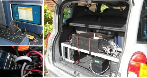
The device owned by the Istituto Motori is a Semtech-Sensor, mounted in the rear of the IV, as shown in the figure below (Figure 6). PEMS can record instantaneous pollutant concentration and exhaust flow data streams at 1 Hz.

Figure 6 –Instrumented Vehicle equipped with PEMS

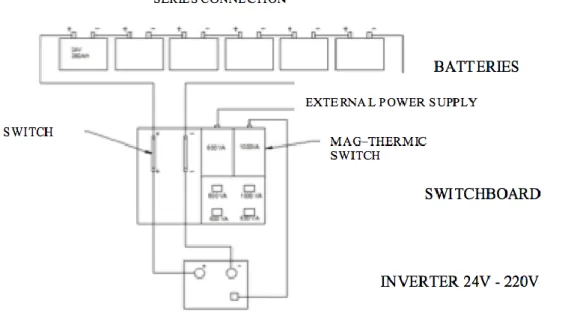
The Semtech is powered by six batteries, each one at 4 V for a total of 24 V. In the Figure 7 is reported the diagram of power supply system, as shown there is a connection in series among the six battery, in order to obtain a voltage of 24V. Moreover this group of batteries is connected to a switchboard, which has two safety switches (one on the positive pole, and the other one on the negative pole).

Figure 7 – Diagram of power supply system of SEMTECH

These two switches also connect the batteries with an inverter; in this way the input tension of 24v is transformed in AC (alternating current) 220v. In this way, it’s possible to supply jacks of switchboard with a nominal power of 1000 VA (Volt-Ampere). The Semtech, and all the devices necessary to carry out the road test, are connected to these jacks (Figure 7).

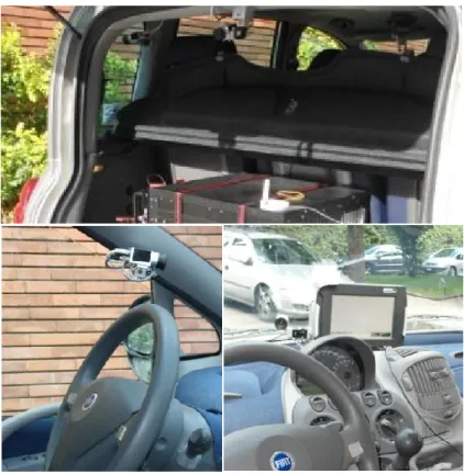
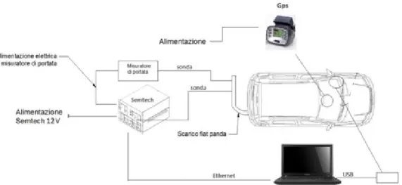
Finally, as illustrated in Figure 8 below, several devices have been mounted on the IV in order to evaluate and record the environment conditions and tailpipe exhaust gas:

- Semtech for the analysis of tailpipe exhaust gas,

- Exhaust Flow Meter measurments (EFM),

- GPS,

Figure 8 – Scheme of devices mounted during the on-road test

2.1.3 Twins Driving Simulators

The two-twins static driving simulators (DSs), owned by the Dipartimento di Ingegneria Civile Edile ed Ambientale (DICEA) were assembled in May 2012 as part of the DRIVE IN2 project. Both the DSs have the same hardware and software in order to enable a complete interaction in the same virtual driving scenario. Each of the cockpits consists on: mono-seat, steering wheel, pedals and gear lever.

The dashboard, the various indicators (as speedometer, fuel level, gear engaged, etc.), and the side/rear-view mirrors are reproduced virtually. The gearshift can be both manual and automatic. All control interfaces provide a realistic response. As an example, the pedals are provided with a dynamic system of force feedback and the torque at the wheel is reproduced with high accuracy by means of a servomotor directly connected to the steering column. The architecture of simulation does not provide a system of motion, because of a fixed base. Three-dimensional images are projected on three 23” screens surrounding the cockpit. Such images immerse the driver in a driving environment realistic that reproduces the road and the surroundings environment (such as houses, vehicles, road signs, trees, etc.) with a high degree of detail. The driving scenarios that can be simulated are varied and include driving at night and in bad weather condition (rain, snow, fog) .The video system ensures a field of front vision of 100°x20° and a total resolution of 5040 x 1050 pixels.

A wrap-around sound system (2 speakers and 1 subwoofer) generates the sounds coming from the driven vehicle (engine, horn, etc.) and from the traffic (other vehicles). A video camera is installed in front of cockpit allowing the researchers to monitor the status of the participants and document the behaviour while driving.

Ultimately, all stimuli provided to the driver can be accurately reproduced so as to ensure the feeling of being in a real vehicle carrying out a real driving task. Furthermore, the quality of video (refresh rate 60 images per second) and audio systems contribute to make the driving experience as realistic and complete as possible.

The DSs use as a driving simulation software SCANER STUDIO Ver. 1.4 developed by OKTAL, which provides a flexible and effective simulation with an advanced traffic model. The software, in fact, allows to simultaneously handle a traffic of more than 200 different types of autonomous vehicles (motorcycles, cars, trucks, buses, emergency vehicles, bicycles and pedestrians). Each vehicle has assigned driving behaviour rules, which interacts with other vehicles during the simulation. These rules can be replaced by others imposed by the requirements of the scenario (example: control logic). To increase the realism of the driving environment, autonomous vehicles of traffic reproduces the dynamic case by means of the roll (during a planimetric curve)

or pitch (during accelerating or braking phases) and, also, they are able to reproduce the visual signals (marker lights, emergency brake lights, turn lights, fog lights, etc.). In order to generate scenarios with high density of traffic it’s possible to create a “swarm” of autonomous vehicles around the interactive vehicle (vehicle controlled by the human driver).

It’s, finally, possible to record a huge variety data, such as: data concerned the inputs of the driver’s control (steering wheel angle, racing pedals, turn signals, gear, etc.), data related to the vehicle (speed, engine speed, position, etc.), information about autonomous vehicles and, at last data useful to define the behaviour in relation to other vehicles and the road infrastructure. According to the needs of the experiment, it’s possible to choose the recording frequency (100Hz max) and the type of data to be recorded.

2.2 Experimental surveys and data collection

In this section the two experimental campaigns have been discussed. In particular the first one involved a large survey (a sample of 100 drivers), while the second one involved 20 drivers. These two experimental campaigns have been fully supported by the DRIVEIN2 project.

2.2.1 DriveIn

experiment

The experiment described in this section has been carried out during the DRIVEIN2 research project that focuses on defining methodologies, technologies and solutions aimed at capturing driving behaviours (Bifulco, Pariota, Galante, & Fiorentino, 2012). The research project was carried out at the Dipartimento di Ingegneria Civile ed Ambientale of the University of Naples and experimental sessions have lasted from September to October 2012. A sample of 100 participants was selected for experimental purposes, drawn in order to match the population of Italian drivers. The following levels were considered in the stratification of the population:

1. Gender: male and female; 2. Age, 4 classes:

 class 1, from 20 to 24 years old;  class 2, from 25 to 40 years old;  class 3, from 41 to 64 years old;  class 4, over 65 years old;

3. Educational level attained, considered low (until high school diploma) or high (after graduation).

The admissible combination of the previous features allows the sample to be split over 14 layers ( Table 1 below).

Layer Age Gender Educational level Relative Incidence Layer Cardinality (over sample of 100) 1 _20-24 M _L 0.2*0.429*1 9 2 F 0.2*0.571*1 11 3 25-40 M L 0.3*0.483*0.5 7 4 H 0.3*0.483*0.5 7 5 _F L 0.3*0.517*0.5 8 6 H 0.3*0.517*0.5 8 7 41-64 M L 0.3*0.491*0.5 7 8 H 0.3*0.491*0.5 7 9 _F L 0.3*0.509*0.5 8 10 H 0.3*0.509*0.5 8 11 ≥65 M L 0.2*0.674*0.5 7 12 H 0.3*0.674*0.5 7 13 _F L 0.3*0.326*0.5 3 14 H 0.3*0.326*0.5 3

Table 1 – The sample

The cardinality of each layer depends on the relative incidence on the population given by official data, such as those provided by the ISTAT (Istituto [Nazionale] di STATistica – Italian National Statistics Institute), as updated to the latest available year. In order to fill in missing information, we also used data from the DATIS project, carried out by the ISS (Istituto Superiore della Sanità – Italian National Health Institute, http://www.iss.it/chis/?lang=2) to define the distribution of gender in each single layer.

Having defined the desired cardinality of each layer, we recruited individuals among those responding to an advertisement requesting volunteers

for a study on driving behaviour. Volunteers have been rewarded with 70 euro for participation to both the on-the-road and the driving simulator sessions. Selection was carried out in three steps:

a) Contact, 100 drivers were needed; however, we decided on a preliminary basis to select 150 drivers, distributed according to the desired stratification. Thus a preliminary sample was considered by increasing each of the sample layers by 50%;

b) Administration of the pre-selection questionnaire to those showing interest in participating in the experiment. This questionnaire consisted of four distinct parts: Personal Data; Traffic Locus Of Control Questionnaire (T-LOC); Marlowe Crowne Social Desirability (MCSD); Dangerous Driving (DDDI).

T-LOC, MCSD and DDDI, were administered in random order to respondents, to avoid distortion phenomena, as most people tend to provide the last answers hastily due to the annoyance. Analysis of the questionnaire responses achieved three purposes:

 it confirmed that the respondents belonged to the layer he/she had

been contacted for. If the layer was not confirmed, the respondent was switched to the appropriate layer. If, after verification of all respondents a layer was under-represented with respect to the desired classification, the sample was supplemented with new respondents;

 it classified the respondents by employment status: student (if

appropriate for the considered layer, depending on age), employed vs. unemployed, retired (if appropriate for the layer);

 it divided individuals into clusters. Three categories were created

according to responses given to the T-LOC, MCSD and DDDI tests by using two-step cluster analysis (TSC, SPSS Inc. 2001): aggressive drivers; aggressive drivers and fatalists; non-aggressive and non-fatalistic drivers;

c) Final selection of the sample: from 150 contacts 100 respondents were selected. For each layer, respondents were selected, obtaining a good balance with respect to employment status and clusters in order to

ensure a representation not lower than 25% for each of three clusters. The experiment was organised into daily experimental sessions, each consisting of several driving sessions. In order to schedule the driving tests, the drivers made their own reservations for one of the experiment day through a web application. Driving sessions were sequenced every two hours, accommodating driving time and the time required to answer two questionnaires (pre and post-driving). Each daily session involved at most five driving sessions (from 8:30 a.m. to 6:30 p.m.). Since the sun sets before 6 p.m. only in last days of October, similar sunlight conditions were established for each session.

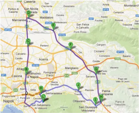
Figure 10 – The experimental path

The following steps were carried out for the observation of each of the 100 drivers:

 each driver drove on the same tour (see Figure 10) by using the instrumented vehicle described previously, detecting the behaviour of the driver with respect to the vehicle ahead and the behaviour of the driver of the vehicle above with respect to the instrumented vehicle;  the tour is 78 km long, each driving session lasting about one hour; the

route consists in a single loop, evolving over three roads near Naples as in Figure 10 for a total length of 60 km:

- National Highway A1 (from B to D in Figure 10, about 14 km), consisting of a dual carriageway and three lanes for each traffic direction, with a designated speed range of 80-120km/h (speed limit 100 km/h). Here the driver is immersed in a traffic stream that moves at about 100 km/h. Thus natural car-following data are obtained, in the sense that the driver is not asked to perform special tasks;

- National Highway A30 (from D to H in Figure 10, about 30 km), with the same characteristics as National Highway A1, apart from the speed limit (130 km/h). Here the driver interacts with a vehicle taking part to the experiment (corporate vehicle), which carries out several standard manoeuvres. In particular, the driver is asked to perform three approaching manoeuvres with the leader at a constant speed of 80, 100 and 120 km/h;

- The "Vesuvius" State Highway SS 268 (from I to K in Figure 10, about 16 km), consisting of a single carriageway with one lane per traffic direction, at-grade intersections and design speed interval of 60-100 km/h (speed limit 90 km/h). Here the corporate vehicle is not present; however car-following data are obtained.

For part of each of the three main sections a workload experiment was carried out on the drivers, aimed at estimating their mental workload. This refers to the portion of the driver’s information processing capacity (or resources) that is actually required to meet requirements in the driving task (Eggemeier, Wilson, Kramer, & Damos, 1991). In particular, Rotated Figures Task (RFT, as in Stanton et al. (1997)) is a self-paced secondary task used to measure performance-based workload. It has been successfully adopted in previous research about workload assessment as a secondary task during driving and its reliability can compensate for its apparent lack of ecological validity. To ensure the effective measure of the spare attentional capacity, this subsidiary task is designed to load the same attentional resources as driving (which are, visual input, spatial processing and manual response; Wickens (2002)). The starting point for driving sessions was Via Gianturco, a major

urban road in the eastern part of Naples, due to the availability of public transport services, thanks to the Gianturco underground station, and quick access to the A1 Highway. Having been met at the beginning of the test-driving route, selected drivers were given a pre-driving questionnaire, comprising the DCQ (Driver Coping Questionnaire) and the DSI-Pre (Driver Stress Inventory-Pre) as described in Matthews et al. (1996) as well as the Italian version of the PANAS (Terracciano, 2003). The tests aimed to investigate the driver’s mood prior to driving and to interpreter his/her driving behaviour in light of it.

Before point B, a period of acclimatization (from L to B in Figure 10) was introduced, where the driver familiarized him/herself with the instrumented vehicle, to prevent the driving behaviour being biased by lack of familiarity. A final section was introduced (from K to L, see Figure 10) allowing the driver to come back to the starting point. Finally, a post-driving questionnaire was posed to drivers in order to ascertain in what way the driver’s mood was influenced by the experiment. The questionnaire comprised the DSI-Post and the NASA-TLX tests adapted for workload ( (Hart & Staveland, 1988), (Bracco & Chiorri, 2006)). Workload was used, amongst others, to validate an associated experiment carried out using a driving simulator, as presented in Bifulco et al. (2013).

2.2.2 DriveIn

experiment add-on

The experiment described in this section is carried out in collaboration with the CNR (Consiglio Nazionale delle Ricerche – Istituto motori)

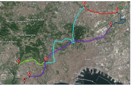
Figure 11 – The experimental path

The route is divided into four main sections, and it is long about 40 km:  The first section, about 4km long, is made up of the urban freeway

“Vomero-Soccavo-Pianura” (Figure 11, green);

 The second section, about 10 km long, is made up of various urban roads that cross several areas of Naples: Vomero, the so called Hospital District of Naples, Colli Aminei, Capodimonte and finally Miano (Figure 11, cyan);

 The third section, 6.5 km long, is the provincial highway 500 “Melito-Scampia” (Figure 11, red);

 The fourth section, about 10 km long, is part of the Autostrada A56, widely known as “Tangenziale di Napoli”, and it is the section in which the higher speeds are reached during the test (Figure 11, purple). The experiment involved a survey of 20 people, randomly sampled. The sample is composed by 4 females and 16 males, with an average age equal to 29.4 years.

Chapter III

–

Fuel consumption

model

Introduction

In this chapter the fuel consumption model is presented and discussed. The model is specified and calibrated thanks to the dataset obtained from the experimental survey of DRIVEIN2 project (paragraph. 2.2.1). The available sample, composed by 100 drivers is randomly split into two groups: the first group is used for specification and calibration purposes, while the second group is employed for testing and validation of the model. Due to the “panel data” typology of the dataset, a linear mixed-effect model is used in order to specify the fuel consumption model. Finally due to the fact that the data are collected using the OBD-II port, as the direct access to the CAN (Controller Area Network) is not allowed, a validation of fuel consumption data collected by the OBD-II port is carried out using a PEMS.

3.1 Linear mixed effect model

For hierarchical data with a single level of grouping, we can formulate the classical LMM (Linear Mixed Model) at a given level of a grouping factor as follows:

𝑦_𝑖 = 𝑋_𝑖𝛽 +⁡𝑍_𝑖𝑏_𝑖 + 𝜀_𝑖 (12

Where

𝒚_𝒊≡ ( 𝒚_𝒊𝟏 ⋮ 𝒚_𝒊𝒋 ⋮ 𝒚_{𝒊𝒏𝒊)} (13

- 𝑋𝑖 is a design matrix for the i-th group:

𝑋_𝑖 ≡ (

𝑥_𝑖1(1) 𝑥_𝑖1(2) ⋯⁡⁡⁡⁡⁡⁡⁡𝑥_𝑖1(𝑛) ⋮ ⋮ ⋱⁡⁡⁡⁡⁡⁡⁡⋮ 𝑥_𝑖𝑛(1)_𝑖 𝑥_𝑖𝑛(2)_𝑖 ⋯⁡⁡⁡⁡⁡⁡⁡𝑥_𝑖𝑛(𝑛)_𝑖

) ≡ (𝑥_𝑖(1)⁡𝑥_𝑖(2)⁡…⁡𝑥_𝑖(𝑝)) ₍₁₄

- 𝛽 are the corresponding regression parameters:

𝛽𝑖 ≡ ( 𝛽_𝑖1 ⋮ 𝛽𝑖𝑗 ⋮ 𝛽_{𝑖𝑛𝑖)} (15

- 𝜀𝑖 the vector of the within-group residuals errors:

𝜀_𝑖 ≡ ( 𝜀_𝑖1 ⋮ 𝜀_𝑖𝑗 ⋮ 𝜀_{𝑖𝑛𝑖)} (16

- 𝑍𝑖 and 𝑏𝑖 are the matrix of covariates and the corresponding vector of random effects:

𝑍_𝑖 ≡ ( 𝑧_𝑖1(1) 𝑧_𝑖1(2) ⋯⁡⁡⁡⁡⁡⁡⁡𝑧_𝑖1(𝑞) ⋮ ⋮ ⋱⁡⁡⁡⁡⁡⁡⁡⋮ 𝑧_𝑖𝑛(1)_𝑖 𝑧_𝑖𝑛(2)_𝑖 ⋯⁡⁡⁡⁡⁡⁡⁡𝑧_𝑖𝑛(𝑞)_𝑖 ) ≡ (𝑧_𝑖(1)⁡𝑧_𝑖(2)⁡…⁡𝑧_𝑖(𝑞)) ₍₁₇ 𝑏𝑖 ≡ ( 𝑏𝑖1 ⋮ 𝑏𝑖𝑞 ) ₍₁₈

Similar to the design matric Xi, the matrix Zi contains known values of q covariates, with corresponding unobservable effects bi. Moreover:

𝑏_𝑖~𝑁_𝑞(0, 𝐷), 𝜀𝑖~𝑁𝑁_𝑖(0, 𝑅𝑖), with 𝑏𝑖 ⊥𝜀𝑖 (19

i.e., the residual errors 𝜀𝑖 for the same group are independent of the random effects bi. This particular assumption plays the key role in distinguishing a classical LMM from an extended one. In addition, we assume the vectors of random effects and residuals errors for different groups are independent of each other, i.e., bi is independent of 𝜀_𝑖′ for i≠i’.

We also specify that

D=σ2𝐷 Ri=σ2 𝑅𝑖 (20

In general, it’s assumed that D and Ri are positive-definite, unless stated otherwise.

As we can see, in addition to the fixed-effects parameters 𝛽 for the covariates used in constructing the design matrix 𝑋_𝑖, model (12) includes two random components: the within-group residual errors 𝜀𝑖 and the random effects bi for the covariates included in the matrix 𝑍_𝑖. The presence of fixed and random effects of known variables justifies the name of model.

In many cases, the random effects included in bi have corresponding fixed effects, contained in 𝛽. Consequently, the matrix 𝑍_𝑖 is often created by selecting

a subset of appropriate columns of the matrix 𝑋_𝑖. In this case, it is said that the corresponding fixed and random effects are coupled. The notation and theoretical part of this section is presented in the book of Gałecki & Burzykowski (2013).

3.1.1 Specification for all data

In this section, the specification of the single-level LMM, given by (12) - (20), is briefly described for all data.

Let 𝑦 ≡ (𝑦₁′_{⁡, 𝑦}

2′⁡, … , 𝑦𝑁′) be the vector containing all 𝑛 = ∑𝑁𝑖=1𝑛𝑖 observed values of the dependent variable (observed values of fuel-consumption, in our case). Similary, let 𝑏 ≡ (𝑏₁′_{⁡, 𝑏}

2′⁡, … , 𝑏𝑁′) and 𝜀 ≡ (𝜀₁′_{⁡, 𝜀}

2′⁡, … , 𝜀𝑁′) be the vectors containing all Nq random effects and n residual errors, respectively.

Define matrices 𝑿 ≡ [ 𝑋₁ 𝑋2 ⋮ 𝑋_𝑁−1 𝑋_𝑁 ] and𝒁 ≡ [ 𝑍1 0 … 0 0 ⋮ 𝑍⋮2 … 0⋱ ⋮ 0 0 ⋯⁡𝑍_𝑁 ] ₍₂₁

as we can observe, Z is a diagonal matrix. Moreover, 𝑋 is of dimension 𝑛⁡𝑥⁡𝑝, while 𝑍 is of dimension 𝑛⁡𝑥⁡𝑁𝑞. Models (12) - (19), can be written for all data as follows:

𝑦 = 𝑿𝛽 + ⁡𝒁𝑏 + 𝜀 (22

With

Where 𝑫 ≡ 𝐼𝑁 𝐷 = [ 𝐷 0 … 0 0 ⋮ 𝐷 ⋮ … 0⋱ ⋮ 0 0 ⋯ ⁡⁡𝐷 ] 𝑹 ≡ [ 𝑅 0 … 0 0 ⋮ 𝑅⋮ … 0⋱ ⋮ 0 0 ⋯ ⁡⁡𝑅 ] (24

Where  denoting the right Kronecker product.

It is worth noting that the particular block diagonal form of matrices Z, D and R, given in (21), (23) and (24), respectively, results from the fact that the single-level LMM, defined by (12) - (20), assumes a particular hierarchy of data of random effects, as explicitly shown in (19). In particular the model assumes that random effects for different groups, defined by level of particular factor, are independent. Informally, we can describe the hierarchy as generated by grouping factors, with one being nested within the other. It’s possible, however, to formulate random-effects models by using the representation (22), with non block-diagonal matrices Z, D and R. This is the case, for instance, of models with crossed random effects; but this part will not be described because is out of the scope.

3.1.2 Maximum-Likelihood Estimation

In this section methods to obtain a set o estimates of parameters 𝛽, 𝜎2_{, 𝜃} 𝐷 and 𝜃𝑅⁡ for the classic LMM are presented. For the classical LMM, the marginal mean and variance-covariance matrix of yi are given as follow:

𝐸(𝑦_𝑖) = 𝑋𝑖𝛽 (25

𝑉𝑎𝑟(𝑦_𝑖) =⁡Vi (𝜎2, 𝜃, 𝑣𝑖) = ⁡ 𝜎2𝑉𝑖(𝜃, 𝑣𝑖) = 𝜎2[𝑍𝑖𝐷(𝜃𝑅)𝑍𝑖′+ 𝑅𝑖(𝜃𝑅⁡, 𝑣𝑖)] (26 Where 𝜃′_{≡ (𝜃}

𝐷′, 𝜃𝑅′). To simplify the notation, we will, in general, suppress the use of 𝜃 and 𝑣𝑖 in the formulae.

𝑦_𝑖~⁡𝑁_𝑛𝑖(𝑋𝑖𝛽, 𝜎2𝑍𝑖𝐷𝑍𝑖′+ 𝜎2⁡𝑅𝑖) (27

The marginal mean value of the dependent variable vector 𝑦_𝑖, is defined by a linear combination of the vectors of covariates included, as columns, in the group-specific design matrix 𝑋_𝑖, with parameters 𝛽. Moreover, the variance-covariance matrix of 𝑦𝑖, consist of two components. The first one, 𝜎2𝑍𝑖𝐷𝑍𝑖′, is contributed by the random effects 𝑏𝑖. The second one, 𝜎2⁡𝑅𝑖, is related to the residual errors 𝜀_𝑖. Hence, strictly speaking, the model employing random effects, specified in (12) - (19), implies a marginal normal distribution, defined in (27) with the variance-covariance matrix of 𝑦_𝑖 given by (26).

The ML estimation involves constructing the likelihood function based on appropriate probability distribution function for the observed data. The unconditional distribution of bi and the conditional distribution of yi given bi, are not suitable for constructing the likelihood function, because the random effects bi are not observed. Instead, estimation of LMM is based on the marginal distribution of yi. In particular the ML estimation is based on the marginal log-likelihood resulting from (27); the log-likelihood can be expressed as follows: ℓ𝐹𝑢𝑙𝑙(𝛽, 𝜎2, 𝜃) ≡ ⁡ − 𝑁 2log(𝜎2) −1 2⁡∑ log[𝑑𝑒𝑡(𝑉𝑖)] − 𝑁 𝑖=1 1 2𝜎2⁡∑(𝑦𝑖− 𝑋𝑖𝛽)′𝑉𝑖−1 𝑁 𝑖=1 (𝑦𝑖− 𝑋𝑖𝛽) (28

Where Vi, defined in (26), depends on θ and it represents the model-based marginal variance-covariance .

The log-profile-likelihood results from plugging into (28) the estimators of 𝛽 and 𝜎2_{, given by:}

𝛽̂(𝜃) ≡ (∑ 𝑋_𝑖′_𝑉 𝑖−1 𝑁 𝑖=1 𝑋_𝑖) −1 ∑ 𝑋_𝑖′_𝑉 𝑖−1 𝑁 𝑖=1 𝑦_𝑖 (29 𝜎̂_𝑀𝐿2 _{(𝜃) ≡ ∑ 𝑟} 𝑖′𝑉𝑖−1𝑟𝑖⁄𝑛 𝑁 𝑖=1 (30 Where 𝑟_𝑖 ≡ 𝑟_𝑖(𝜃) = 𝑦_𝑖 − 𝑋_𝑖𝛽̂(𝜃).

By maximizing the log profile- likelihood function over 𝜃, we obtain estimators of these parameters. Plugging 𝜃̂ into (29) and (30) yields to corresponding estimators of 𝛽⁡and 𝜎2_{, respectively.}

The ML estimates of the variance-covariance are biased. For this reason, the parameters are better estimated using the REML (Restricted Maximum Likelihood) estimation. Toward this end, the log-restricted-likelihood function is considered, in particular: ℓ∗ 𝑅𝐸𝑀𝐿(𝜎2, 𝜃) ≡ ⁡ ℓ𝐹𝑢𝑙𝑙(𝛽̂(𝜃), 𝜎2, 𝜃) +⁡ 𝑝 2log(𝜎2) −1 2⁡log [𝑑𝑒𝑡 (∑ 𝑋𝑖′𝑉𝑖−1 𝑁 𝑖=1 𝑋_𝑖)] (31

Where 𝛽̂(𝜃) is specified in (29). From this function, the parameter 𝜎2 _is profiled out by replacing it by the following estimator, corresponding to:

𝜎̂_{𝑅𝐸𝑀𝐿}2 _{(𝜃) ≡ ∑ 𝑟}

𝑖′𝑉𝑖−1𝑟𝑖⁄(𝑛 − 𝑝) 𝑁

𝑖=1

(32

This leads to a log-profile-restricted-likelihood function, which only depends on 𝜃:

ℓ∗ 𝑅𝐸𝑀𝐿(𝜃) ≡ ⁡ − 𝑛 − 𝑝 2 log (∑ 𝑟𝑖′ 𝑁 𝑖=1 𝑟𝑖) − 1 2⁡∑ log[𝑑𝑒𝑡(𝑉𝑖)] 𝑁 𝑖=1 −1 2⁡log [𝑑𝑒𝑡 (∑ 𝑋𝑖′𝑉𝑖−1 𝑁 𝑖=1 𝑋_𝑖)] (33

Maximization of (33) yields an estimator of 𝜃, which is then plugged into (29) and (32) to provide estimators of 𝛽⁡and 𝜎2_{, respectively.}

3.2 Validation of OBD fuel consumption

Validation of consumption data is a fundamental pre-requisite of research, as it represents the reference quantity of that research. The OBD port is the unique communication port that has been adopted for obtaining data from the vehicle. From one hand this is a deliberate choice, as we are interested in adopting a variable that can be collected with ease; from the other hand, data obtained from the OBD-II port have lower quality than data that can be directly accessed via the CAN (Controller Area Network) of the vehicle. In our case the direct access to the CAN was not allowed. In case the car-maker allows for the access to CAN (or the solution is directly applied by the car-maker), the quality if the observed data should be a less significant issue.

In our context, the validation of the reliability of collected FCinst has been carried out indirectly. It is straightforward to obtain FCinst from Fuel metering [mg i] by using the following formulation:

𝐹𝐶𝑖𝑛𝑠𝑡[ 𝑙 𝑠] = 4 ∗ 𝑅𝑃𝑀 ∗ 𝐹𝑢𝑒𝑙⁡𝑀𝑒𝑡𝑒𝑟𝑖𝑛𝑔 2 ∗ 1000 ∗ 60 ∗ 825 (34 where:

 4 is the number of cylinders in the engine;

 RPM is rated for two because we have one injection each 2 RPM;

 Fuel Metering, which represents the milligrams of fuel consumed inside the combustion chamber for each injection cycle measured in that instant;

 1000 is used to switch from mg to g;

 60 is the number of seconds in one minute; and  825 is the density of diesel fuel (g/l).

Indeed a direct correlation exists between fuel consumption and emissions. Thus, measuring emissions allows for an indirect estimation of fuel consumption, thanks to stoichiometric relationship among fuel burnt, carbon monoxide and carbon dioxide emitted. For this purpose the following formulation are used:

𝐹𝐶𝑃𝐸𝑀𝑆[ 𝑙 𝑠] = 0.116 0.8242⁡ 0.273⁡𝑥⁡𝐶𝑂2+ 0.429⁡𝑥⁡𝐶𝑂 100 (35

where CO2 and CO are respectively the instantaneous mass of carbon dioxide and carbon monoxide expressed in g/s. In other words 0.273 is the carbon mass fraction of CO2, CO2 is the carbon dioxide in g/s, 0.429 is the carbon mass fraction of CO and CO is the carbon monoxide expressed in g/s. Finally for vehicle fuelled with diesel 0.116 is a balance parameter and 0.8242 is the density of tested fuel at 15°C in kg/l. The development of this formulation is an outcome of experiments carried out for the DRIVE IN2project by the Istituto Motori of the National Research Council (CNR) of Italy.

The first step to perform, in order to compare the consumption data come from different instruments, consists on the data tuning. The lowest common denominator of data collected during the transferability experiment is the GPS signal. As the GPS, not only report the exact time, gets the speed profile also; which can be compared with the speed profile collected by the OBD port and with the flow rate of the exhaust gases that has the same form of speed profile for less than a scale factor. Applying this procedure for each driver, involved in this experiment, the data collected by the OBD are in tune with the data collected by the PEMS.

It is here reported absolute percentage error between the fuel consumption collected by the OBD port and the consumption obtained starting from the