Published online in Wiley InterScience (www.interscience.wiley.com). DOI: 10.1002/asmb.592
The value of simple models in new product forecasting
and customer-base analysis
Peter S. Fader
1,*
,y,}and Bruce G. S. Hardie
2,z,}1The Wharton School of the University of Pennsylvania, 749, Huntsman Hall, 3730 Walnut Street, Philadelphia, U.S.A.
2London Business School, U.K.
SUMMARY
In this paper, we develop the idea of a ‘simple model’}defined as one that a good business student can build and implement on his/her notebook PC using readily available software. We explore how such models have the potential to bridge the gap between what marketing academics create and what marketing managers seek in a model. We provide specific examples from the areas of new product sales forecasting and customer-base analysis, using spreadsheet-based models that provide good forecasts and insights about actual buyer behaviour. Copyright#2005 John Wiley & Sons, Ltd.
KEY WORDS: new product sales forecasting; customer-base analysis; repeat buying; spreadsheet modelling; model implementation
1. INTRODUCTION
When reflecting on the increasing gap between what marketing academics create and what marketing managers seek in a model, we often focus on the ‘supply side’, discussing how the academic incentive structure rewards the development of increasingly new (and more complex) methodologies with little or no thought given to ease of implementation. However, let us consider the ‘demand side’: why are managers not rushing to use the models that we, as academics, develop?
* They do not understand how our (increasingly complex) models work; few managers have
the mathematical and/or statistical training to understand what lies behind our models. If a
*Correspondence to: Peter S. Fader, Department of Marketing, The Wharton School of the University of Pennsylvania, 749 Huntsman Hall, 3730 Walnut Street, Philadelphia, PA 19104-6340, U.S.A.
y
E-mail: [email protected]; (url: www.petefader.com) z
E-mail: [email protected]; (url: www.brucehardie.com) }Frances and Pei-Yuan Chia Professor of Marketing. }Associate Professor of Marketing.
Contract/grant sponsor: London Business School
manager has had no exposure to the benefits that can be derived from a good marketing model, it is natural for him to be suspicious of ‘black-box’ solutions.
* Even if a manager truly understands and appreciates the value of models, he still has to
convince other people within his organization. Faced with a sceptical set of colleagues, the manager needs to be able to convey the logic of the models in their own language. And even if the manager is successful in conveying the logic, requests for funds to implement an ‘academic’ model are typically met with limited enthusiasm.
* The implementation of our models typically requires (relatively) sophisticated modelling
skills, including custom programming and non-standard data manipulation. Fewer and fewer companies have specialized departments in which such skills can reside. And realistically speaking, it is not the marketing manager’s job (or that of his/her immediate subordinates) to acquire such skills.
Rather than wring our hands in despair, we say ‘If you can’t take Mohammed to the mountain, take the mountain to Mohammed’. Rather than rely on the traditional diffusion process for new market research ideas [1] in which academics develop their models and rely on market research providers and specialist consultants to bridge the gap, we suggest that models be developed from scratch with a clear focus on the types of issues/constraints mentioned above. This results in what we call ‘simple models’. In the next section, we define what we mean in practice by the term ‘simple model’. To provide specific examples, we discuss our work on developing models for new product sales forecasting and customer-base analysis.
2. THE NOTION OF A ‘SIMPLE MODEL’
A ‘simple model’ is one that a good business student}even with a non-technical
background}can build and implement on his/her notebook PC using readily available
software.
This focus on a good business student, even with a non-technical background, is an important aspect of our notion of a simple model. In our own experience, we are typically dealing with MBA students whose professors in the more quantitative core courses (such as finance and management science) have not ‘dumbed-down’ the material, but rather made sure that everyone is up to a common standard. With such foundations in place, the presence or absence of a technical background becomes less relevant.
‘Readily available software’ includes a spreadsheet package with standard optimization add-ins, possibly augmented by popular third-party add-ins for Monte Carlo simulations. If a formal statistics package is to be included under the heading of readily available software, we would consider the basic packages widely used in undergraduate teaching. Experience suggests that such packages are far more likely to be present in a typical corporate environment than the more advanced ones used by post-graduate students and researchers.
It is important to note that we arenottalking about the ability to deliver/deploy the model to
the end-user in a spreadsheet. Rather, we are talking about the need for the manager to be able tobuild the model for himselfstarting with a blank spreadsheet. Building the model from scratch in a spreadsheet helps the user learn about the model structure. It is one thing to read a paper or
attend a conference presentation about a model; it is quite another thing to actually build the model from scratch. The confidence that comes from this exercise empowers the manager, eliminates the black-box aspect of many models, and makes it much more likely for the model to be able to successfully diffuse through an organization.
It must also be noted that our notion of a simple model focuses on ability of the end-user to implement the model (with an implicit recognition that it should not be too difficult for this person to understand the logic of the model). ‘Simple’ should not be viewed as a synonym of naı¨ve, as is often the case in discussions of what constitutes a good model. (We visit this issue in Section 5.)
In our own models of new product sales and customer-base dynamics, the underlying data sets share a common structure, featuring information about the series of transactions at the level of the individual customer. See Figure 1. The management of such data sets, especially for modelling purposes, is not an easy task for the novice, and doing so using a standard spreadsheet or statistical package is not very straightforward or convenient. The manipulation of the data required for model implementation (e.g. parameter estimation) is a major barrier faced by our prototypical model builder/implementer. This leads to another defining characteristic of a simple model in many settings:
In many situations, a ‘simple model’ makes use of data summaries.
Examples of such summaries are given in Tables I–III, which contrast sharply with the detailed transaction-by-transaction data structure portrayed in Figure 1. In Section 3, we explore the development of spreadsheet-based models for forecasting new product sales based on a summary of the form given in Table I. In Section 4, we discuss two spreadsheet-based models for customer-base analysis that use data summaries of the form given in Tables II and III. (Copies of the spreadsheets associated with these three models, along with supporting documentation, are available from the authors.)
3. FORECASTING NEW PRODUCT SALES
At the heart of any new product sales forecasting model is a multiple-event timing process that accounts for cross-sectional heterogeneity as well as non-stationarity in underlying buying rates
Person 1
Person 2
Person 3
Person n
time 0 time1
(due to the temporary effects of marketing mix variables and the evolution of consumers’ preferences for the new product as they gain more experience with the product). The correct way to model such a multiple-event process is to first condition on the individual and then account for cross-sectional heterogeneity [2]. However, such ‘correct’ models (e.g. Reference [3]) require data on the timing of the trial, first repeat, second repeat, and so on transactions for each customer (i.e. as illustrated in Figure 1) and require the use of specialist mathematical modelling environments for model implementation. (The ‘trial’ purchase is the customer’s first-ever purchase of the new product. The ‘first repeat’ purchase is her first post-trial (i.e. second-ever purchase) of the new product. And so on.)
Central to tracking and understanding the performance of a new product is the decomposition of aggregate sales into its trial and repeat components,
SðtÞ ¼TðtÞ þRðtÞ
where, assuming for presentational simplicity that only one unit is purchased on each purchase
occasion,SðtÞis the cumulative sales volume up to timet;TðtÞis the cumulative number of triers
up to timet;andRðtÞis the total number of repeat purchases up to timet:
According to the so-called depth-of-repeat decomposition [4],
RðtÞ ¼X
1
j¼1 RjðtÞ
where RjðtÞ is the number of consumers who have made at least j repeat purchases of
the new product by time t: Standard performance metrics such as ‘percent triers repeating’
and ‘repeats per repeater’ [5, 6] are easily computed from these data. At any point in time t;
percent triers repeating is computed as R1ðtÞ=TðtÞ; while repeats per repeater is computed
as RðtÞ=R1ðtÞ:
Therefore, one way of summarizing the customer-level transaction data for a new product is to determine the number of triers, first repeaters, second repeaters, and so on over time. In Table I, we report these data for ‘Kiwi Bubbles’, a masked name for a shelf-stable juice drink. Prior to its national launch, the Kiwi Bubbles product underwent a year-long test using
Information Resources, Inc.’s BehaviorScan1 testing service. (This table summarizes the
purchasing of the new product by 1499 households in one market over the first 24 weeks of the
test.) Each column reports the cumulative number of panellists that have made a trialðDoR¼0Þ
purchase, a first repeatðDoR¼1Þpurchase, and so on for each of the 24 weeks.
Such a summary is easy to create from the raw transaction data}in fact this was done in a
spreadsheet making use of the ‘pivot table’ facility. Assuming a sufficiently fine time period, such a table can be created using the panel tracking reports provided by companies such as ACNielsen, Taylor Nelson Sofres, and Catalina Marketing. The important thing to note is that this type of summary is fairly easy to manage in a spreadsheet environment. The question is
whether it lends itself to be the key input for a successful forecasting model}can we create an
accurate sales forecast given just the data presented in Table I?
The answer, from our experience, is a clear yes. Building on the seminal work on test market forecasting models [4, 7, 8], it is possible to develop a simple sales forecasting model entirely in a spreadsheet that simply uses the data presented in Table I.
The key idea is to build separate sub-models for trial, first repeat, second repeat, and so on, each of which is ‘built’ in a separate worksheet within a single spreadsheet workbook. That is,
the first model captures (and forecasts) time to trial, the second model captures (and forecasts) time to first repeat, and so on. As we transition from trial to first repeat, the only piece of information we effectively retain about each person is that they made a trial purchase; we do not
take into account when they made that prior purchase. This is clearly an ‘incorrect’ way of
modelling the multiple-event timing data summarized in Table I since it does not utilize the complete behavioural history up to that point.
As determined in a recent model ‘bakeoff’ [9], the best trial model, in terms of forecasting accuracy, is the simple exponential-gamma (EG) timing model. However, to maximize understanding of the basic model, ‘Version 1.0’ of the model based on the Table I data uses the exponential with ‘never triers’ (ENT) model, a continuous-time analogue of the basic Fourt and Woodlock model, which is almost as good as the EG model [9]. Furthermore, instead of estimating the trial model parameters using the method of maximum likelihood (MLE), we apply non-linear least-squares (NLS) to the cumulative trial curve. Given our prototypical modellers’ high comfort-level with the logic of least-squares estimation in other contexts, this
change lets them stay more focused on the model, per se, rather than on the parameter
estimation method. In our efforts to get a manager on board with model development, we much prefer to use an estimation method that might not have all the theoretical/asymptotic niceties
Table I. The cumulative number of panelists (out of a panel of 1499 households) who have made a trial ðDoR¼0Þpurchase, a first repeatðDoR¼1Þpurchase,. . .;a seventh repeatðDoR¼7Þpurchase of ‘Kiwi
Bubbles’, a shelf-stable juice drink, for each of the first 24 weeks of the test market. Depth of repeat level
Week 0 1 2 3 4 5 6 7 1 8 0 0 0 0 0 0 0 2 14 1 0 0 0 0 0 0 3 16 2 0 0 0 0 0 0 4 32 3 0 0 0 0 0 0 5 40 7 0 0 0 0 0 0 6 47 9 2 0 0 0 0 0 7 50 12 2 1 0 0 0 0 8 52 13 2 1 1 0 0 0 9 57 17 4 2 1 0 0 0 10 60 18 6 2 1 0 0 0 11 65 22 8 4 1 0 0 0 12 67 23 9 4 1 1 0 0 13 68 23 9 5 1 1 0 0 14 72 23 10 5 2 1 0 0 15 75 23 11 5 2 1 0 0 16 81 24 13 5 2 1 0 0 17 90 24 15 7 2 1 1 0 18 94 28 15 9 4 1 1 0 19 96 32 16 9 5 1 1 0 20 96 33 18 9 5 2 1 0 21 96 33 18 11 5 2 2 0 22 97 34 18 11 5 2 2 1 23 97 35 18 11 5 2 2 2 24 101 35 20 12 5 2 2 2
that MLE may enjoy, but instead enhances the user’s understanding of the behavioural ‘story’ we are trying to tell.
The basic repeat model uses methods first discussed by Eskin [4] and Kalwani and Silk [8]. Their ideas of how the parameters for the sub-models that govern the transition from first repeat to second repeat, from second repeat to third repeat, and so on, are easily implemented in a simple spreadsheet. In terms of parameter estimation, the procedure proposed by Eskin is rather cumbersome, and Kalwani and Silk’s MLE procedure suffers from the need to have a separate triangular matrix of transition times for each depth-of-repeat level, as opposed to a single column of data as shown in Table I. To the seasoned modeller, this may seem trivial. However, the difference is major for our prototypical business student. With NLS, once we get through the estimation of the trial model, it is easy to extend the same simple logic to the repeat sub-models.
This basic model does a reasonable job of forecasting, and we have found that MBA-level audiences can easily grasp both the intuition and mechanics of the model. Starting with just Table I and a blank spreadsheet, the whole model can be developed from scratch in a single 90-minute class session.
With more time available, we can begin to move towards ‘Version 1.1’, which offers some natural extensions such as moving from the basic ENT model to the EG model.
Absent from our discussion so far is the notion of marketing mix variables. For introductory purposes, we choose to ignore them as they only serve as an additional barrier to understanding the basic model. Furthermore, provided there are enough data points, our research suggests that the inclusion of marketing covariates to the basic model has a negligible impact on aggregate forecasting performance. (Of course, such an omission means that when we use the panel-based forecast to come up with a national sales forecast, we have to assume that the test-market
conditions}including own and competitive marketing activity}will be replicated during the
national launch.)
Once the modeller is comfortable with Versions 1.0 and 1.1, some of these features can be added to the basic models. For instance, we can provide a table that contains a week-by-week summary of the marketing activity (and perhaps competitive actions), which can then be incorporated into the same framework [10].
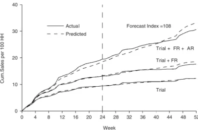
Figure 2 illustrates the forecasting performance of this ‘Version 2.0’ with-covariates model, comparing the total sales forecast (along with its trial and first repeat components) with the corresponding actual sales numbers for the Kiwi Bubbles example. At the year end, we see that the model projections are within 10% of the actual for total sales (and each of its components). As noted above, we can view these models as being ‘incorrect’ as the use of separate sub-models for trial, first repeat, and so on, fails to model the multiple-event process by first conditioning on the individual [2]. As might be expected, this may often yield biased insights into the underlying consumer behaviour, even though the models consistently yield accurate forecasts of aggregate purchasing behaviour [11]. Those users solely interested in forecasting are often willing to stop with this ‘incorrect’ but easy to implement model, rather than migrate to a more ‘correct’ yet more difficult to implement model, such as that presented in Reference [3]. Such users feel that any minor improvements in forecasting accuracy associated with the more correct model do not outweigh the incremental costs of implementation. However, if the goal is to gain insights into the underlying consumer behaviour, it is wrong to use the simple models outlined above. It is important that both model developers and model users be aware of such limitations.
4. CUSTOMER-BASE ANALYSIS
Faced with a database containing information on the frequency and timing of transactions for a list of past customers, it is natural to ask questions such as:
* How many of the customers can be viewed as being active?
* Which customers are most likely to be inactive?
* How many transactions can be expected next period (e.g. year) by those customers listed in
the database, both individually and collectively?
Models are central to answering these customer-base analysis questions, particularly since some of these issues, e.g. the times that customers become inactive, are unobservable. As with the new product forecasting models, a multiple-event timing process lies at the heart of such models, with the need to account for cross-sectional heterogeneity and non-stationarity in the underlying buying rates. (An extreme form of change in buying rate is the customer becoming inactive.) As such, the ‘correct’ models tend to require the full transaction history for each customer and therefore suffer from the data manipulation and model implementation problems discussed above.
We will consider two models that vary in their degree of simplicity (and therefore in their ability to address the above questions). In both cases, the empirical analysis was undertaken using data for a single cohort of new customers who made their first purchases at the CDNOW web site in the first quarter of 1997. We have data covering their initial (trial) and subsequent (repeat) purchase occasions for the period January 1997 through June 1998, during which the 23 570 Q1/97 triers bought just over 115 000 CDs after their initial purchase occasion.
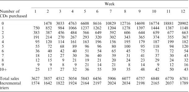
In our first model [12], we chose to work with the summary of total purchasing given in Table II. This includes the distribution of the number of units purchased for each of the
0 4 8 12 16 20 24 28 32 36 40 44 48 52 Week 0 10 20 30 40 Cum.Sales per 100 HH Actual Predicted Trial Trial + FR Trial FR + AR Forecast Index =108
Figure 2. Comparing the cumulative sales forecast (and its components) from the Version 2.0 model with the corresponding actual sales numbers (Trial¼first-ever purchase of the new product, FR¼first repeat (i.e. second-ever) purchase, AR¼additional repeat (i.e. second repeatþthird repeatþ ) purchases).
12 weeks, details of total purchasing, and the number of new customers (triers) in each week. In estimating our model, we used no information beyond these aggregate numbers.
While this is a very convenient summary of the customers’ purchasing, it suffers from two
critical}but managerially realistic}shortcomings: (1) we had no explicit information on the
breakdown of first versus repeat sales in each week, and (2) we could not see the longitudinal series of purchase events at the customer level, which made it impossible to construct a standard model of repeat purchasing (e.g. depth-of-repeat as used in our previous new product sales forecasting example). We therefore had to develop a model of week-by-week repeat purchasing whose parameters could be estimated using the above data.
The model we developed had the objective of forecasting collective purchasing by the cohort of customers. Weekly sales were modelled using a finite mixture of beta-geometric distributions with a separate time-varying component to capture non-stationarity in buying. The perfor-mance of this model is impressive: using the first twelve weeks of data for model calibration and then projecting repeat purchasing out to a 78-week future horizon, we found that the predicted and actual sales curves tracked each other within a tolerance of 5%. The best aspect of this model is that it only requires the purchasing data to be presented in a summary aggregate form (i.e. Table II) and can be implemented completely within a simple spreadsheet.
Readers familiar with the marketing literature on stochastic models of buyer behaviour may wonder why we used the beta-geometric distribution as the underlying counting distribution, instead of the more common NBD (negative binomial distribution) that is widely used within marketing [13]. In this particular setting, there was no underlying reason as to why we should favour one model over the other (cf. the counting of the number of events in a given time period, in which case we would choose the NBD given its link to exponential inter-event times). In this
Table II. Week-by-week distributions of unit purchasing by Q1/97 new customers at CDNOW.n Week Number of CDs purchased 1 2 3 4 5 6 7 8 9 10 11 12 0 1478 3033 4763 6608 8616 10829 12716 14698 16774 18881 20902 1 750 852 984 1066 1237 1262 1204 1278 1397 1444 1387 1148 2 383 387 456 484 566 649 592 606 644 659 677 663 3 191 214 270 267 293 320 302 343 365 374 355 367 4 95 120 114 161 163 196 156 195 179 187 199 182 5 55 72 68 89 96 96 80 100 95 118 94 120 6 36 40 42 40 51 54 65 45 75 71 72 54 7 18 12 27 30 36 40 39 31 41 37 30 43 8 12 15 9 21 19 21 20 24 23 29 24 32 9 9 9 8 9 21 14 21 8 14 9 12 16 10þ 25 17 27 32 36 55 39 35 48 42 50 43 Total sales 3627 3857 4512 5054 5843 6456 5906 6077 6757 6848 6770 6781 Incremental triers 1574 1642 1822 1924 2164 2197 2024 2034 2198 2165 2037 1789 n
Reprinted by permission, Peter S. Fader and Bruce G.S. Hardie. Forecasting repeat sales at CDNOW: a case study.
InterfacesPart 2 of 2 (May–June) 2001;31:S94–S107. Copyright 2001, the Institute for Operations Research and the Management Sciences, 7240 Parkway Drive, Suite 310, Hanover, MD 21076 U.S.A.
particular setting, the beta-geometric provided a better fit to the data. Furthermore, the logic of the beta-geometric distribution is much easier to communicate to a managerial audience, using a coin-flipping analogy, than the rationale for the NBD model (Poisson purchasing at the individual level with gamma heterogeneity). In teaching this model to an MBA-level audience, the behavioural story becomes a highlight of the discussion rather than the technical morass that often arises when we try to get managers to understand a Poisson process. This is important as the chance of managers accepting a model increases with their ability to understand the workings of the model, at the very least at an intuitive level.
Despite its good aggregate performance, a problem with this model and its associated data structure is that we treat the data as a series of cross-sections; we do not model the longitudinal series of purchase events at the level of the individual customer. Consequently, we are unable to make customer-level predictions of future behaviour or to profile individual customers. Although such activities are vital to many customer-base analysis exercises, the required models are generally quite complex and must be calibrated using customer-level data (i.e. like Figure 1) and specialized software. The challenge facing the model developer is to come up with a simple customer-level data structure and a (relatively) simple model that can take advantage of this summary.
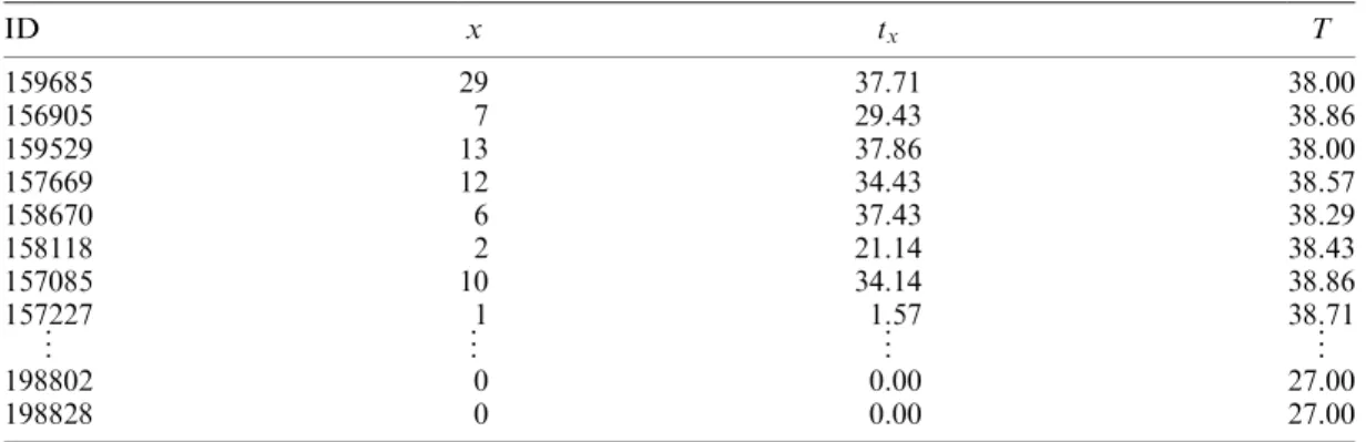
Within the fields of direct and database marketing, it is common to summarize a customer’s behaviour in terms of three summary measures: Recency, Frequency, and Monetary value. In Table III, we report a summary of each CDNOW customer’s transaction history: the length
of the time period during which transactions could have occurred (T), frequency (the number
of transactions in this period, x), and recency (the time of his last transaction,tx). While such
a summary is not quite as concise as those discussed above (Tables I and II), it is still manageable within a spreadsheet environment by someone who is comfortable with the ‘simple models’ covered up to this point. (We are ignoring the monetary value (M) component of the customer’s behaviour. Basic stochastic models for this component [14, 15] can easily be implemented within a spreadsheet environment.)
The challenge facing the model developer is to come up with a model that can be used to answer relevant customer-base analysis questions and for which the R and F summary measures
Table III. Summarizing customer-level repeat buying behaviour at CDNOW in terms of ‘recency’ and ‘frequency’:xis the number of transactions (i.e. frequency) observed in the time periodð0;T;where 0 corresponds to the time of the customer’s first-ever purchase at CDNOW, andtx(05tx4T) is the
time of the last transaction (i.e. recency).
ID x tx T 159685 29 37.71 38.00 156905 7 29.43 38.86 159529 13 37.86 38.00 157669 12 34.43 38.57 158670 6 37.43 38.29 158118 2 21.14 38.43 157085 10 34.14 38.86 157227 1 1.57 38.71 .. . .. . .. . .. . 198802 0 0.00 27.00 198828 0 0.00 27.00
are sufficient statistics. The first model to meet these criteria is the Pareto/NBD ‘Counting
Your Customers’ framework originally proposed by Schmittlein et al. [16], hereafter SMC.
This model was developed to describe repeat-buying behaviour in a setting where customers buy at a steady rate (albeit in a stochastic manner) for a period of time, and then become inactive. More specifically, time to ‘dropout’ is modelled using the Pareto (exponential-gamma mixture) timing model; but while the customer is still active/alive, his repeat-buying behaviour is modelled using the NBD counting model. The Pareto/NBD is a powerful model for customer-base analysis, but its empirical application can be challenging, especially in terms of parameter estimation.
Perhaps because of these operational difficulties, relatively few researchers actively followed up on the SMC paper soon after it was published (as judged by citation counts). But it has received a steadily increasing amount of attention in recent years as many researchers and managers have become concerned about issues such as customer churn, attrition, retention, and customer lifetime value. While a number of researchers refer to the applicability and usefulness of the Pareto/NBD, only a handful claim to have actually implemented it. Nevertheless, some of these papers (e.g. References [14, 17]) have, in turn, become quite popular and widely cited themselves.
In Reference [18], we develop the beta-geometric/NBD (BG/NBD) model, which represents a slight variation in the behavioural story that lies at the heart of SMC’s original work, but it is easier to implement. We show, for instance, how its parameters can be obtained quite easily using a standard spreadsheet package, with no appreciable loss in the model’s ability to fit or predict customer purchasing patterns. Our illustrative empirical application of the model compares and contrasts its performance to that of the Pareto/NBD using the data presented in Table III. The two models yield very similar results, leading us to suggest that the BG/NBD might be viewed as an attractive alternative to the Pareto/NBD in any empirical application, making models for customer-base analysis more broadly accessible so that many researchers and practitioners can benefit from the original ideas of SMC.
It should be noted that R(ecency) and F(requency) are sufficient statistics of a customer’s transaction history for both the Pareto/NBD and BG/NBD models. As such, no sacrifices are made with respect to model ‘correctness’ so as to be able to base the model off an easy-to-handle data summary.
A model such as the BG/NBD cannot be viewed as the final word on customer-base modelling. It ignores the impact of marketing activities on purchasing behaviour. While it is easy to develop such an extension to the basic model, it comes at the cost of ease of implementation, requiring access to specialized mathematical modelling software.
5. REFLECTIONS
At the outset of this paper we referred to the increasing gap between what marketing academics create and what managers seek. It is important to emphasize that this is not a new problem. Writing more than 30 years ago, Urban and Karash [19, p. 62] commented on the gap that already existed at that time and predicted its further growth:
Although there are sophisticated management science models, very few complex ones have achieved continuing use. The problem with implementing these models is significant and will
become more difficult as even more complex management science models and information systems are developed. Difficulties that will occur include: (1) gaining management attention, understanding, and support, (2) limited availability of data to support models, (3) high risk because of large fund commitments, and (4) long model development periods, which will not allow demonstration of short-term benefits.
Their solution was the adoption of an evolutionary approach to the development of marketing models:
The introduction of models as an evolutionary development from simple to more complex but a related one would foster managerial acceptance, encourage an orderly development of data and analysis systems, and reduce risks of failure.
It is our contention that one way to start reducing this gap is not only to get simple models into the hands of the managers, but also to get managers to build the models by themselves.
The thought of building models in a spreadsheet and of using data summaries is not entirely new. Spreadsheet software has played a central role in the use of marketing models in practice [20]. Likewise, the use of data summaries (or ‘data squashing’ [21]) to overcome hardware and software constraints is starting to be explored by data miners.
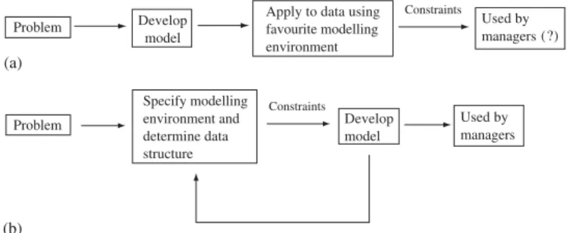
These changes in data handling techniques reflect a different type of model building process. As illustrated in Figure 3(a), the standard model building process starts with the management problem being studied. The model builder develops his model and applies it to data using his standard suite of modelling tools. However, the custom programs, specialist modelling environment and complex data structures serve as barriers to implementation in the firm.
In sharp contrast, the process of building a ‘simple model’ considers the modelling environment and data management constraints at the beginning, and these help guide the development of the formal model, as illustrated in Figure 3(b). Sometimes, the exact nature of the data structures will have to be modified as a result of the mathematical model
developed}maybe simplifications are possible, or maybe more complex data structures are
needed. The emphasis is on developing a model that is both easy to communicate to the manager and easy to implement. The downside is that this can sometimes come at the cost of technical precision.
Problem Develop model
Apply to data using favourite modelling environment Constraints Constraints (?) (a) Problem Specify modelling environment and determine data structure Develop model Used by managers Used by managers (b)
It is important to reflect on our use of the word ‘simple’ when describing a model-building effort. Sometimes the focus is on keeping the number of variables small [22, pp. 102–105]; this reflects much of the philosophy of science and econometrics literature in which simplicity is equated with the number of parameters in the model. A comprehensive discussion of this view of simplicity (and related concepts such as parsimony) is beyond the scope of this paper, and the
interested reader is referred to the recent book Simplicity, Inference and Modelling [23] for a
detailed discussion of the key ideas by philosophers, mathematicians, econometricians, and economists.
Another stream of literature that has explored notions of simplicity is that on the effectiveness of management science interventions. Ward [24] formalized a number of the learnings via the encompassing notions of ‘model transparency’ and ‘constructively simple models’. In this paper, we have focused on the idea of a reasonably qualified end-user being able to build and implement the model on his/her notebook PC using readily available software. (This is very much in the spirit of the call for ‘end-user modelling’ by a number of management science educators [25].) As such, simple does not mean naı¨ve. Nor does it necessarily mean a smaller number of parameters: the ‘simple’ new product sales forecasting models discussed in Section 3 actually have more parameters than a more complex competing model [3].
The value of our so-called ‘simple models’ is manifest in a number of areas:
* As noted earlier, the process of building the model from scratch in a spreadsheet
helps the user learn about the model structure. The confidence that comes with this empowers the manager and removes the black-box aspect of many models. Such an understanding means that it is more likely the model will actually be used by the analyst and decision maker, even if the manager ends up delegating much of the model-building activity.
* The structure associated with the model forces the manager to think in a more logical/
structured/rigourous manner about the problem being addressed. In and of itself, this is of value to the manager.
* Simple models can be implemented at a relatively low cost.
* Finally, they can create subsequent demand for more sophisticated models and the services
of model builders, provided the simple models add substantial value to the organization in the first place. As the user gains experience with a simple model, it is common for him to start asking more from the model than it is designed to deliver. But once he is more familiar with the language and logic of models, we can have intelligent discussions about more complex models. As such, simple models are to be viewed as a starting point, not the final word. Our long-run goal is to move the manager towards more sophisticated methodology, provided the benefits outweigh the costs.
The last point is basically the same message conveyed in the earlier quote from Urban and Karash, so maybe we are just watching history repeat itself. But we sincerely believe that our tangible definition and examples of simple models will provide a starting point to make this evolutionary process a reality. We are encouraged by the increasing numbers of practitioners who, in adopting some of the models discussed here, are apparently heeding the message. We hope this paper serves as a catalyst to get other modellers on board with our perspective.
ACKNOWLEDGEMENTS
The second author acknowledges the support of ESRC Grant R000223742 and the London Business School Centre for Marketing.
REFERENCES
1. Wind Y, Green PE. Reflections and conclusions: the link between advances in marketing research and practice. InMarket Research and Modelling:Progress and Prospects, Wind Y, Green PE (eds). Kluwer Academic Publishers: Boston, MA, 2004; 301–317.
2. Gupta S, Morrison DG. Estimating heterogeneity in consumers’ purchase rates. Marketing Science 1991; 10(Summer):264–269.
3. Fader PS, Hardie BGS, Huang C-Y. A dynamic changepoint model for new product sales forecasting.Marketing Science2004;23(Winter):50–65.
4. Eskin GJ. Dynamic forecasts of new product demand using a depth of repeat model.Journal of Marketing Research
1973;10(May):115–129.
5. Clarke DG. G.D. Searle & Co.: Equal low-calorie sweetener (B).Harvard Business School Case9-585-011. 6. Rangan VK, Bell M. Nestle´ refrigerated foods: Contadina Pasta & Pizza (A). Harvard Business School Case
9-595-035.
7. Fourt LA, Woodlock JW. Early prediction of market success for new grocery products.Journal of Marketing1960; 25(October):31–38.
8. Kalwani M, Silk AJ. Structure of repeat buying for new packaged goods.Journal of Marketing Research1980; 17(August):316–322.
9. Hardie BGS, Fader PS, Wisniewski M. An empirical comparison of new product trial forecasting models.Journal of Forecasting1998;17(June–July):209–229.
10. Fader PS, Hardie BGS, Stevens R, Findley J. Forecasting new product sales in a controlled test market environment.
Working Paper, University of Pennsylvania, 2003.
11. Fader PS, Hardie BGS. Investigating the properties of the Eskin/Kalwani & Silk Model of repeat buying for new products. In Marketing and Competition in the Information Age, Proceedings of the 28th EMAC Conference, Hildebrandt L, Annacker D, Klapper D (eds). Humboldt University: Berlin, 1999.
12. Fader PS, Hardie BGS. Forecasting repeat sales at CDNOW: a case study. Interfaces 2001; 31(May–June): S94–S107.
13. Morrison DG, Schmittlein DC. Generalizing the NBD model for customer purchases: what are the implications and is it worth the effort?Journal of Business and Economic Statistics1988;6(April):145–159.
14. Schmittlein DC, Peterson RA. Customer base analysis: an industrial purchase process application. Marketing Science1994;13(Winter):41–67.
15. Colombo R, Jiang W. A stochastic RFM model.Journal of Interactive Marketing1999;13(Summer):2–12. 16. Schmittlein DC, Morrison DG, Colombo R. Counting your customers: who they are and what will they do next?
Management Science1987;33(January):1–24.
17. Reinartz W, Kumar V. On the profitability of long-life customers in a noncontractual setting: an empirical investigation and implications for marketing.Journal of Marketing2000;64(October):17–35.
18. Fader PS, Hardie BGS, Lee KL. ‘Counting your customers’ the easy way: an alternative to the Pareto/NBD model.
Marketing Science2005;24:275–284.
19. Urban GL, Karash R. Evolutionary model building.Journal of Marketing Research1971;8(February):62–66. 20. Albers S. Impact of types of functional relationships, decisions, and solutions on the applicability of marketing
models.International Journal of Research in Marketing2000;17(September):169–175.
21. DuMouchel W. Data squashing: constructing summary data sets. InHandbook of Massive Data Sets, Abello J, Pardalos PM, Resende MGC (eds). Kluwer Academic Publishers: Dordrecht, 2002; 579–591.
22. Leeflang PSH, Wittink DR, Wedel M, Naert PA. Building Models for Marketing Decisions. Kluwer Academic Publishers: Boston, MA, 2000.
23. Zellner A, Keuzenkamp HA, McAleer M (eds).Simplicity, Inference and Modelling: Keeping it Sophisticatedly Simple. Cambridge University Press: Cambridge, 2001.
24. Ward SC. Arguments for constructively simple models. Journal of the Operational Research Society 1989; 40(February):141–153.
25. Powell SG. The teachers’ forum: from intelligent consumer to active modeler, two MBA success stories.Interfaces