A Unifying Framework for the
Approximate Solution of
Closed Multiclass Queuing Networks
Paolo Cremonesi, Paul J. Schweitzer, and Giuseppe Serazzi,
Member,
IEEE Computer Society
Abstract—Queuing network models of modern computing systems must consider a large number of components (e.g., Web servers, DB servers, application servers, firewall, routers, networks) and hundreds of customers with very different resource requirements. The complexity of such models makes the application of exact solution techniques prohibitively expensive, motivating research on approximate methods. This paper proposes an interpolation-matching framework that allows a unified view of approximate solution techniques for closed product-form queuing networks. Depending upon the interpolating functional form and the matching populations selected, a large versatile family of new approximations can be generated. It is shown that all the known approximation strategies, including Linearizer, are instances of the interpolation-matching framework. Furthermore, a new approximation technique, based on a third-order polynomial, is obtained using the interpolation-matching framework. The new technique is shown to be more accurate than other known methods.
Index Terms—Queuing network models, approximate solution techniques, multiclass workloads.
æ
1
I
NTRODUCTIONI
N recent years, computer-communication systems have become increasingly complex. Client-server architectures and Internet-based distributed systems involve intercon-nection of a large number of components via LANs and WANs. In addition, there has been a vast proliferation of workloads having widely varying resource requirements (consider, e.g., multimedia loads). Therefore, representative queuing network models of actual systems must deal with a large number of both components and customer classes. The computational requirements for solving such networks with exact solution techniques (when applicable) are known to be prohibitive, motivating the search for approximate techniques.We consider product-form closed queuing networks with constant rate servers [3]. A convenient class of approximate methods are the so-called local-based techni-ques that approximate the queue lengths in the neighbor of a given population vector in order to transform the MVA recursion into a closed fixed-point system of equations. Several local approximation techniques have appeared in the literature [2], [5], [6], [7], [8], [11], [15] that were developed almost independently over a few years and very little systematic comparison of their accuracy and complex-ity has been carried out, partial exceptions being [13], [15], [16]. As a result, comparing their complexity and accuracy
is hard if at all clear how it should be carried out. Furthermore, the description of the different techniques that have appeared thus far focuses on algorithmic rather than theoretical issues.
In this paper, we present a new analytical framework for the local approximation solution of product-form closed queuing network models. The new approach is called the interpolation-matching technique(IMT) since it is based on the local approximation of mean queue lengths by means of interpolating functions calibrated by matching at specific populations. The approach followed is not simply the description of a new approximation method, rather, it is the definition of a general framework able to reproduceall of the local approximation methods. The most popular local approximation methods (Schweitzer-Bard [2], [11], Chow [5], AQL [15], Linearizer [6], Queue Line [16], Fraction Line [16]) are, in fact, instances of the interpolation-matching technique, obtained by using different interpolating func-tions. The specific interpolating function for each method will be exhibited below.
The analysis of the interpolating functions used in IMT allows identification of the features associated with such functions that impact on the accuracy of the methods. For example, a second-order polynomial yields greater accuracy of the Linearizer over the Schweitzer-Bard method, which uses a first-order polynomial. Similarly, a third-order polynomial improves upon Linearizer accuracy, as we will show in the paper. Theinterpolation matching technique has several appealing properties, among which are:
. the possibility of analyzing, under a common analytical framework, all the local approximation methods presented in the literature and also the possibility of capturing the relationships among different methods;
. P. Cremonesi and G. Serazzi are with the Dip. Elettronica e Informazione, Politecnico di Milano, P.za L. da Vinci 32, 20122 Milano, Italy. E-mail: {cremonesi, serazzi}@elet.polimi.it.
. P.J. Schweitzer is with the W.E. Simon Graduate School of Business Adminstration, University of Rochester, Rochester, NY 14627.
E-mail: schweitzer@simon.rochester.edu.
Manuscript received 15 Sept. 1999; revised 11 Feb. 2002; accepted 13 Feb. 2002.
For information on obtaining reprints of this article, please send e-mail to: tc@computer.org, and reference IEEECS Log Number 110588.
. the description of a systematic procedure for generating various classes of approximation techni-ques (linear, quadratic, cubic, splines, etc.) with different accuracy objectives as well as different computational complexity.
Two types of interpolation are identified and described in the paper: interpolation on “servers” and interpolation on “servers and classes.” The former technique provides an approximation for the aggregate queue lengths of custo-mers at the servers, while the latter approximates the queue lengths individually for each class of customers.
The paper is organized as follows: Section 2 reviews the most popular solution techniques, both exact methods and local approximations. Sections 3 and 4 are devoted to the description of the interpolation-matching techniques (IMT) on “servers” and on “servers and classes,” respectively. The major reason for including Section 3 is to make Section 4 easier to read and understand since interpolation on “servers and classes” dominates interpolation on “servers” alone with respect to accuracy for a given computational order. In Section 5, a new approximate method (Linear-izer++) is proposed. Section 6 suggests some guidelines for the choice of interpolating functions and matching popula-tions. Section 7 is devoted to conclusions and future work.
2
R
EVIEW OFS
OLUTIONT
ECHNIQUES2.1 Exact Solution Techniques
Consider a product-form closed queuing network (BCMP) [3] withMconstant rate servers andRcustomer classes. Let classrpopulation be denoted byNr, the population vector by N ðN1; N2;. . .; NRÞ, and the total population by
N PRr¼1Nr. Customers are not allowed to change class. The other parameters of the model are:1
. Sir= mean service time of a classrcustomer for each visit to server i (if i is FCFS, this must be independent ofr);
. Vir = mean number of visits of a classrcustomer to serveri;
. LirVirSir = mean load placed on server i by a customer of classr.
Let Mf1;2;. . .; Mg be the set of server indexes and Rf1;2;. . .; Rg be the set of customer class indexes. Let DCdenote the set of Delay Centers andQCdenote the set of
Queuing Centers (first-come-first-served or processor shar-ing or last-come-first-served preemptive resume or service in random order [14]). Note thatMDC[QC. Typically,
the performance measures of interest in solving queuing network models are throughputs and response times by class. These values will be denoted by:
. QirðNÞ = mean number of class r customers at serveri(either in service or on queue);
. QiðNÞ PRr¼1Qirð ÞN = mean total number of customers at serveri.
Such measures can be computed exactly, in a recursive fashion, using mean value analysis (MVA) [9], as:
Qirð Þ ¼N NrLir½1þ ið ÞQiðNÿ1rÞ PM j¼1 Ljr 1þ jð ÞQjðNÿ1rÞ ð1Þ
withQið0Þ ¼0, where1r denotes the unit vector along the
raxis and the-functionis defined as follows:
1r ð Þ rs 1 r¼s 0 r6¼s ðiÞ 1 i2QC 0 i2DC:
The class r queue lengths computation can be combined into a single recursion to yield the total queue lengths at serveri: Qið Þ ¼N XR r¼1 NrLir½1þðiÞQiðNÿ1rÞ PM j¼1 Ljr½1þðjÞQjðNÿ1rÞ ð2Þ
with initial conditionsQið0Þ ¼0. Note that, by construction, the conservation laws PMi¼1Qirð Þ ¼N Nr are automatically satisfied by (1). The exact solution for queue lengths (1) has time computational complexity OðMRQRr¼1ð1þNrÞÞ and space complexity OðMQr6¼rmaxð1þNrÞÞ (where rmax is a class with the maximum number of customers), which usually makes it impractical if R >4. The same computa-tional complexity and conclusion hold when the convolu-tion algorithm [4], [10] is used to solve constant-rate product-form networks.
2.2 Approximation Techniques
All the approximation techniques try to computeQiðNÞat a given populationN0by guessing the behavior ofQiðNÞforN in the neighborhood ofN0. We will briefly review the best-known local approximations, namely Chow [5], Schweitzer-Bard [2], [11], Linearizer [6], and AQL [15]. In [12], a more detailed review is reported. In Sections 3 and 4, we will show that all the considered approximation techniques can be seen as instantiations of the interpolation-matching technique.
2.2.1 The Chow Algorithm
The Chow algorithm [5] uses the following approximation:
QiðNÿ1rÞ Qið ÞN forNnearN0: ð3Þ By substituting (3) into the MVA recursion (2), we obtain the following set of M equations in closed (nonrecursive) fixed-point form: Qi N0 ÿ ¼X R r¼1 Nr0Lir 1þ ið ÞQi N0 ÿ PM j¼1 Ljr 1þ jð ÞQj N0 ÿ ð4Þ
for the M unknowns QiðN0Þ. Unlike the MVA, the time complexity to solve (4), and related fixed point approxima-tions, by successive substituapproxima-tions, does not depend strongly on N0. However, the resulting Chow approximations for
QiðN0Þare sufficiently accurate only for large populations. The major source of inaccuracy is that the approximation (3) does not preserve the total number of customers. The sum of the total queue lengths with one fewer customer of classr equalsN,
1. Indexesiandjwill range from 1 toMand indexesr,s, andtwill range from 1 to R unless otherwise explicitly stated.
XM i¼1 QiðNÿ1rÞ XM i¼1 Qið Þ ¼N N
instead of the correctNÿ1.We will henceforth refer to such a characteristic by saying that the approximation does not scalewith the population. Similarly, we will check if
XM i¼1
QirðNÿ1sÞ ¼Nrÿrs:
2.2.2 The Schweitzer-Bard Algorithm
The Schweitzer-Bard algorithm [2], [11] (henceforth called SB) improves upon the Chow algorithm by approximating
QirðNÿ1sÞ instead of QiðNÿ1sÞ, with a function of
QirðNÞ. The approximation employed is
QirðNÿ1sÞ Qirð Þ ÿN rs
Qirð ÞN
Nr
forN nearN0: ð5Þ By substituting approximation (5) into recursion (1), we obtain a nonrecursive set of MR nonlinear equations in closed fixed-point form
QirÿN0¼ N0 rLir 1þ ið Þ QiÿN0ÿ Qirð ÞN0 N0 r PM j¼1 Ljr 1þ jð Þ QjÿN0ÿ Qjrð ÞN0 N0 r ð6Þ
for the MR unknowns QirðN0Þ. As with the Chow approximation, the time to solve the fixed point set (6) by successive approximations does not depend strongly onN0. Note that the second term in (5) ensures that the approximation scales properly with the population. Note also that the set of equations (6) can be reduced toMþR
equations inMþRunknowns, so very large systems can be analyzed [11].
2.2.3 The Linearizer Algorithm
With the definition
Dritð Þ N QirðNÿ1tÞ Nrÿrt ÿQirð ÞN Nr ;
the approximation adopted in the Linearizer method [6] is
DritðNÿ1sÞ Dritð ÞN forN nearN0: ð7Þ By combining approximation (7) with the equations obtained by applying the MVA recursion (1) at the population vectors
N0 and N0ÿ1
s, we obtain a set of MRð2Rþ1Þ nonlinear equations in a fixed-point form in theMRð2Rþ1Þunknowns
QirðN0Þ,QirðN0ÿ1sÞ, andDritðN0Þ. Note that the following estimation is used Qit N0ÿ1rÿ1s ÿ Nt0ÿtrÿts ÿ Qit N0ÿ1s ÿ N0 t ÿts þQit N 0ÿ1 r ÿ N0 t ÿtr ÿQit N 0 ÿ N0 t " # ; ð8Þ
which is symmetric in r and s and which scales properly with population.
2.2.4 The AQL Algorithm
The AQL (Aggregated Queue Length) method is based on an approximation similar to that of Linearizer, but, instead of the per-class queue lengthsQirðNÞ, aggregate per-server queue lengthsQiðNÞare now considered. This significantly reduces the computational complexity with some decrease in the precision of the method. Defining
Dirð Þ N
QiðNÿ1rÞ
Nÿ1 ÿ
Qið ÞN
N
(whereN¼PRr¼1Nr), the approximation adopted is
DirðNÿ1sÞ Dirð ÞN forN nearN0:
The resulting fixed-point problem consists of Mð2Rþ1Þ equations for theMð2Rþ1ÞunknownsQiðN0Þ,QiðN0ÿ1rÞ, andDirðN0Þ. Note that the following estimation is used
Qi N0ÿ1rÿ1s ÿ ÿN0ÿ2 Qi N0ÿ1s ÿ N0ÿ1 þ Qi N0ÿ1s ÿ N0ÿ1 ÿ Qi N0 ÿ N0 " # ; ð9Þ
which is symmetric in r and s and which scales properly with population.
3
I
NTERPOLATION ON“S
ERVERS”
This method, referred to asinterpolation on servers, approx-imates the aggregate queue length QiðNÞ of customers at each server. The key idea is the approximation
Qið Þ N TiðN;PiÞ forN nearN0; ð10Þ where thetrial functionsTiðN;PiÞ(also calledapproximating functions) are completely known except forMJparameters, namelyM vectorsPi each withJelements. Table 1 shows some examples of possible approximating functions. Note that the more parameters in a trial function, the worse the computational complexity of the resulting algorithm. A good trial function should yield a good approximation, defined in (10), with a small number of parameters. When the trial functions are linear in the parameters (see, e.g., the first three rows in Table 1), there is a considerable simplification in the formulation of the method, as described in Section 4.4.
In order to specify the MJ parameters Pi, we need to impose MJ conditions upon approximation (10). Under the hypothesis that the trial functionsTiðN;PiÞare chosen properly (i.e., approximation (10) holds at least for N
near N0), we can specify J population vectors N fNð1Þ;Nð2Þ; . . . ;NðJÞg (from here on referred to as the matching populations) and we can insist that MVA recursion (2) be satisfied at theseJpopulations:2
2. In what follows, indicesu,v, andwrange from 1 toJunless otherwise explicitly specified.
Ti Nð Þu; Pi ¼X R r¼1 Nð Þu r Lir 1þ ið ÞTi Nð Þu ÿ1r; Pi h i PM j¼1 Ljr 1þ jð ÞTj Nð Þu ÿ1r; Pi h i Nð Þu 2N: ð11Þ
Note that N0 itself can be one point of the matching population set. The set (11) consists ofMJequations for the MJ parameters Pi. Once the parameters Pi have been computed by solving the set (11), queue lengthsQiðNÞcan be estimated for anyN from (10). The matching condition expressed by (11) assumes that the approximating functions (10)interpolate the queue lengths in between the matching populations and fit perfectly at the matching populations. Therefore, the approximating functionsTiðN;PiÞare called interpolating functions. The general steps of the interpolation strategy are:
Step 1.Specify the approximating functionsTiðN;PiÞfor the queue lengths (10), with MJ parameters Pi to be determined;
Step 2. Specify the matching populations NnNð Þ1; Nð Þ2;. . .; Nð ÞJo;
Step 3. Solve the set of MJ equations (11) for the MJ parametersPi;
Step 4.Trivially evaluate the queue lengths from (10) once thePis are known.
Variants of (11) consist of choosing Pi to match both functions and derivatives of (2) or to do a least squares fit over a prescribed range of populations. In all cases, the resulting equations (11) are nonlinear and must be solved by an iterative procedure. By taking J large enough and employing a sufficiently rich set of trial functionsTiðN;PiÞ, high accuracy can be achieved.
The following subsections give examples of the general interpolation strategy using different trial functions from Table 1. These particular trial functions were chosen because they correspond to some of the well-known approximation techniques described in Section 2 and they exhibit increasing generality and accuracy. Note that the case of linear basis expansion encompasses all the previous ones and yet is just a particular case of the general Pade` approximation described in [1], [17].
3.1 Constant Approximation Function (Derivation of
Chow Approximation)
The constant approximation is
Qið Þ N TiðN; PiÞ Ai ðPi¼fAigÞ forN nearN0; ð12Þ which corresponds to using M parameters fAig (i.e.,
M vectors Pi each with J¼1 element). Therefore, only one matching population vectorNð1Þ is needed in order to find theMparametersAi. If we take
NnNð Þ1o¼N0 ; ð13Þ the set of equations (11) reduces to
Ai¼ XR r¼1 N0 rLir½1þ ið ÞAi PM j¼1 Ljr 1þ jð ÞAj : ð14Þ
Equation (14) is identical with Chow’s (4). It can be solved by successive substitutions, after which the mean queue lengths are estimated from (12) as QiðN0Þ Ai. In the general procedure, we must work harder to solve the equations (11) for the parameters. The parameters are then substituted into (10) to estimate the mean queue lengths. The Chow approximation shortens both steps because (11) is conveniently in fixed-point form and because the parameters themselves are the mean queue lengths. We exploit this idea below.
TABLE 1
3.2 Linear Approximation Function
The linear approximation is given by
Qið Þ N TiðN; PiÞ ¼Aiþ XR r¼1 BirNr ðPi ¼fAi; BirgÞ; forNnearN0; ð15Þ and usesMðRþ1Þparameters (i.e.,MvectorsPi withJ¼
Rþ1 elements each). Therefore, we need to fix Rþ1
population vectors. A convenient choice is
NN0; N0ÿ1r : ð16Þ Imposing the matching conditions (11) leads to a non-fixed-point problem for the parametersPi, which can then be transformed into a fixed-point problem (as shown in the Appendix). After solving for the parametersPi, the queue lengths are evaluated using (15). From a practical point of view, it may be difficult to invert the transformation from
TiðNðuÞ;PiÞ toPi (as was done in the Appendix). A better approach is to carefully choose the trial functionsTiðN;PiÞ such thatTiðNðuÞ;PiÞcoincidewith theMJparametersPi. In this case, (11) is automatically a fixed-;point problem for the
Pis. This objective can be achieved by requiring (15) to hold exactly at the matching populations (16), which leads to the following values for the coefficients½Ai;Bir:
Ai¼Qi N0 ÿ ÿP R r¼1 N0 r Qi N0 ÿ ÿQi N0ÿ1r ÿ Bir¼Qi N0 ÿ ÿQi N0ÿ1r ÿ : 8 < : ð17Þ
By inserting (17) into (15), we obtain the new formTiof the trial functions Qið Þ N Ti N; Pi ÿ ¼QiÿN0ÿ XR r¼1 NrÿNr0 ÿ Qi N0ÿ1r ÿ ÿQiÿN0 forNnearN0; ð18Þ
which has the following desired properties:
. The original parameters Pi¼ fAi;Birgare replaced by new parameters Pi ¼ QiÿN0; Qi N0ÿ1r ÿ ¼ Qi Nð Þu n o Nð Þu 2N
that are the mean queue lengths themselves and which, unlike the original parameters, have an intuitive meaning;
. The left and righthand sides of (18) match perfectly at populationsN. Indeed, the righthand side of (18) is the unique first degree interpolating Lagrangian polynomial passing through the pointsfNðuÞg. The matching condition (11) applied to (18) yields the following fixed-point problem for the QiðNðuÞÞ (compare with (46) to see complete equivalence):
Qi N0 ÿ ¼P R r¼1 N0 rLir½1þ ið ÞQiðN0ÿ1rÞ PM j¼1 Ljr½1þ jð ÞQjðN0ÿ1rÞ Qi N0ÿ1s ÿ ¼ PR r¼1 N0 rÿrs ð ÞLirf1þ ið Þ½QiðN0ÿ1rÞþQiðN0ÿ1sÞÿQið ÞN0g PM j¼1 Ljrf1þ jð Þ½QjðN0ÿ1rÞþQjðN0ÿ1sÞÿQjð ÞN0g 8 > > > > > > > > < > > > > > > > > : ð19Þ
for the MðRþ1Þ unknowns QiðN0Þ and QiðN0ÿ1rÞ. As desired, the fixed-point form has been obtained and the new parametersQiðNðuÞÞhave a direct intuitive interpreta-tion. Note that the approximation used in (19) is:
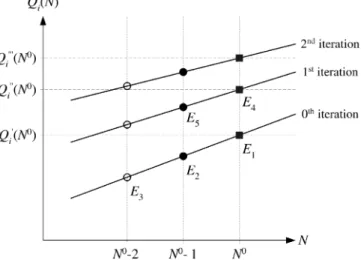
Qi N0ÿ1rÿ1s ÿ Qi N0ÿ1r ÿ þQi N0ÿ1s ÿ ÿQiÿN0; ð20Þ which is a direct consequence of (18). In addition, (20) is symmetric in r and s and scales properly with the population. A graphical representation of the fixed-point problem generated by a linear approximation function in the single-class case is shown in Fig. 1. The horizontal axis represents the population N; the vertical axis shows the queue length for stationi. Approximation (18) in this simple case is the equation of a straight line. The IMT is used according to the following strategy (see Fig. 1, N0 is the
population of interest):
Step 1. We start with estimate E1 and E2 of QiðN0Þ and
QiðN0ÿ1Þ;
Step 2.Linear interpolation based on (18) givesE3;
Step 3.The fixed-point problem (19) givesE4 andE5.
Steps 2 and 3 are repeated until values ofQiðN0Þconverge (black boxes in Fig. 1).
The approach of using trial functions with the queue lengths themselves as parameters is advantageous because it always yields fixed-point equations for the Qis. In the following, it will be used whenever possible. Approxima-tion (15) can be extended to polynomials of higher degree, so (18) will contain higher-degree Lagrangian interpolation polynomials.
Fig. 1. Representation of IMT applied to a single-class case with linear approximating function.
3.3 Another Linear Approximation (Derivation of AQL Approximation)
The AQL method is similar to the linear approximation method of Section 3.2, except that QiðNÞ=N rather than
QiðNÞis considered as linear. Equation (15) is replaced by
Qið ÞN N TiðN; PiÞ N ¼Aiþ XR r¼1 BirNr Pi¼fAi; Birg ð Þ forNnearN0: ð21Þ
If (21) is required to hold exactly at the matching populations (16), approximation (20) is replaced by
Qi N0ÿ1rÿ1s ÿ N0ÿ2 ¼ Qi N0ÿ1r ÿ N0ÿ1 þ Qi N0ÿ1s ÿ N0ÿ1 ÿ Qi N0 ÿ N0 ;
which is exactly the AQL approximation defined by (9).
3.4 The Linear Basis Expansion
More general trial functions than the ones described in the previous sections can be used. For example, one could use a Pade´ approximation (see Table 1) or, more generally, any smooth (analytic) function. In this section, we use a linear combination of independent basis functions. Let us consider J known, linearly independent, basis functions fuðNÞ and attempt a trial function
Qið Þ N TiðN; PiÞ ¼
XJ u¼1
Piufuð ÞN forNnearN0; ð22Þ with theMJparametersPiuto be determined. This choice of
TiðN;PiÞ includes both the approximation functions de-scribed above as special cases (e.g., the constant approx-imation is obtained whenJ¼1andffuðNÞg ¼ f1gand the linear approximation is obtained when J¼Rþ1 and ffuðNÞg ¼ f1;Nrg). Higher-degree polynomials may be accommodated as well. As in the previous case, it is possible to change the parameters so that the new parameters are the queue lengths themselves at some given populations, namely by specifyingJpopulation vectorsN fNð1Þ;Nð2Þ; . . . ;NðJÞgand requiring (22) to hold exactly for
these populations. ThefPitgare then specified in terms of theQiðNðvÞÞby the linear equations
Qi Nð Þv ¼X J u¼1 Piu fu Nð Þv Nð Þv 2N: ð23Þ Because they are linear, the set of equations (23) can be inverted to express thePius in terms of the queue lengths at the matching populations. We introduce the following matrix notation: P½Piu MJmatrix;unknown X½Xiv Qi Nð Þv h i MJmatrix;unknown Y½Yuv fu Nð Þv h i JJmatrix;known: ð24Þ
Equation (23) can now be rewritten asX¼PY. MatrixYis always nonsingular because the basis functions are assumed to be linearly independent. LetW ½Wvu Yÿ1. Therefore, approximation (22) becomes Qið Þ N XJ u¼1 XJ v¼1 XivWvufuð ÞN forNnearN0: ð25Þ By substituting (25) into the MVA recursion (11) and matching atNðvÞ2N, we obtain the fixed–point problem
Xiv¼ XR r¼1 Nrð ÞvLir 1þ ið ÞP J u¼1 PJ z¼1 XizWzufu Nð Þv ÿ1r PM j¼1 Ljr 1þ jð ÞP J u¼1 PJ z¼1 XjzWzufu Nð Þv ÿ1r 1vJ; ð26Þ consisting of MJequations for theMJ unknownsX. These correspond to (11) withPXand are the generalization of (19). Once the matrix ½Xiv is available, it is possible to estimateQiðNÞ for any N using (25). Note again that the ½Xiv have an immediate interpretation as queue lengths (see (24)).
The possibility exists of replacing (26) by an alternative scheme where (25) is inserted into both sides of (2) and matched at a set of J populations different from N. We recommend against this because the equations, unlike (26), are not in fixed-point form; we have not found any advantages in accuracy, providedNwas chosen reasonably.
4
I
NTERPOLATION ON“S
ERVERS”
AND“C
LASSES”
The interpolation-matching technique described in the previous section has an intrinsic limitation: It can approx-imate only the aggregate queue lengths Qi, but not the queue lengths per customer class Qir. Therefore, it can encompass algorithms like AQL, but not SB or Linearizer. In this section, we extend the formulation of the interpolation matching technique in order to approximate the Qirs individually. The extension parallels the formulation in Section 3. The basic approximation used in this case is
Qirð Þ N TirðN; PirÞ forNnearN0;
where the trial functionsTirdepend uponMRvectorsPir, each with J real elements. We specify J matching populations N fNð1Þ;Nð2Þ; . . . ;NðJÞg and impose the matching conditions Tir Nð Þu; Pir ¼ Nð Þu r Lir 1þP R s¼1 Tis Nð Þu ÿ1r; Pis PM j¼1 Ljr 1þP R s¼1 Tjs Nð Þu ÿ1r; Pjs Nð Þu 2N: ð27Þ
Equation (27) defines a set of MRJequations for the MRJ parameters. The following subsections illustrate the trial functions chosen to reproduce approximation methods corresponding to the SB and Linearizer. The more general case of linear basis functions includes all the previous ones and will be used in Section 5 to derive a new cubic approximation.
4.1 Linear Approximation Function (Derivation of Schweitzer-Bard)
We consider the linear approximation,
Qirð Þ N TirðN; PirÞ ¼AirNr forNnearN0; ð28Þ that uses MR parameters fAirg (i.e., J¼1) and R trial functions ffrðNÞg ¼ fNrg. Changing the parameters from fAirgtofQirðN0Þgand requiring that (28) holds exactly at
N0, we must have Air¼QirðN0Þ=N0r. Therefore, (28) becomes Qirð Þ N TirðN; PirÞ ¼ Qir N0 ÿ N0 r Nr forN nearN0: ð29Þ Using (29) to compute the queue length at the population vectorN0ÿ1s, we obtain Qir N0ÿ1s ÿ Qir N0 ÿ ÿrs Qir N0 ÿ N0 r ; ð30Þ which is exactly the SB approximation (5). The fixed-point problem obtained using (30) in the matching conditions (27) becomes identical to (6).
4.2 Quadratic Approximation Function (Derivation
of Linearizer)
In this section, we will show that, with a proper choice of basis functions and matching populations, the IMT is equivalent to the Linearizer approximation described in Section 2.2.3. Let us consider a quadratic expansion for the queue lengths Qirð Þ N TirðN; PirÞ ¼AirNrþ XR t¼1 BirtNrNt Pir¼fAir; Birtg ð Þ forNnearN0 ð31Þ
withMRðRþ1ÞcoefficientsPirto be determined (i.e.,MR vectors each with J¼Rþ1 real elements) and basis functions fNr;NrNsg. This approximation yields the one used by Linearizer if we take
N N0; N0ÿ1r
ð32Þ as matching populations. As before, it is possible to change the parameters by requiring (31) to hold exactly for theðRþ 1Þ populations (32)
QirðN0Þ ¼TirðN0; PirÞ
QirðN0ÿ1sÞ ¼TirðN0ÿ1s; PirÞ:
ð33Þ These conditions lead to the new trial functions
Qirð Þ N TirðN; PirÞ ¼ Nr QirðN0Þ N0 r þX R t¼1 NtÿNt0 ÿ QirðN0Þ N0 r ÿQirðN 0ÿ1 tÞ N0 r ÿrt ( ) ;
with the new parameters Pir¼ fQirðN0Þ;QirðN0ÿ1tÞg. Setting N ¼N0ÿ1sÿ1r leads to the Linearizer approx-imation (8).
4.3 The Linear Basis Expansion
The generalization of the above approximation functions is obtained by approximating the queue length Qir for any class r at a given station i with the following linear combination ofJbasis functionsfruðNÞ:
Qirð Þ N
XJ u¼1
Priufruð ÞN forNnearN0; ð34Þ wherefPriugis a set ofMRJcoefficients to be determined. As already pointed out, it is convenient to change paramet ers f rom Priu to QirðN2NÞ, whe re N fNð1Þ;Nð2Þ; . . . ;NðJÞg is a specified set of J populations (which may include N0 itself). By insisting upon equality
between the left and right sides of (34) at these populations, we obtain theMRJequations
Qir Nð Þv X J u¼1 Priufru Nð Þv Nð Þv 2N; ð35Þ which are sufficient to determine the MRJ Priu. Let’s introduce the following notation:
Pr½Priu Xr½Xriv Qir Nð Þv h i Yr½Yruv fru Nð Þv h i :
For eachr,Pr andXr are unknownMRmatrices, while Yr is a known JJ matrix. Equation (35) can then be rewritten as
Xr¼PrYr:
The Yr matrices are nonsingular if we assume the basis functions fru for each r to be linearly independent. Let Wr ½WruvYÿ 1 r , so Pr¼XrWr. Approximation (35) becomes Qirð Þ N XJ u¼1 XJ v¼1
Xriv½Wrvufruð ÞN forN nearN0: ð36Þ By substituting the above expression into the MVA recursion, we obtain the following fixed-point problem (in theMRJunknownsXr): Xriv¼ Nð Þv r Lir 1þ ið ÞP R s¼1 PJ u¼1 PJ z¼1 Xsiz½Wszufsu Nð Þv ÿ1r PM j¼1 Ljr 1þ jð ÞP R s¼1 PJ u¼1 PJ z¼1 Xsjz½Wszufsu Nð Þv ÿ1r 1vJ: ð37Þ Once theXrmatrices are available, it is possible to estimate theQirðNÞfor anyN using (36).
4.4 Generalization of the IMT Technique
The most general case of IMT uses the following approximation
where the parameters Pir enter the trial function in a nonlinearway. In all cases, the matching procedure gives a nonlinear set of equations for the parametersPir. We have two sets of equations, the interpolation equations (38):
Qir NðvÞ
Tir NðvÞ; Pir
ð39Þ and the matching equations (27)
Tir NðvÞ; Pir ¼ NðvÞ r Lir 1þ ið ÞP R s¼1 Tis NðvÞÿ1r; Pis PM j¼1 Ljr 1þ jð ÞP R s¼1 Tjs NðvÞÿ1r; Pjs : ð40Þ These are2MRJ equations for the2MRJ unknownsQir andPirand, in general, they are not in fixed-point form for thePirs. A straightforward procedure is to first solve (40) forPirand subsequently use (39) to calculateQir.
By contrast, in the previous examples, (39) was inverted explicitly to obtainPiras a function ofQirand then (40) was interpreted as a set of simultaneous equations for Qir similar to (4), (19), (26), and (37), thus obtaining a fixed-point problem for the queue lengths at the matching populations. The advantages of such an approach are:
. The first step of the strategy, inverting (39), must be executed only once when the new IMT algorithm is created, so its computational cost can be ignored;
. We obtain a fixed-point problem, which is much easier to solve than the more general equation (40);
. The unknowns of the fixed-point problem are the queue lengths, which have an immediate meaning, unlike the parametersPir.
The most important feature, however, is that the number of equations equals the number of parameters, so the matching conditions (40) serve uniquely to determine the parametersPir, even when they are not in fixed-point form. Two straightforward extensions are to let the basis func-tionsfruðNÞin (34) depend oniand let the matching points
N fNðvÞgin (35) depend oniandr. The notation becomes more complicated, but the underlying ideas remain the same. With the proposed extensions, it is also possible to treat the more general case of Pade` approximations.
5
A
NE
XAMPLE OFIMT A
PPLICATION: T
HEL
INEARIZER++ A
LGORITHMTo illustrate the ease of constructing new approximation algorithms using the IMT, we propose a cubic expression as the interpolating function for the queue lengths. The equivalence between SB and linear interpolation function and between Linearizer and quadratic interpolation func-tion has motivated the investigafunc-tion of higher order interpolation polynomial functions in order to find more accurate approximating methods. The specific form of cubic interpolation—compare with (28) and (31)—is
Qirð Þ N AirNrþ XR s¼1 BirsNrNsþ XR t¼1 XR st CirstNrNsNt Pir¼fAir; Birs; Cirstg ð Þ forN nearN0:
There are MR½ðRþ1ÞðRþ2Þ=2 unknown coefficients Pir (i.e.,MR parameter vectors each withJ¼ ðRþ1ðRþ2Þ=2
real elements). Choosing the following matching population vectors:
NnNð Þ0; Nð Þ0 ÿ1r; Nð Þ0 ÿ1rÿ1so;
leads to a new approximation method (referred to as Linearizer++) which shows much better accuracy than Linearizer. Table 2 shows the results obtained for over 4,800 randomly generated models (100 models for each specification of:M = 2, 4, 6, 8 servers, R = 2, 3 classes of customers, andN= 5, 10, 50, 100, 500, 1,000 total customers). Since queuing centers usually contribute more to the errors than delay centers do, only queuing centers have been considered in the experiments. The values of the loadings range from 0 to 100. All the parameters were selected independently and their values are uniformly distributed over their respective ranges. The table presents the average
ðeÞ, the standard deviationðeÞ, and the maximummaxðeÞ of the normalized errore of each model, defined as
e¼max i;r Qirð ÞN MVAÿQirð ÞN APP Nr ;
where QirðNÞMVA and QirðNÞAPP are the exact and
approximate solutions, respectively, for the considered model. Let us remark that the value ofe is the maximum error on the per-class customers at the servers of each model. As the table shows, the error of Linearizer++ is, on average, 1/3 of the error of Linearizer, with half the standard deviation and max error of Linearizer. In all the models, the errorseof Linearizer++ are lower then the ones of Linearizer. In general, the errors increase with the number of stations and with the number of classes.
The complexity of the three methods (SB, Linearizer, and Linearizer++) is proportional to the number of iterationsn needed to solve the fixed-point problem, and to the complexity of one iteration. The complexity of each iteration isOðM R2J3ÞwithJ¼1for SB,J¼ ðRþ1Þfor Linearizer,
andJ¼ ðRþ1ÞðRþ2Þ=2for Linearizer++. The number of iterations clearly depends on the starting point and on the termination criteria and, a priori, it may also be influenced by the number of classes, the number of stations, and the number of customers.
Fig. 2 shows the average number of iterations (and the standard deviation) as a function of the number of stations M and the number of classes R, for the three local approximation techniques. Each point in the figure is the average of 1,800 values, corresponding to 100 models, with six different numbers of customers (N= 5, 10, 50, 100, 500, 1,000) and three different approximation techniques (SB, Linearizer, Linearizer++).
An interesting result that can be drawn from the figure, is that the number of customers N and the approximate method adopted have a very limited influence on the number of iterations required for the method to converge.
On the other side, the number of iterations increases with the number of stationsMand decreases with the number of classesR.
6
D
ESIGNG
UIDELINES FORN
EWA
PPROXIMATIONT
ECHNIQUESThis section describes the guidelines for the design of new approximation techniques using IMT. Any IMT algorithm is specified by choosing:
. an integer number J (i.e., the number of unknown vector parameters), which is a dominant factor in the computational complexity of the method;
. the interpolating functions TirðN; PirÞ, with MJR parametersPir to be determined;
. the matching pointsN fNð1Þ; Nð2Þ;. . .; NðJÞg. The issues regarding each of these choices are described in the following subsections.
6.1 Choice of J
Experience suggests that good choices forJareJ¼Rþ1and
J¼ ðRþ1ÞðRþ2Þ=2 because they satisfy all three of the previously stated general rules. Note that these choices forJ are implicitly made by AQL, Linearizer, and Linearizer++.
6.2 Choice of the Interpolation Functions
The largest degree of freedom when defining a new IMT method arises with the choice of the interpolating functions. Experience suggests that:
. Choosing the trial functions to be finite-degree polynomials leads to convenient Lagrangian inter-polating polynomials and gives good insight into the interpolation method. All the known approximation methods use polynomials. Increasing the degree of the polynomial from constant to linear then to quadratic and cubic is observed to increase the method accuracy, with Linearizer++ being the most precise. However, the increase of accuracy with the increase of the polynomial degree is not expected to continue indefinitely because of the numerical instability that characterizes high degree polynomial approximations. We have observed that instability arises with a degree greater than 3. In addition, high degree polynomials are computationally unattrac-tive as the number of customer classes increases. The instability of the high degree polynomials arises because the matching population set now include points very far from N0 and such points do not contribute significantly to the accuracy of estimating
QiðN0Þ.
. It is desirable to choose the trial functionsTirðN;PirÞ such that PMi¼1TirðN; PirÞ ¼Nr is an identity (i.e., the scaling condition described in Section 2.2.1 must be verified) and similarly choose trial functions
TiðN;PiÞ such that
PM
i¼1TiðN; PiÞ ¼
PR
r¼1Nr is an identity. Inspection of (18), (29), and (31) shows that SB, Linearizer, and Linearizer++ satisfy this condi-tion and that it is straightforward to accomplish this.
. SB, Linearizer, and Linearizer++ use Lagrangian polynomials for interpolating the functions Qir=Nr rather thanQirand provide good results. A reason for this is that the functionQir=Nr is smoother than
Qir, so a low degree polynomial satisfactorily approximates it. More generally, it appears desirable to attempt interpolations on functions of the queue lengths that are known to be smoother than the
TABLE 2
Normalized Errors of Three Local Approximation Techniques
Fig. 2. Average number of iterations as a function of the number of stations and the number of classes for the three local approximation techniques.
queue lengths themselves. This is the motivation for the use of generalized Pade´ approximations.
. Other choices of trial functions besides linear basis functions (Lagrangian interpolation polynomials) have been explored. In particular, generalized Pade´ approximations appear to be both convenient and flexible. The choice of trial functions determines the ease of solving (27), which are usually not in fixed-point form.
6.3 Choice of the Matching Points
The choice of the matching pointsNðtÞhave a great impact on
the accuracy of an IMT method. Our intuition, based on the experiments performed, suggests that the matching points:
. Should be in some way “fair” to the different classes of customers;
. Should be chosen nearN0: IMT methods are local, thus they provide good results locally (i.e., at points nearN0);
. Should be below N0 (i.e., for networks with fewer
customers than N0) because of the well-known property of the upward MVA recursion to smooth errors [8];
. Should constitute a “compact” set, without gaps in it (see the following section).
A good choice of matching points is N N0; N0ÿ1r
;
which is the choice made by Linearizer and AQL, or N Nð Þ0; Nð Þ0 ÿ1r; Nð Þ0 ÿ1rÿ1s
n o
;
which is the choice made by Linearizer++. Good choices of the matching points are
N¼Wð Þ v N j NrNr08r
ÿ
^ ðN N0ÿvÞ
; ð41Þ where vrefers to the maximum distance from N0. Let us remark that all the points contained in the set WðvÞ influence QiðN0Þ in the MVA recursion. We refer to such set of points as thewake setfor the pointN0. Fig. 3 shows the wake set for a two-class network with v¼3.
6.3.1 Characteristics of the Matching Population Set
W e f o u n d g o o d r e s u l t s i f o u r c h o i c e o f N¼ fNð1Þ;Nð2Þ; . . . ;NðJÞgmet three criteria:
1. N02N;
2. EachNðuÞlies in the wake set ofN0;
3. EachNðuÞlies in the wake set of other numbersNðvÞ. The explanation is that the interpolation formula QiðNÞ ¼
TiðN;PiÞ is implicitly assumed to hold perfectly atall the points fNð1Þ;Nð1Þÿ1r;Nð2Þ;Nð2Þÿ1r; . . .g 8r. This is too much to expect. Compare, for example, Fig. 1 and Fig. 4, both showing a graphical representation of linear approx-imation (15) with a single (R¼1) and two parameters (J¼2). Fig. 4 shows the most general (and worst) choice of matching population set. Starting with estimateE1andE2
of the queue lengths at populations Nð1Þ and Nð2Þ, linear interpolation givesE3andE4, which are used to iterate the
method. Linear interpolation also givesE0, which is used to
test the method convergence. One is therefore attempting, in the worst case, to fit a straight line through five points fNð0Þ;Nð1Þ;Nð1Þÿ1;Nð2Þ;Nð2Þÿ1g. One of these five points
is eliminated by rule 1 and another by rules 2 and 3. The result is to have to fit a straight line through three points fNð0Þ;Nð0Þÿ1;Nð0Þÿ2g, a task which is much more likely
to succeed, as shown in Fig. 1.
7
C
ONCLUSIONSIn this paper, we have presented an interpolation-matching technique that provides an analytical framework under which all the known local approximation techniques for the solution of closed product-form queuing networks can be described and analyzed.
We have identified the characteristics and the para-meters of approximating methods that impact on their complexity and accuracy. In particular, we have shown that differences in the accuracy are related to the specific forms of the corresponding interpolating functions. As an example of the power of the IMT technique, throughout its application, we have constructed a new algorithm that exhibits better accuracy results than previous ones.
Fig. 3. The “wake set” in a two-class network.
Fig. 4. Graphical representation of IMT applied at a simple single-class case with a linear approximating function and a generic matching population set.
Guidelines are given for the construction of new approx-imation techniques with different accuracy and computa-tional complexity by properly selecting the matching points and the interpolating functions.
Our current investigation focuses on choosing noninte-ger populations in order to be closer to target population; on choosing the function parameters to locally match both functions and derivatives of the MVA recursion or to do a least squares fit over a prescribed range of populations; on choosing the trial functions and extending the results to load-dependent servers.
A
PPENDIXThis appendix shows how to obtain a fixed–point problem for the parametersfAir;Birgfrom the linear approximation defined in Section 3.2: Qið Þ N TiðN; PiÞ ¼Aiþ XR r¼1 BirNrðPi¼fAi; BirgÞ; forN nearN0; ð42Þ
when using the matching points NN0; N0ÿ1r :
If, for each N2N, we write the matching condition (11) together with the approximation (42), we obtain the following equations: Aiþ XR r¼1 BirNr0¼ XR s¼1 N0 sLis 1þ ið Þ AiþP R r¼1 BirÿNr0ÿrs PM j¼1 Ljs 1þ jð Þ AjþP R r¼1 Bjr Nr0ÿrs ÿ ð43Þ Aiþ XR r¼1 Bir Nr0ÿrt ÿ ¼ XR s¼1 N0 sÿst ÿ Lis 1þ ið Þ AiþP R r¼1 Bir Nr0ÿrsÿrt ÿ PM j¼1 Ljs 1þ jð Þ AjþP R r¼1 Bjr Nr0ÿrsÿrt ÿ : ð44Þ These areMðRþ1Þ equations for theMðRþ1Þunknowns fAi;Birg. They are neither linear nor in fixed-point form. The fixed-point form can be obtained by adding and subtracting (43) and (44): Ai¼P R s¼1 N0 sLis 1þ ið Þ AiþP R r¼1 BirðN0rÿrsÞ PM j¼1 Ljs 1þ jð Þ AjþP R r¼1 BjrðNr0ÿrsÞ ÿP R r¼1 BirNr0 Bit¼P R s¼1 N0 sÿst ð ÞLis 1þ ið Þ AiþP R r¼1 BirðN0rÿrsÿrtÞ PM j¼1 Ljs 1þ jð Þ AjþP R r¼1 BjrðN0rÿrsÿrtÞ þ ÿPR s¼1 N0 sLis 1þ ið Þ AiþP R r¼1 BirðNr0ÿrsÞ PM j¼1 Ljs 1þ jð Þ AjþP R r¼1 BjrðNr0ÿrsÞ : 8 > > > > > > > > > > > > > > > > > > > < > > > > > > > > > > > > > > > > > > > : ð45Þ
Successive substitutions on this set of equations will presumably converge to the parametersfAi;Birgand then (15) will produce an estimate ofQiðNÞ.
A
CKNOWLEDGMENTSThis work was supported in part by the MIUR COFIN 2001 project. The authors would like to thank Francesco Schiavoni for his contribution to this work and the reviewers for their helpful comments.
R
EFERENCES[1] G.A. Baker and P. Graves-Morris, “Pade´ Approximations,” Encyclopedia of Math. and Its Applications, second ed., vol. 59, Cambridge, U.K.: Cambridge Univ. Press, 1996.
[2] Y. Bard, “Some Extensions to Multiclass Queueing Network Analysis,” Proc. Fourth Int’l Symp. Modeling and Performance Evaluation of Computer Systems, A. Butrimenko M. Arato, and E. Gelenbe, eds., pp. 51-62, 1979.
[3] F. Baskett, K.M. Chandy, R.R. Muntz, and R. Palacios, “Open, Closed and Mixed Networks of Queues with Different Classes of Customers,”J. ACM,vol. 22, no. 2, pp. 248-260, 1975.
[4] J.P. Buzen, “Computational Algorithms for Closed Queueing Networks with Exponential Servers,”Comm. ACM,vol. 16, no. 9, pp. 527-531, 1973.
[5] W.M. Chow, “Approximations for Large Scale Closed Queueing Networks,”Performance Evaluation,vol. 3, no. 1, pp. 1-12, 1983.
[6] K.M. Chandy and D. Neuse, “Linearizer: A Heuristic Algorithm for Queueing Network Models of Computing Systems,” Comm. ACM,vol. 25, no. 2, pp. 126-134, 1982.
[7] D.L. Eager and K.C. Sevcik, “Performance Bound Hierarchies for Queueing Networks,”ACM Trans. Computer Systems,vol. 1, no. 2, pp. 99-115, 1983.
[8] D.L. Eager and K.C. Sevcik, “Bound Hierarchies for Multiple-Class Queueing Networks,”J. ACM,vol. 33, no. 4, pp. 179-206, 1986.
[9] M. Reiser and S. Lavenberg, “Mean-Value Analysis of Closed Multichain Queueing Networks,”J. ACM,vol. 27, no. 2, pp. 313-322, 1980.
[10] M. Reiser and H. Kobayashi, “Queueing Networks with Multiple Closed Chains: Theory and Computational Algorithms,”IBM J. Research and Development,vol. 19, pp. 283-294, 1975.
[11] P.J. Schweitzer, “Approximate Analysis of Multiclass Closed Queueing Networks of Queues,”Proc. Int’l Conf. Stochastic Control and Optimization,Apr. 1979.
[12] P.J. Schweitzer, “A Survey of Mean Value Analysis, Its General-izations, and Applications, for Networks of Queues,”Proc. Second Int’l Workshop Netherlands Nat’l Network for the Math. on Operations Research,Feb. 1991.
[13] E. de Souza e Silva and R.R. Muntz, “A Note on the Computa-tional Cost of the Linearizer Algorithm,”IEEE Trans. Computers, vol. 39, no. 6, pp. 840-842, June 1990.
[14] J.R. Spirn, “Queueing Networks with Random Selection for Service,”IEEE Trans. Software Eng.,vol. 3, no. 1, pp. 287-289, 1979.
[15] J. Zahorjan, D.L. Eager, and H.M. Sweillam, “Accuracy, Speed and Convergence of Approximate Mean Value Analysis,”Performance Evaluation,vol. 8, no. 4, pp. 255-270, 1988.
[16] H. Wang and K.C. Sevcik, “Experiences with Improved Approx-imate Mean Value Analysis Algorithms,” Proc. 10th Int’l Conf. Modeling Techniques and Tools, R. Puigjaner, N.N. Savino, and B. Serra, eds., pp. 280-291, 1998.
[17] P. Cremonesi, F. Schiavoni, P.J. Schweitzer, and G. Serazzi, “An Interpolation-Matching Framework for the Approximate Solution of Closed Multiclass Queuing Networks,” Internal Report N 27/ 1997, Dipartimento di Elettronica e Informazione, Politecnico di Milano, 1997.
Paolo Cremonesireceived the MSc degree in aerospace engineering in 1992 and the PhD degree in computer science in 1996, both from the Politecnico di Milano, Milan, Italy. He is currently an assistant professor of computer science with the Politecnico di Milano. His current research interests include high-perfor-mance computing modeling and other topics related to the performance evaluation of com-puter systems and networks.
Paul J. Schweitzeris a professor of business administration at the W.E. Simon Graduate School of Business Administration at the Uni-versity of Rochester, New York, where he teaches in the general areas of information technology, stochastic processes, management science, and operations management. His cur-rent research areas include Markovian decision processes and iterative aggregation theory. He has worked in the field of performance evalua-tion for more than 30 years and is the inventor of approximate Mean Value Analysis, the topic of this paper.
Giuseppe Serazzireceived the Laurea degree in mathematics from the University of Pavia, Italy, in 1969. He is a professor in the Computer Science Department at the Politecnico di Milano, Milano, Italy. He spent four years with the University of Milano before joining the Politecni-co in 1991. From 1978 to 1987, he was an associate professor in the Department of Mathe-matics, University of Pavia. His current research interests include modeling and other topics related to performance evaluation of computer systems, Web servers, intranets, Internet, and high-performance computing. He is a member of the IEEE Computer Society.
.For more information on this or any computing topic, please visit our Digital Library athttp://computer/org/publications/dlib.