ScholarlyCommons
Statistics Papers
Wharton Faculty Research
2-2016
Estimating Structured High-Dimensional
Covariance and Precision Matrices: Optimal Rates
and Adaptive Estimation
Tony Cai
University of PennsylvaniaZhao Ren
University of PittsburghHarrison H. Zhou
Yale UniversityFollow this and additional works at:
http://repository.upenn.edu/statistics_papers
Part of the
Physical Sciences and Mathematics Commons
This paper is posted at ScholarlyCommons.http://repository.upenn.edu/statistics_papers/78
For more information, please [email protected].
Recommended Citation
Cai, T., Ren, Z., & Zhou, H. H. (2016). Estimating Structured High-Dimensional Covariance and Precision Matrices: Optimal Rates and Adaptive Estimation.Electronic Journal of Statistics, 10(1), 1-59.http://dx.doi.org/10.1214/15-EJS1081
Estimating Structured High-Dimensional Covariance and Precision
Matrices: Optimal Rates and Adaptive Estimation
Abstract
This is an expository paper that reviews recent developments on optimal estimation of structured
high-dimensional covariance and precision matrices. Minimax rates of convergence for estimating several classes of
structured covariance and precision matrices, including bandable, Toeplitz, sparse, and sparse spiked
covariance matrices as well as sparse precision matrices, are given under the spectral norm loss. Data-driven
adaptive procedures for estimating various classes of matrices are presented. Some key technical tools
including large deviation results and minimax lower bound arguments that are used in the theoretical analyses
are discussed. In addition, estimation under other losses and a few related problems such as Gaussian
graphical models, sparse principal component analysis, factor models, and hypothesis testing on the
covariance structure are considered. Some open problems on estimating high-dimensional covariance and
precision matrices and their functionals are also discussed.
Keywords
Adaptive estimation, banding, block thresholding, covariance matrix, factor model, Frobenius norm, Gaussian
graphical model, hypothesis testing, minimax lower bound, operator norm, optimal rate of convergence,
precision matrix, Schatten norm, spectral norm, tapering, thresholding
Disciplines
Physical Sciences and Mathematics
Vol. 10 (2016) 1–59 ISSN: 1935-7524
DOI:10.1214/15-EJS1081
Estimating structured high-dimensional
covariance and precision matrices:
Optimal rates and adaptive estimation
∗
T. Tony Cai†
Department of Statistics, The Wharton School, University of Pennsylvania, Philadelphia, PA 19104, USA
e-mail:[email protected]
Zhao Ren
Department of Statistics, University of Pittsburgh, Pittsburgh, PA 15260, USA e-mail:[email protected]
and
Harrison H. Zhou‡
Department of Statistics, Yale University, New Haven, CT 06511, USA e-mail:[email protected]
Abstract: This is an expository paper that reviews recent developments on optimal estimation of structured high-dimensional covariance and preci-sion matrices. Minimax rates of convergence for estimating several classes of structured covariance and precision matrices, including bandable, Toeplitz, sparse, and sparse spiked covariance matrices as well as sparse precision matrices, are given under the spectral norm loss. Data-driven adaptive procedures for estimating various classes of matrices are presented. Some key technical tools including large deviation results and minimax lower bound arguments that are used in the theoretical analyses are discussed. In addition, estimation under other losses and a few related problems such as Gaussian graphical models, sparse principal component analysis, factor models, and hypothesis testing on the covariance structure are considered. Some open problems on estimating high-dimensional covariance and preci-sion matrices and their functionals are also discussed.
MSC 2010 subject classifications:Primary 62H12; secondary62F12, 62G09.
Keywords and phrases:Adaptive estimation, banding, block threshold-ing, covariance matrix, factor model, Frobenius norm, Gaussian graphical model, hypothesis testing, minimax lower bound, operator norm, optimal rate of convergence, precision matrix, Schatten norm, spectral norm, taper-ing, thresholding.
Received August 2014.
∗Discussed in 10.1214/15-EJS1018, 10.1214/15-EJS1081A, 10.1214/15-EJS1006 and 10.1214/15-EJS1019; rejoinder at10.1214/15-EJS1081REJ.
†The research of Tony Cai was supported in part by NSF Grant DMS-1208982 and NIH
Grant R01 CA 127334-05.
‡The research of Harrison Zhou was supported in part by NSF Grant DMS-1209191.
Contents
1 Introduction . . . 2
1.1 Estimation of structured covariance matrices . . . 6
1.2 Estimation of structured precision matrices . . . 11
1.3 Organization of the paper . . . 12
2 Estimation of structured covariance matrices . . . 13
2.1 Bandable covariance matrices . . . 13
2.2 Toeplitz covariance matrices . . . 17
2.3 Sparse covariance matrices . . . 18
2.4 Spiked sparse covariance matrices . . . 21
3 Minimax upper bounds of estimating sparse precision structure . . . . 26
3.1 Sparse precision matrix: Adaptive minimax upper bound under spectral norm . . . 27
3.2 Individual entries of sparse precision matrix: Asymptotic normality 29 3.3 Related results . . . 31
3.4 Computational issues . . . 33
4 Lower bounds . . . 34
4.1 General minimax lower bound techniques . . . 34
4.2 Application of Assouad’s lemma to estimating bandable covari-ance matrices . . . 37
4.3 Application of Le Cam’s method to estimating entries of precision matrices . . . 38
4.4 Application of Le Cam-Assouad’s method to estimating sparse precision matrices . . . 40
4.5 Application of Fano’s lemma to estimating toeplitz covariance matrices . . . 42
5 Discussions . . . 43
5.1 Non-centered case . . . 43
5.2 Positive (semi-)definiteness . . . 44
5.3 Hypothesis testing for the covariance structure . . . 45
6 Some open problems . . . 48
6.1 Optimality for covariance matrix estimation under Schattenqnorm 48 6.2 Lower Bound via packing number . . . 49
6.3 Optimal estimation of matrix functionals . . . 49
References . . . 50
1. Introduction
Driven by a wide range of applications in many fields, from medicine to signal processing to climate studies and social science, high-dimensional statistical inference has emerged as one of the most important and active areas of current research in statistics. There have been tremendous recent efforts to develop new methodologies and theories for the analysis of high-dimensional data, whose dimension p can be much larger than the sample size n. The methodological
and theoretical developments in high-dimensional statistics are mainly driven by the important scientific applications, but also by the fact that some of these high-dimensional problems exhibit new features that are very distinct from those in the classical low-dimensional settings.
Covariance structure plays a particularly important role in high-dimensional data analysis. A large collection of fundamental statistical methods, including the principal component analysis, linear and quadratic discriminant analysis, clustering analysis, and regression analysis, require the knowledge of the ance structure or some aspects thereof. Estimating a high-dimensional covari-ance matrix and its inverse, the precision matrix, is becoming a crucial problem in many applications including functional magnetic resonance imaging, analysis of gene expression arrays, risk management and portfolio allocation.
The standard and most natural estimator, the sample covariance matrix, performs poorly and can lead to invalid conclusions in the high-dimensional set-tings. For example, whenp/n→c∈(0,∞], the largest eigenvalue of the sample covariance matrix is not a consistent estimate of the largest eigenvalue of the population covariance matrix, and the eigenvectors of the sample covariance matrix can be nearly orthogonal to the truth. See Wachter (1976,1978), John-stone (2001), El Karoui (2003), Paul (2007), and Johnstone and Lu (2009). In particular, whenp > n, the sample covariance matrix is not invertible, and thus cannot be applied in many applications that require estimation of the precision matrix.
To overcome the difficulty due to the high-dimensionality, structural assump-tions are needed in order to estimate the covariance or precision matrix con-sistently. Various families of structured covariance and precision matrices have been introduced in recent years, including bandable covariance matrices, sparse covariance matrices, spiked covariance matrices, covariances with a tensor prod-uct strprod-ucture, sparse precision matrices, bandable precision matrix via Cholesky decomposition, and latent graphical models. These different structural assump-tions are motivated by various scientific applicaassump-tions, such as genomics, genetics, and financial economics. Many regularization methods have been developed ac-cordingly to exploit the structural assumptions for estimation of covariance and precision matrices. These include the banding method in Wu and Pourahmadi (2009) and Bickel and Levina (2008a), tapering in Furrer and Bengtsson (2007) and Cai et al. (2010), thresholding in Bickel and Levina (2008b), El Karoui (2008) and Cai and Liu (2011a), penalized likelihood estimation in Huang et al. (2006), Yuan and Lin (2007), d’Aspremont et al. (2008), Banerjee et al. (2008), Rothman et al. (2008), Lam and Fan (2009), Ravikumar et al. (2011), and Chandrasekaran et al. (2012), regularizing principal components in Johnstone and Lu (2009), Zou et al. (2006), Cai, Ma, and Wu (2013), and Vu and Lei (2013), and penalized regression for precision matrix estimation in Meinshausen and B¨uhlmann (2006), Yuan (2010), Cai et al. (2011), Sun and Zhang (2013), and Ren et al. (2015).
Parallel to methodological advances on estimation of covariance and preci-sion matrices there have been theoretical studies of the fundamental difficulty of the various estimation problems in terms of the minimax risks. Cai et al.
(2010) established the optimal rates of convergence for estimating a class of high-dimensional bandable covariance matrices under the spectral norm and Frobenius norm losses. Rate-sharp minimax lower bounds were obtained and a class of tapering estimators were constructed and shown to achieve the optimal rates. Cai and Zhou (2012a,b) considered the problems of optimal estimation of sparse covariance and sparse precision matrices under a range of losses, includ-ing the spectral norm and matrix 1 norm losses. Cai, Ren, and Zhou (2013) studied optimal estimation of a Toeplitz covariance matrix by using a method inspired by an asymptotic equivalence theory between the spectral density esti-mation and Gaussian white noise established in Golubev et al. (2010). Cai et al. (2015) solved the minimax estimation problem for a large class of sparse spiked covariance matrices under the spectral norm loss. Recently Ren et al. (2015) obtained fundamental limits on estimation of individual entries of a sparse pre-cision matrix.
Standard techniques often fail to yield good results for many of these matrix estimation problems, and new tools are thus needed. In particular, for estimating sparse covariance matrices under the spectral norm, a new lower bound tech-nique was developed in Cai and Zhou (2012b) that is particularly well suited to treat the “two-directional” nature of the covariance matrices, where one direc-tion is along the rows and another along the columns. The result can be viewed as a generalization of Le Cam’s method in one direction and Assouad’s lemma in another. This new technical tool is useful for a range of other estimation problems. For example, it was used in Cai et al. (2012) for establishing the opti-mal rate of convergence for estimating sparse precision matrices and Tao et al. (2013) applied the technique to obtain the optimal rate for volatility matrix estimation.
The goal of the present paper is to provide a survey of these recent optimal-ity results on estimation of structured high-dimensional covariance and precision matrices, and discuss some key technical tools that are used in the theoretical analyses. In addition, we will present data-driven adaptive procedures for es-timation of various structured matrices. The main focus is on the bandable, Toeplitz, sparse, and sparse spiked covariance matrices as well as sparse pre-cision matrices. Among these classes of matrices, the optimal procedures for estimating the bandable, Toeplitz, and sparse covariance matrices are obtained by “smoothing” or thresholding the sample covariance matrices based on var-ious sparsity assumptions. In contrast, estimation of sparse spiked covariance matrices, which have sparse principal components, requires significantly differ-ent techniques to achieve optimality results. A few related problems such as sparse principal component analysis, factor models, and hypothesis testing on the covariance structure are also considered. Some open problems will be dis-cussed at the end.
Throughout the paper, we assume that we observe a random sample{X(1), . . . , X(n)} which consists of n independent copies of ap-dimensional random vec-torX = (X1, . . . , Xp) following some distribution with covariance matrix Σ = (σij). The goal is to estimate the covariance matrix Σ and its inverse, the pre-cision matrix Ω = Σ−1= (ωij), based on the sample
ease of presentation we assumeE(X) = 0. This assumption is not essential. The non-centered mean case will be briefly discussed in Section 5.
Notations.Before we present a concise summary of the optimality results for estimating various structured covariance and precision matrices in this section, we introduce some basic notation that will be used in the rest of the paper. For any vectorx∈Rp, we use||x||
ωto denote its ωnorm with the convention that ||x|| = ||x||2. For any p by q matrix M = (mij) ∈ Rp×q, we use M to denote its transpose. The matrix ω operator norm is denoted by ||M||ω =
max||x||ω=1||M x||ω with the convention||M|| =||M||2 for the spectral norm. Moreover, the entrywiseωnorm, that is, theωnorm ofM viewed as a vector, is denoted by||M||ωand the Frobenius norm is represented by||M||F =||M||2= (i,jm2
ij)1/2. The submatrix with rows indexed byI and columns indexed by
J is denoted by MI,J. When the submatrix is a vector or a real number, we sometimes also use the lower case minstead ofM. We use||f||∞= supx|f(x)| to denote the sup-norm of a function f(·), and I{A} to denote the indicator function of an eventA. We denote the covariance matrix of a random vectorX
by Cov(X) with the convention Var(X) = Cov(X) whenX is a random variable. For a symmetric matrix M,M 0 means positive definiteness,M 0 means positive semi-definiteness and det(M) is its determinant. We use λmax(M) and
λmin(M) to denote its largest and smallest eigenvalues respectively. Given two sequences an and bn, we write an = O(bn), if there is some constant C > 0 such that an≤Cbn for alln, and an=o(bn) impliesan/bn→0. The notation
an bnmeansan =O(bn) andbn=O(an). Then×pdimensional data matrix is denoted by X = (X(1), . . . , X(n)) and the sample covariance matrix with known E(X) = 0 is then defined as ˆΣn =XX/n = (ˆσij). For any index set
I ⊆ {1, . . . , p}, we denote byXI the submatrix ofXconsisting of the columns ofXindexed byI. The following definition of sub-Gaussian distributions is used throughout the paper.
Definition 1. The distribution of a random vectorXis said to be sub-Gaussian with constant ρ >0 if
P{|v(X−EX)|> t} ≤2e−t2ρ/2,
for allt >0 and all deterministic unit vectors v= 1.
Several matrix norms are used for the loss functions and in the technical analysis. These include the spectral norm·, matrix1 operator norm|| · ||1, matrix ∞ operator norm || · ||∞ and Frobenius norm || · ||F among others. In particular, for symmetric matrices, the spectral norm is the largest singular value. The matrix1(∞) operator norms are the largest column (row) sum of absolute values. Hence for symmetric matrices, these two norms coincide with each other. While the choice of the loss function varies according to specific applications and needs, the minimax behavior of the matrix estimation critically depends on the norm under which the error is measured. Matrix estimation under the Frobenius norm loss is essentially a vector estimation problem. What
really makes matrix estimation apart from it is those estimation problems under matrix operator norm losses, which are highly non-additive with respect to entries of the matrix. In particular, estimating covariance and precision matrices under the spectral norm loss brings in many new challenges as well as insights. We present the optimality results in the rest of this section under the Gaussian assumption with the focus on estimation under the spectral norm loss. More general settings will be discussed in Sections 2 and 3. A brief discussion on estimation under the Schattenqnorm losses is given in Section6.
1.1. Estimation of structured covariance matrices
We will consider in this paper optimal estimation of a range of structured covari-ance matrices, including bandable, Toeplitz, sparse and sparse spiked covaricovari-ance matrices.
Bandable covariance matrices
The bandable covariance structure exhibits a natural “order” or “distance” among variables. This assumption is mainly motivated by time series with many scientific applications such as climatology and spectroscopy. See, for example, Friston et al. (1994) and Visser and Molenaar (1995). We consider settings where
σij is close to zero when |i−j| is large. In other words, the variablesXi and
Xj are nearly uncorrelated when the distance|i−j|between them is large. The following parameter space was proposed in Bickel and Levina (2008a) (see also Wu and Pourahmadi (2003)), Fα(M0, M) = Σ : max j i
{|σij|:|i−j|> k} ≤M k−αfor allk, andλmax(Σ)≤M0
.
(1) The parameterαspecifies how fast the sequenceσijdecays to zero asj→ ∞for each fixedi. This can be viewed as the smoothness parameter of the classFα, which is usually seen in nonparametric function estimation problems. In partic-ular, for stationary processes, the parameter αis related to the smoothness of the corresponding spectral density function, which makes Fα(M0, M) a natu-ral class of covariance matrices. See Grenander and Szeg¨o (1958) for details. A largerαimplies a smaller number of “effective” parameters in the model. Some other classes of bandable covariance matrices have also been considered in the literature, for example,
Gα(M1) =
Σp×p:|σij| ≤M1(|i−j|+ 1)−α−1
. (2)
Note that Gα(M1) ⊂ Fα(M0, M) if M0 and M are sufficiently large. We will mainly focus on the larger class (1) in this paper. Assume that p ≤ exp(n)
for some constant > 0, then the optimal rate of convergence for estimating the covariance matrix under the spectral norm loss over the class Fα(M0, M) is given as follows. See Cai et al. (2010).
Theorem 1(Bandable Covariance Matrix). SupposeX is Gaussian. The min-imax risk of estimating the covariance matrix over the bandable class given in (1) under the spectral norm loss is
inf ˆ Σ sup Fα(M0,M) EΣˆ −Σ2 min logp n +n − 2α 2α+1 , p n .
The minimax upper bound is derived by using a tapering estimator and the key raten−2α2α+1 in the minimax lower bound is obtained by applying Assouad’s lemma. We will discuss the important technical details in Sections 2.1and 4.2 respectively. An adaptive block thresholding procedure, not depending on the knowledge of smoothness parameter α, is also introduced in Section2.1.
Toeplitz covariance matrices
Toeplitz covariance matrix arises naturally in the analysis of stationary stochas-tic processes with a wide range of applications in many fields, including engi-neering, economics, and biology. See, for instance, Franaszczuk et al. (1985), Fuhrmann (1991) and Quah (2000) for specific applications. It can also be viewed as a special case of bandable covariance matrices. Similar decay or smoothness assumption like the one given in (1) is imposed, but each descending diago-nal from left to right is constant for a Toeplitz matrix. Specifically, suppose the random vector X = (X1, . . . , Xp) consists of the first p variables of a fixed zero mean stationary process {Xi} as p → ∞. Then the Toeplitz co-variance matrix Σ of X is uniquely determined by the autocovariance sequence (σm)≡(σ0, σ1, . . . , σp−1, . . .) of{Xi} withσij =σ|i−j|=E(XiXj).
It is well known that the spectrum of Toeplitz covariance matrix Σ is closely connected to the spectral density of the stationary process {Xi}given by
f(x) = (2π)−1 σ0+ 2 ∞ m=1 σmcos (mx) , forx∈[−π, π].
See, e.g., Grenander and Szeg¨o (1958). Motivated by time series applications, we consider the following class of Toeplitz covariance matrices FTα(M0, M) defined in terms of the smoothness of the spectral densityf. Letα=γ+β >0, where γis the largest integer strictly less thanα, 0< β≤1,
FTα(M0, M) = f :f∞≤M0 and f(γ)(·+h)−f(γ)(·) ∞≤M h β. (3) In other words, the parameter space FTα(M0, M) contains the Toeplitz co-variance matrices whose corresponding spectral density functions are of H¨older
smoothness α. See, e.g., Parzen (1957) and Samarov (1977). Another parame-ter space, which directly specifies the decay rate of the autocovariance sequence (σm), has also been considered in the literature, see, Cai, Ren, and Zhou (2013). Under the assumption (np/log(np))2α1+1 < p/2, the following theorem gives the optimal rate of convergence for estimating the Toeplitz covariance matrices over the classFTα(M0, M) under the spectral norm loss.
Theorem 2 (Toeplitz Covariance Matrix). SupposeX is Gaussian. The mini-max risk of estimating the Toeplitz covariance matrices over the class given in (3) satisfies inf ˆ Σ sup FTα(M0,M) EΣˆ −Σ2 log(np) np 2α 2α+1 .
The minimax upper bound is attained by a tapering procedure on certain estimators of autocovariance sequence, which is different from those banding estimators considered in Bickel and Levina (2008a) or Furrer and Bengtsson (2007). The minimax lower bound is established through the construction of a more informative model and an application of Fano’s lemma. The essential technical details can be found in Sections2.2and4.5respectively. See Cai, Ren, and Zhou (2013) for further details.
Sparse covariance matrices
For estimating bandable and Toeplitz covariance matrices, one can take advan-tage of the information from the natural “order” on the variables. However, in many other applications such as genomics, there is no knowledge of distance or metric between variables, but the covariance between most pairs of the variables are often assumed to be insignificant. The class of sparse covariance matrices assumes that most of entries in each row and each column of the covariance matrix are zero or negligible. Compared to the previous two classes, there is no information on the “order” among the variables. We consider the following large class of sparse covariance matrices,
H(cn,p) = Σ : max 1≤i≤p p j=1 min{(σiiσjj)1/2, | σij| (logp)/n} ≤cn,p . (4) If an extra assumption that the variances σii are uniformly bounded with maxiσii≤ρfor some constantρ >0 is imposed, thenH(cn,p) can be defined in terms of the maximal truncated1norm max1≤i≤p
p
j=1min{1,|σij|(n/logp)1/2}, which has been considered in high-dimensional regression setting (see, for ex-ample, Zhang and Zhang (2012)).
For recovering the support of the sparse covariance matrices, it is natural to consider the following parameter space in which there are at mostcn,p nonzero entries in each row/column of a covariance matrix,
H0(cn,p) = Σ : max 1≤i≤p p j=1 I{σij = 0} ≤cn,p . (5)
One important feature of the classes H(cn,p) and H0(cn,p) is that they do not put any constraint on the variances σii, i = 1, . . . , p. Therefore the vari-ances σii can be in a very wide range and possibly maxiσii → ∞. When the additional bounded variance condition maxiσii ≤ ρ for some constant ρ >0 is imposed, it can be shown that the class H(cn,p) contains other commonly considered classes of sparse covariance matrices in the literature, including an
q ball assumption maxi
p
j=1|σij|q ≤sn,p in Bickel and Levina (2008b), and a weak q ball assumption max1≤j≤pσj[k]
q
≤ sn,p/k for each integer k in Cai and Zhou (2012a) where σj[k] is the kth largest entry in magnitude of the jth row (σij)1≤i≤p. More specifically, these two classes of sparse covari-ance matrices are contained inH(cn,p) withcn,p=Cqsn,p(n/logp)q/2for some constant Cq depending on q only. The class H(cn,p) also covers the adaptive sparse covariance classUq∗(sn,p) proposed in Cai and Liu (2011a), in which each row/column (σij)1≤i≤p is assumed to be in a weightedq ball for 0≤q <1,i.e., maxi
p
j=1(σiiσjj)(1−q)/2|σij|q≤sn,p. SimilarlyUq∗(sn,p)⊂ H(cn,p) withcn,p=
Cqsn,p(n/logp)q/2 for 0≤q <1. Although the class H(cn,p) is slightly larger than the classes defined viaq ball, weakq ball under bounded variances condi-tion and the classUq∗(sn,p), the minimax risks of estimation over these different classes are the same. Indeed, the least favorable subclass of H(cn,p) chosen to establish the minimax lower bound is contained in other smaller classes. See Cai and Zhou (2012b) for further details on the minimax lower bound construc-tion. It is worthwhile to point out that the class H(cn,p) is less general than the ones considered in El Karoui (2008) for which consistency results under the spectral norm loss were established. We advocate the larger sparse covari-ance class H(cn,p) in this paper not only because it contains almost all other classes considered in the literature, but also the comparison between the noise level ((σiiσjjlogp)/n)1/2 and the signal level |σij| captures the essence of the sparsity of the model.
Under some mild conditions 1≤cn,p≤C
n/(logp)3 and p≥nφ for some constants φ and C >0, the optimal rate of convergence for estimating sparse covariance matrices over the class H(cn,p) under the spectral norm is given as follows. See Cai and Zhou (2012b).
Theorem 3(Sparse Covariance Matrix). SupposeXis Gaussian. The minimax risk of estimating a sparse covariance matrix over the classH(cn,p)given in (4) satisfies inf ˆ Σ sup H(cn,p) EΣˆ −Σ2 c2 n,p logp n .
The distributional assumption onX can be significantly relaxed. See Section 2.3for further details. Besides, an adaptive thresholding estimator is constructed in Section2.3, and it is shown to be adaptive to the variability of the individual entries and attains the minimax upper bound. The lower bound argument for estimation under the spectral norm was given in Cai and Zhou (2012b) by applying Le Cam-Assouad’s method, which is introduced in Section4.1.
Sparse spiked covariance matrices Spiked covariance matrix
Σ = r
i=1
λrvivi+I, (6)
where λ1 ≥ λ2 ≥ · · · ≥ λr > 0 and the vectors v1, . . . , vr are orthonormal, arises naturally in principal component analysis as well as factor models with homoscedastic noise. In particular, the firstreigenvalues of Σ are strictly larger than 1, the remaining eigenvalues. Since the spectrum of Σ hasrspikes, (6) was first named spiked covariance model in Johnstone (2001).
Before defining the sparse spiked covariance structure, we introduce some notation. Let the set ofpbyrmatrices with orthonormal columns beO(p, r) =
{V ∈Rp×r:VV =I}. For any suchV = (v
1, v2, . . . , vr)∈O(p, r), we denote itsith row byVi,∗. The diagonal matrix Λ = diag(λ1, . . . , λr). The class of sparse spiked covariance matrices imposes the sparsity on the rows ofV. Specifically, we define J(cn,p, rn,p, λn,p)= Σ =VΛV+I: 0< λr≤ · · · ≤λ1≤λn,p, V ∈O(p, r),pj=1I{Vj,∗=0} ≤cn,p , (7) where 1 ≤ rn,p ≤ cn,p ≤ p. More concretely, the group-sparse structure is imposed on therleading eigenvectors of Σ inJ(cn,p, rn,p, λn,p) and the number of nonzero rows of V is no more than cn,p. As a consequence, as the sum of a sparse matrix and an identity matrix, the covariance matrix Σ itself is also sparse. In particular, there are no more than cn,p nonzero entries in each row and each column of Σ and henceJ(cn,p, rn,p, λn,p)⊂ H0(cn,p) defined in (5). However, compared with the previous three structures, sparse spiked covariance matrix has a very different structural component, the rankrmatrixri=1λrvivi. This extra low-rank structure, together with the sparsity assumption yields a faster minimax rate of convergence for estimating the covariance matrices overJ(cn,p, rn,p, λn,p) than that over sparse covariance class with sparsitycn,p. Under the assumption cn,p
n log
ep
cn,p ≤cfor some sufficiently small constantc >0,
the optimal rate of convergence for estimating sparse spiked covariance matrices over the classJ(cn,p, rn,p, λn,p) under the spectral norm is given as follows. See Cai et al. (2015).
Theorem 4(Sparse Spiked Covariance Matrix). SupposeX is Gaussian. The minimax risk of estimating the sparse spiked covariance matrices over the class given in (7) satisfies inf ˆ Σ sup J(cn,p,rn,p,λn,p) EΣˆ−Σ2 min (λn,p+ 1)cn,p n log ep cn,p +λ 2 n,prn,p n , λ 2 n,p .
The minimax risk essentially has two terms (λn,p+1)cn,p
n log ep cn,p and λ2 n,prn,p n .
r = 1 setting, in which estimation can be reduced into a single sparse vector estimation problem. The second term is the oracle risk when the support of V
is known and can be treated as the risk inrdimensional setting. The minimax upper bound is attained by a global searching scheme for the support ofV which is constructed in Section2.4. The minimax lower bounds of the two terms are shown through applications of Fano’s lemma and Le Cam’s method respectively, which are introduced in Sections4.1. See Cai et al. (2015) for further details.
1.2. Estimation of structured precision matrices
In addition to covariance matrix estimation, there is also significant interest in estimation of its inverse, the precision matrix, under the structural assump-tions on the precision matrix itself. Precision matrix is closely connected to the undirected Gaussian graphical model, which is a powerful tool to model the re-lationships among a large number of random variables in a complex system and is used in a wide array of scientific applications. See, for instance, Wille et al. (2004) and Runge et al. (2014), for some recent applications in genomics and climate studies. It is well known that recovering the graph structureG= (V, E) of an undirected Gaussian graphical model is equivalent to recovering the sup-port of the precision matrix. In fact, if X ∼ N0,Ω−1 is a graphical model with respect to G, then the entry ωij is zero if and only if the variables Xi and Xj are conditionally independent given all the remaining variables, which is equivalent to the edge (i, j)∈/ E. (See, e.g., Lauritzen (1996).) Consequently, a sparse graph corresponds to a sparse precision matrix. We thus focus on es-timation of sparse precision matrices and present the optimality results under the Gaussian assumption.
Sparse precision matrices and Gaussian graphical model
The class of sparse precision matrices assumes that most of entries in each row/column of the precision matrix are zero or negligible. The class of sparse precision matricesHP(cn,p, M) introduced in this section is similar to the class of sparse covariance matrices defined in (4), where the sparsity is modeled by a truncated 1 type norm. We also assume the spectra of Ω are bounded from below and maxiσii is bounded above for simplicity. More specifically, we define HP(cn,p, M) by HP(cn,p, M) = Ω : max1≤i≤p j=imin{1, |ωij| √ (logp)/n} ≤cn,p, 1 M ≤λmin(Ω),maxiσii ≤M,Ω0 , (8) where M is some universal constant and the sparsity parametercn,p is allowed to grow with p, n→ ∞.
This class of precision matrices was proposed in Ren et al. (2015) and contains similar classes proposed in Cai et al. (2011) and Cai et al. (2012), in which an extra matrix1norm boundMn,pis included in the definition. As a special case
where each|ωij| is either zero or above the level (n/logp)−1/2, such a matrix in HP(cn,p, M) has at mostcn,p nonzero entries on each row/column which is called the maximum node degree of Ω in the Gaussian graphical model. We define the following class for the support recovery purpose,
HP0(cn,p, M) = Ω : max1≤i≤p p j=1I{ωij = 0} ≤cn,p, 1 M ≤λmin(Ω),maxiσii≤M,Ω0 . (9)
The following theorem provides the optimal rate of convergence for estimating sparse precision class under the spectral norm loss.
Theorem 5 (Sparse Precision Matrix). Suppose X is Gaussian. Assume that 1≤cn,p≤C
n/(logp)3. The minimax risk of estimating the sparse precision matrix over the class HP(cn,p, M)given in (8) satisfies
inf ˆ Ω sup HP(cn,p,M) EΩˆ−Ω2 c2 n,p logp n .
In Section 3.1, we establish the minimax upper bound via a neighborhood regression approach. The estimator ANT introduced in Section3.2also achieves this optimal rate. The lower bound argument is provided by applying Le Cam-Assouad’s method developed in Cai et al. (2012) which is discussed in Section 4.4.
For estimating sparse precision matrices, besides the minimax risk under the spectral norm, it is also important to understand the minimax risk of estimating individual entries of the precision matrix. The solution is not only helpful for the support recovery problem but also makes important advancements in the understanding of statistical inference of low-dimensional parameters in a high-dimensional setting. See Ren et al. (2015).
Theorem 6 (Entry of Sparse Precision Matrix). SupposeX is Gaussian. As-sume that(cn,plogp)/n=o(1). The minimax risk of estimatingωij for eachi, j over the sparse precision class given in (8) is
inf ˆ ωij sup HP(cn,p,M) E|ωˆij−ωij| max cn,p logp n , 1 n .
The minimax upper bound is based on a multivariate regression approach given in Section3.2 while Le Cam’s lemma is used to show the minimax lower bound in Section4.3.
1.3. Organization of the paper
The rest of the paper is organized as follows. Section2presents several minimax and adaptive procedures for estimating various structured covariance matrices and establishes the corresponding minimax upper bounds under the spectral norm loss. Estimation under the factor models and sparse principal component
analysis are also discussed. Section3considers minimax and adaptive estimation of sparse precision matrices under the spectral norm loss. Section3also discusses inference on the individual entries of a sparse precision matrix and the latent graphical model. Section 4 focuses on the lower bound arguments in matrix estimation problems. It begins with a review of general lower bound techniques and then applies the tools to establish rate-sharp minimax lower bounds for various covariance and precision matrix estimation problems. The upper and lower bounds together yield immediately the optimal rates of convergence stated earlier in this section. Section5briefly discusses the non-centered mean case and the positive semi-definite issue in covariance and precision matrix estimation. Hypothesis testing on the covariance structure is also discussed. The paper is concluded with a discussion on some open problems on estimating covariance and precision matrices as well as their functionals in Section6.
2. Estimation of structured covariance matrices
This section focuses on estimation of structured covariance matrices. Minimax upper bounds and adaptive procedures are introduced. Many estimators are based on “smoothing” the sample covariance matrices. These include the band-ing, tapering and thresholding estimators. The optimal estimator for sparse spiked covariance matrices, however, relies on a global searching scheme. Esti-mation of precision matrices is considered in the next section.
2.1. Bandable covariance matrices
Minimax upper bound
Bickel and Levina (2008a) introduced the class of bandable covariance matrices
Fα(M0, M) given (1) and proposed a banding estimator ˆ
ΣB,k= (ˆσijI{|i−j| ≤k}) (10)
based on the sample covariance matrix ˆΣn = (ˆσij) for estimating a covariance matrix Σ∈ Fα(M0, M). The bandwidthk was chosen to bekB =
logp n
1 2(α+1)
and the rate of convergence
logp n
α α+1
for estimation under the spectral norm loss was proved under the sub-Gaussian assumption onX = (X1, . . . , Xp). It was unclear if this rate is optimal.
Cai et al. (2010) further studied the optimal estimation problem for the classesFα(M0, M) in (1) andGα(M1) in (2) under the sub-Gaussian assump-tion. A tapering estimator was proposed. Tapering estimators have been effec-tively used in the literature of climate studies. See, for instance, Gaspari and Cohn (1999), Houtekamer and Mitchell (2001) and Hamill et al. (2001). Fur-rer et al. (2006) and Furrer and Bengtsson (2007) previously also considered tapering estimators for estimating covariance matrices but in different settings.
Specifically, for a given even positive integerk≤p, letω = (ωm)0≤m≤p−1 be a weight sequence withωmgiven by
ωm= ⎧ ⎨ ⎩ 1, whenm≤k/2 2−2m k , whenk/2< m≤k 0, Otherwise . (11)
The tapering estimator ˆΣT ,k of the covariance matrix Σ is defined by ˆ
ΣT ,k= (ˆσijω|i−j|).
It was shown that the tapering estimator with bandwidth kT = min{n 1 2α+1, p} gives the following rate of convergence under the spectral norm.
Theorem 7(Cai et al. (2010)). Suppose thatX is sub-Gaussian distributed with some finite constant. Then the tapering estimatorΣˆT ,kwithkT = min{n
1 2α+1, p} satisfies sup Fα(M0,M) EΣˆT ,k T −Σ 2≤min C logp n +n − 2α 2α+1 , Cp n . (12) Theorem 7 clearly also holds for Gα(M1), a subspace of Fα(M0, M). Note that the rate given in (12) is faster than the rate ((logp)/n)α/(α+1)obtained in Bickel and Levina (2008a) for the banding estimator ˆΣB,k with the bandwidth
kB= logp n 1 2(α+1)
, which implies that this banding estimator is sub-optimal. A minimax lower bound is also established in Cai et al. (2010), which shows that the rate of convergence in (12) is indeed optimal. We will discuss this minimax lower bound argument in Section4.2.
There are two key steps in the technical analysis of the tapering estimator. In the first step, it is shown that the tapering estimator ˆΣT ,khas a simple repre-sentation and can be written as the average of many small disjoint submatrices of size no more than kin the sample covariance matrix ˆΣn. Consequently, the distance ΣˆT ,kT −Σ
can be bounded by the maximum of distances of these submatrices from their respective means. The second key step involves the ap-plication of a large deviation result for sample covariance matrix of relatively small size under the spectral norm. This random matrix result, stated in the fol-lowing lemma, is a commonly used technical tool in high-dimensional statistical problems. See Cai et al. (2010) for further details.
Lemma 1. Suppose Y = (Y1, . . . , Yk) is sub-Gaussian with constant ρ > 0 and with mean0and covariance matrix Σ. Let Y(1), . . . , Y(n) benindependent copies ofY. Then there exist some universal constantC >0and some constant
ρ1 depending onρ, such that the sample covariance matrix of{Y(1), . . . , Y(n)}, ˆ ΣY n, satisfies PΣˆY n −Σ> t ≤2 exp(−nt2ρ1+Ck), for all0< t < ρ1.
See also Davidson and Szarek (2001) for more refined results under the Gaus-sian assumption.
For the banding estimator, Bickel and Levina (2008a) used the matrix 1 norm as the upper bound to control the spectral norm. Then bounding the risk under the spectral norm can be turned into bounding the error on each row of
ˆ
Σnunder the vector1norm, which is an easier task. An analysis of the bias and variance trade-off then leads to their choice of bandwidthkB= (n/logp)
1 2(α+1). The loose control of spectral norm by the matrix 1 norm is the main reason for the sub-optimal result in Bickel and Levina (2008a) under the spectral norm loss. It is worthwhile to point out that the result in Bickel and Levina (2008a) is still not optimal under the matrix1norm loss due to the sub-optimal choice of the bandwidth. See the discussion on estimation under other losses at the end of this section. An interesting question is whether the banding estimator with a different bandwidth is also optimal. Indeed it can be shown that the banding estimator ˆΣB,k with the bandwidthk= min{n
1
2α+1, p} is rate-optimal. See, for example, Xiao and Bunea (2014) for a detailed calculation under the Gaussian assumption.
Adaptive estimation through block thresholding
It is evident that the construction of the optimal tapering estimator ˆΣT ,kT
requires the explicit knowledge of the decay rate αwhich is usually unknown in practice. Cai and Yuan (2012) considered the adaptive estimation problem and constructed a data-driven block thresholding estimator, not depending on
α,M0,M or M1, that achieves the optimal rate of convergence simultaneously over the parameter spacesFα(M0, M) andGα(M1) for allα >0.
The construction of the adaptive estimator consists of two steps. In the first step, we divide the sample covariance matrix into blocks of increasing sizes as they move away from the diagonal, suggested by the decay structure of the bandable covariance matrices. The second step is to simultaneous kill or keep all the entries within each block to construct the final estimator, where the thresholding levels are chosen adaptively for different blocks. The underlying idea is to mimic the analysis for the tapering estimator ˆΣT ,kT in the sense that
the final estimator can be decomposed as the sum of small submatrices. However, the choice of the bandwidth is chosen adaptively here through using the block thresholding strategy, where the threshold rule is established by a novel norm compression inequality. See Theorem 3.4 of Cai and Yuan (2012) for details.
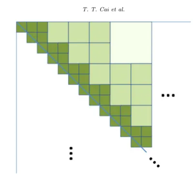
Now we briefly introduce the construction of blocks. First, we construct dis-joint square blocks of size kad logpalong the diagonal. Second, a new layer of blocks of sizekadare created towards the top right corner along the diagonal next to the previous layer. In particular, this layer of blocks has either two or one block (of size kad) in an alternating fashion (see Figure1). After this step, we note that the odd rows of blocks has three blocks of size kad and even rows of blocks have two blocks of size kad. This creates space to double the size of the blocks in the next step. We then repeat the first and second steps building
Fig 1. Construction of blocks with increasing dimensions away from the diagonal.
on the previous layer of blocks but double the size of the blocks until the whole upper half of the matrix is covered. In the end, the same blocking construction is done for the lower half of the matrix. It is possible that the last row and last column of the blocks are rectangular instead of being square. For the sake of brevity, we omit the discussion on these blocks. See Cai and Yuan (2012) for further details. By the construction, the blocks form a partition of {1, . . . , p}2. We list the indices of those blocks byB={B1, . . . , BN}, assuming there areN blocks in total. The construction of the blocks is illustrated in Figure1.
Once the blocks B are constructed, we define the final adaptive estima-tor ˆΣAda
CY by the following thresholding procedure on the blocks of the sam-ple covariance matrix ˆΣn. First, we keep the diagonal blocks of size kad con-structed at the very beginning, i.e., ( ˆΣAda
CY )B = ( ˆΣn)B for those B in the diagonal. Second, we set all the large blocks to 0, i.e., ( ˆΣAdaCY )B = 0 for all
B ∈ B with size(B) > n/logn, where for B = I ×J, size(B) is defined to be max{|I|,|J|}. In the end, we threshold the intermediate blocks adap-tively according to their spectral norm as follows. Suppose B = I×J. Then ( ˆΣAda
CY )B= ( ˆΣn)BI{||( ˆΣn)B||> λB}, where
λB = 6(||( ˆΣn)I×I|| · ||( ˆΣn)J×J||(size(B) + logp)/n)1/2. Finally we obtain the adaptive estimator ˆΣAda
CY , which is rate optimal over the classesFα(M0, M) orGα(M1).
Theorem 8(Cai and Yuan (2012)). Suppose thatXis sub-Gaussian distributed with some finite constant. Then for all α > 0, the adaptive estimator ΣˆAda CY
constructed above satisfies sup Fα(M0,M) EΣˆAda CY −Σ 2 ≤minC logp n +n − 2α 2α+1 ,p n ,
where the constant C depends onα,M0 andM.
In light of the optimal rate of convergence given in Theorem 1, this shows that the block thresholding estimator adaptively achieves the optimal rate over
Fα(M0, M) for all α >0. Estimation under other losses
In addition to estimating bandable covariance matrices under the spectral norm, estimation under other losses has also been considered in literature. Furrer and Bengtsson (2007) introduced a general tapering estimator, which gradually shrinks the off-diagonal entries toward zero with certain weights, to estimate covariance matrices under the Frobenius norm loss in different settings. Cai et al. (2010) studied the problem of optimal estimation under the Frobenius norm loss over the classesFα(M0, M) andGα(M1), and Cai and Zhou (2012a) investigated optimal estimation under the matrix 1 norm.
The optimal estimators for both the Frobenius norm and matrix1norm are again based on the tapering estimator (or banding estimator) with the band-widthkT ,F =n 1 2(α+1) andk T ,1= min n2(α1+1),(n/logp) 1 2α+1 respectively. The rate of convergence under the Frobenius norm of Fα(M0, M) is different from that of Gα(M1). The optimal rate of convergence under the matrix 1 norm is min
(logp/n)2α2α+1 +n−αα+1
, p2/n. Their corresponding minimax lower bounds are established in Cai et al. (2010) and Cai and Zhou (2012a). Com-paring these estimation results, it should be noted that although the optimal estimators under different norms are all based on tapering or banding, the best bandwidth critically depends on the norm under which the estimation accuracy is measured.
2.2. Toeplitz covariance matrices
We turn to optimal estimation of Toeplitz covariance matrices. Recall that ifX
is a stationary process with autocovariance sequence (σm), then the covariance matrix Σp×p has the Toeplitz structure such thatσij =σ|i−j|.
Wu and Pourahmadi (2009) introduced and studied a banding estimator based on the sample autocovariance matrix, and McMurry and Politis (2010) extended their results to tapering estimators. Xiao and Wu (2012) further im-proved these two results and established sharp banding estimator under the spectral norm. All these results are obtained in the framework of causal rep-resentation and physical dependence measures proposed in Wu (2005). One important assumption is that there is only one realization available, i.e.n= 1.
More recently, Cai, Ren, and Zhou (2013) considered the problem of optimal estimation of Toeplitz covariance matrices over the classFTα(M0, M). The re-sult is valid not only for fixed sample size but also for the general case when
n, p→ ∞.
An optimal tapering estimator is constructed by tapering the sample autoco-variance sequence. More specifically, recall ˆΣn = (ˆσij) is the sample covariance matrix. For 0≤m≤p−1, set
˜ σm= (p−m)−1 s−t=m ˆ σst,
which is an unbiased estimator of σm. The estimator ˜σmwas also proposed in Bickel and Levina (2004). Then the tapering Toeplitz estimator ˆΣT oepT ,k = (˘σst) of Σ with bandwidth k is defined as ˘σst = ω|s−t|σ˜|s−t|, where the weight
ωm is defined in (11). By picking the best choice of the bandwidth kT o = (np/log (np))2α1+1, the optimal rate of convergence is given as follows.
Theorem 9 (Cai, Ren, and Zhou (2013)). Suppose that X is Gaussian dis-tributed with a Toeplitz covariance matrix Σ ∈ FTα(M0, M) and suppose (np/log (np))2α1+1 ≤ p/2. Then the tapering estimator ΣˆT oep
T ,k with kT o = (np/log (np))2α1+1 satisfies sup Σ∈FTα(M0,M) EΣˆT oep T ,kT o−Σ 2≤C log(np) np 2α 2α+1 .
The performance of the banding estimator was also considered in Cai, Ren, and Zhou (2013). Surprisingly, the best banding estimator is inferior to the optimal tapering estimator over the classFTα(M0, M), which is due to a larger bias term caused by the banding estimator. See Cai, Ren, and Zhou (2013) for further details. At a high level, the upper bound proof is based on the fact that the spectral norm of a Toeplitz matrix can be bounded above by the sup-norm of the corresponding spectral density function. which leads to the appearance of the logarithmic term in the upper bound. A lower bound argument will be introduced in Section4.5. The appearance of the logarithmic term indicates the significant difference in the technical analyses between estimating bandable and Toeplitz covariance matrices.
2.3. Sparse covariance matrices
We now consider optimal estimation of another important class of structured covariance matrices – sparse covariance matrices. This problem has been con-sidered by Bickel and Levina (2008b), Rothman et al. (2009) and Cai and Zhou (2012a,b). These works assume that the variances are uniformly bounded, i.e., maxi σii ≤ ρ for some constant ρ > 0. Under such a condition, a uni-versal thresholding estimator ˆΣU,T h = σˆU,T h
ij
ˆ
σij ·I{|σˆij| ≥ γ(logp/n)1/2} for some sufficiently large constant γ = γ(ρ). This estimator is not adaptive as it depends on the unknown parameter ρ. The rates of convergencesn,p(logp/n)(1−q)/2under the spectral norm and matrix1 norm in probability are obtained over the classes of sparse covariance matrices, in which each row/column is in an q ball or a weak q ball, 0 ≤ q < 1. i.e. maxi
p
j=1|σij|q≤sn,p or max1≤j≤pσj[k] q
≤sn,p/krespectively. Sparse covariance matrices: Adaptive minimax upper bound
Estimation of a sparse covariance matrix is intrinsically a heteroscedastic prob-lem in the sense that the variances of the entries of the sample covariance matrix ˆ
σij can vary over a wide range. A universal thresholding estimator essentially treats the problem as a homoscedastic problem and does not perform well in general. Cai and Liu (2011a) proposed a data-driven estimator ˆΣAd,T h which adaptively thresholds the entries according to their individual variabilities,
ˆ ΣAd,T h= (ˆσijAd,T h), ˆθij = 1 n n k=1 (XkiXkj−ˆσij)2 (13) ˆ σijAd,T h= ˆσij·I{|σˆij| ≥δ(ˆθijlogp/n)1/2}.
The advantages of this adaptive procedure are that it is fully data-driven and no longer requires the variances σii to be uniformly bounded. The estimator
ˆ
ΣAd,T h attains the following rate of convergence adaptively over sparse covari-ance classesH(cn,p) defined in (4) under the matrixωnorms for allω∈[1,∞].
Theorem 10 (Sparse Covariance Matrices). Suppose each standardized com-ponent Yi=Xi/σ1ii/2 is sub-Gaussian distributed with some finite constant and a mild condition minijVar(YiYj)≥c0 for some positive constantc0. Then the adaptive estimatorΣˆAd,T h constructed above in (13) satisfies
inf H(cn,p) PΣˆAd,T h−Σ ω≤Ccn,p((logp)/n) 1/2≥1−O((logp)−1/2p−δ+2), (14) where ω∈[1,∞].
A similar idea was applied in the practical implementation without theoreti-cal justification in El Karoui (2008). The proof of Theorem10essentially follows
from the analysis in Cai and Liu (2011a) for ΣˆAd,T h under the
matrix 1 norm over a smaller class of sparse covariance matrices Uq∗(sn,p), where each row/column (σij)1≤i≤p is assumed to be in a weighted q ball, maxi(σiiσjj)(1−q)/2|σij|q ≤sn,p. That result is automatically valid for all ma-trixω norms, following the claim in Section 6 of Cai and Zhou (2012b), where the Riesz-Thorin interpolation theorem is applied. The key technical tool in the analysis is the following large deviation result for self-normalized entries of the sample covariance matrix.
Lemma 2. Under the assumptions of Theorem10, for any smallε >0,
P(|σˆij−σij|/θˆij1/2≥
Lemma 2 follows from a moderate deviation result in Shao (1999). See Cai and Liu (2011a) for further details.
Theorem 10states the rate of convergence in probability. The same rate of convergence holds in expectation with a mild sample size conditionp≥nφ for someφ >0. A minimax lower bound argument under the spectral norm is pro-vided in Cai and Zhou (2012b) (see also Section4.4), which shows that ˆΣAd,T h is indeed rate optimal under all matrix ω norms. In contrast, the universal thresholding estimator ˆΣU,T his sub-optimal overH(c
n,p) due to the possibility of maxi(σii)→ ∞.
Besides the matrix ω norms, Cai and Zhou (2012b) considered a unified result on estimating sparse covariance matrices under a class of Bregman diver-gence losses which include the commonly used Frobenius norm as a special case. Following a similar proof there, it can be shown that the estimator ˆΣAd,T h also attains the optimal rate of convergence under the Bregman divergence losses over the large parameter classH(cn,p). In addition to the hard thresholding es-timator introduced above, Rothman et al. (2009) considered a class of threshold-ing rules with more general thresholdthreshold-ing functions includthreshold-ing soft thresholdthreshold-ing, SCAD and adaptive Lasso. It is straightforward to extend all results above to this setting. Therefore, the choice of the thresholding function is not important as far as the rate optimality is concerned.
It is worthwhile to point out that all related results hold under assumptions on the marginals ofXonly. This is significantly different from other covariance ma-trices estimation problems, where joint distributional assumptions are typically imposed. Among these results, distributions with polynomial-type tails have been considered by Bickel and Levina (2008b), El Karoui (2008) and Cai and Liu (2011a). In particular, Cai and Liu (2011a) showed that the adaptive thresh-olding estimator ˆΣAd,T h attains the same rate of convergencec
n,p((logp)/n)1/2 as the one for the sub-Gaussian case (14) in probability over the classUq∗(sn,p), assuming that for some γ, C > 0, p ≤ Cnγ and for some > 0, such that E|Xj|4γ+4+≤Kfor allj. The superiority of the adaptive thresholding estima-tor ˆΣAd,T h for heavy-tailed distributions is also due to the moderate deviation for the self-normalized statistic ˆσij/θˆij (see Shao (1999)). It is easy to see that this still holds over the class H(cn,p). Recently, Chen et al. (2013) and Basu and Michailidis (2015) considered sparse covariance matrix estimation for time series data based on certain dependence measures, which play an important role in the rates of convergence. In particular, the results in Basu and Michailidis (2015) rely on a new measure of stability for stationary processes without using the commonly imposed functional dependence measure in Wu (2005).
Support recovery
A closely related problem to estimating a sparse covariance matrix is the recov-ery of the support of the covariance matrix. This problem has been considered by, for example, Rothman et al. (2009) and Cai and Liu (2011a). For support recovery, it is natural to consider the parameter space H0(cn,p). Define the
support of Σ = (σij) by supp (Σ) = {(i, j) :σij = 0}. Rothman et al. (2009) applied the universal thresholding estimator ˆΣU,T h to estimate the support of true sparse covariance inH0(cn,p), assuming bounded variances maxi(σii)≤ρ. In particular, it successfully recovers the support of Σ in probability, provided that the magnitudes of the nonzero entries are above a certain threshold, i.e., min(i,j)∈supp(Σ)|σij|> γ0(logp/n)1/2 for a sufficiently largeγ0>0.
Cai and Liu (2011a) extended this result under a weaker assumption on entries in the support using the adaptive thresholding estimator ˆΣAd,T h. We state the result below.
Theorem 11 (Cai and Liu (2011a)). Let δ ≥2. Suppose the assumptions in Theorem10 hold and for all(i, j)∈supp (Σ)
|σij|>(2 +δ+γ) (θijlogp/n)1/2,
for some constant γ >0, whereθij = Var (XiXj). Then we have inf
H0(cn,p)
P(supp( ˆΣAd,T h) = supp(Σ))→1.
2.4. Spiked sparse covariance matrices
Minimax upper bound
We now turn to the optimal estimation of sparse spiked covariance matrices over
J(cn,p, rn,p, λn,p) in (7) under the squared spectral norm loss. Recall the spiked covariance structure Σ =VΛV+Iis defined in (6). This structure was originally considered in Johnstone (2001) and have been studied by several papers under the sparse principal component analysis setting, including Paul (2007), Nadler (2008), Johnstone and Lu (2009), Amini and Wainwright (2009), Birnbaum et al. (2013), Ma (2013), Vu and Lei (2013), Cai et al. (2013), Berthet and Rigollet (2013) and Cai et al. (2015). However, most of the works considered estimating either individual leading eigenvector vi or the principal subspaceV V spanned by rn,p leading eigenvectors under the Frobenius norm loss. A brief discussion along this line is presented later in this section. Despite its close relationship with estimation of the covariance matrix Σ via the well-known sin-theta theorem (Davis and Kahan (1970)), the optimality estimation of sparse spiked covariance matrices cannot be obtained immediately, especially under the setting wherern,p andλn,p go to infinity asn, p→ ∞.
In a recent work, Cai et al. (2015) considered minimax estimation of sparse spiked covariance matrices under the squared spectral norm. The key step of constructing optimal estimators is a global searching scheme to find the support of V. More specifically, let the support of V be supp (V) = {i:Vi,∗=0} ⊂ {1, . . . , p}and the cardinality of any setSbeDS. Recall ˆΣ = (ˆσij) is the sample covariance matrix. Then the estimator of supp (V) is defined by an arbitrary
element in the following set
SV(cn,p) =
S⊂ {1, . . . , p}:DS =cn,p, and for allA⊂Sc withDA≤cn,p,
ΣˆA,A−I≤η(DA, n, p, γ),ΣˆA,S≤2ΣˆS,Sη(cn,p, n, p, γ)
,
where the thresholding quantity
η(a, n, p, γ) = 2 a n+ γ nalog(ep/a) + a n+ γ nalog(ep/a) 2 ,
with γ ≥ 10 under the Gaussian assumption. Intuitively, the two deviation criterions inSV(cn,p) admit supp (V) as a feasible element and at the same time rule out the possibility that Sc overlaps with supp (V) for anyS ∈ SV(c
n,p). The quantity η(a, n, p, γ) is carefully picked under the Gaussian assumption based on the Davidson-Szarek bound (Davidson and Szarek (2001)). See Cai et al. (2015) (also Proposition D.1 in Ma (2013)) for further details. Given an estimator ˆS ∈ SV(cn,p) of supp (V), the final sparse spiked covariance matrix estimator can be defined as
ˆ
ΣCM W =ˆσijCM W, where ˆσijCM W = ˆσijI{i∈S, jˆ ∈Sˆ}+ 1I{i=j /∈Sˆ}. (15) We set ˆΣCM W =I ifSV(cn,p) is the empty set. It was shown that the global search estimator ˆΣCM W attains the following rate of convergence under the spectral norm.
Theorem 12 (Cai et al. (2015)). Suppose that X is Gaussian distributed. If cn,p
n log
ep
cn,p ≤cfor a sufficiently small constant c >0, then
sup J(cn,p,rn,p,λn,p) EΣˆCM W −Σ2≤C (λn,p+ 1)cn,p n log ep cn,p +λ 2 n,prn,p n .
At a high level, the first term in the upper bound above does not involvern,p and is due to estimation of the leading eigenvector. The second term essentially follows from the estimation error of eigenvalue for acn,pbycn,pmatrix with rank
rn,p. It is clear that under the setting in which λn,p is bounded by a universal constant, the rate of convergence reduces to cn,p
n log
ep
cn,p since rn,p cannot be
larger than cn,p. Under such a setting, it is interesting to compare the rates of convergence overJ(cn,p, rn,p, λn,p) and a larger class H0(cn,p) considered in Section 2.3. Theorems 10and 12 imply that the rate is reduced from c
2 n,plogp n to cn,p n log ep
cn,p. This much faster rate of convergence can be achieved because
of the extra spike structure.
Unlike other estimators considered in the previous sections which are ob-tained from the sample covariance via a direct “smoothing” step, the estimator
ˆ
ΣCM W is obtained by a global search for the support of V, which is compu-tationally intensive. It is of interest to ask whether a compucompu-tationally efficient while still minimax optimal estimator exists. Consider a special case of rank one