Statistics Preprints Statistics
3-2009
Strategy for Planning Accelerated Life Tests with
Small Sample Sizes
Haiming Ma
Iowa State University, [email protected]
William Q. Meeker
Iowa State University, [email protected]
Follow this and additional works at:http://lib.dr.iastate.edu/stat_las_preprints
Part of theStatistics and Probability Commons
This Article is brought to you for free and open access by the Statistics at Iowa State University Digital Repository. It has been accepted for inclusion in Statistics Preprints by an authorized administrator of Iowa State University Digital Repository. For more information, please contact
Recommended Citation
Ma, Haiming and Meeker, William Q., "Strategy for Planning Accelerated Life Tests with Small Sample Sizes" (2009).Statistics Preprints. 61.
Strategy for Planning Accelerated Life Tests with Small Sample Sizes
AbstractPrevious work on planning accelerated life tests has been based on large-sample approximations to evaluate test plan properties. In this paper, we use more accurate simulation methods to investigate the properties of accelerated life tests with small sample sizes where large-sample approximations might not be expected to be adequate. These properties include the simulated s-bias and variance for quantiles of the failure-time distribution at use conditions. We focus on using these methods to find practical compromise test plans that use three levels of stress. We also study the effects of not having any failures at test conditions and the effect of using incorrect planning values. We note that the large-sample approximate variance is far from adequate when the probability of zero failures at certain test conditions is not negligible. We suggest a strategy to develop useful test plans using a small number of test units while meeting constraints on the estimation precision and on the probability that there will be zero failures at one or more of the test stress levels. Keywords
accelerated life testing, large-sample approximate variance, maximum likelihood, stress testing Disciplines
Statistics and Probability Comments
This preprint was published as Haiming Ma and W.Q. Meeker, " Strategy for Planning Accelerated Life Tests with Small Sample Sizes",IEEE Transactions on Reliability(2010): 610-619, doi:10.1109/TR.2010.2083251.
1
Strategy for Planning Accelerated Life Tests with Small Sample Sizes
Haiming Ma and W. Q. Meeker Department of Statistics
Iowa State University Ames, IA 50011
Abstract
Previous work on planning accelerated life tests has been based on large-sample approximations to evaluate test plan properties. In this paper, we use more accurate simulation methods to investigate the properties of accelerated life tests with small sample sizes where large-sample approximations might not be expected to be adequate. These properties include the simulated s-bias and variance for quantiles of the failure-time distribution at use conditions. We focus on using these methods to find practical compromise test plans that use three levels of stress. We also study the effects of not having any failures at test conditions and the effect of using incorrect planning values. We note that the large-sample approximate variance is far from adequate when the probability of zero failures at certain test conditions is not negligible. We suggest a strategy to develop useful test plans using a small number of test units while meeting constraints on the estimation precision and on the probability that there will be zero failures at one or more of the test stress levels.
Key Words – Large-Sample Approximate Variance, Maximum likelihood, Reliability,
2
Acronyms
ALT accelerated life test
ZFP1 problem when zero failures occur at one or more levels of stress
ZFP2 problem when zero failures occur at two or more levels of stress
ML maximum likelihood
CPPV critical point planning values
Notation
n total number of test units
U
s , sH pre-specified use level and highest level of stress
, L
s sM lowest and middle levels of stress
, L
π πM, πH allocations of test units at sL, sM and sH, respectively
ξ standardized stress level ξ =
(
s−sU) (
/ sH −sU)
t, η failure time and censoring time
σ
µ , location and scale parameters of a location-scale distribution
1 0 ,γ
γ parameters of the log-linear regression model
( )
⋅φ , Φ
( )
⋅ standard pdf and cdf, respectively, of a location-scale distributionH M L
U p p p
p , , , probabilities that a unit will fail by timeη at use, lowest, middle and
highest stress levels, respectively E
L
π , ( E
L
ξ ) allocation (lowest level of stress), corresponding to having an equal
expected number of failures at each of the three levels of stress for a fixed
3 Opt
L
π , ( Opt
L
ξ ) allocation and lowest level of stress, respectively, corresponding to overall
optimum (minimum) variance of the quantile estimators obtained by
adjusting πL and ξL, simultaneously.
p
z p quantile of a standard location-scale distribution
( )
ξp p y
y = p quantile of a location-scale distribution at stress level ξ
1
Introduction
1.1
Previous work
In an accelerated life test (ALT), units are tested at higher than usual levels of stress (e.g., temperature, voltage, or pressure) to obtain information about reliability in a small amount of
time.ALTs are commonly used in product design and testing processes (see, for example,
Chapter 6 of Nelson [11] and Chapters 18-20 of Meeker and Escobar [9]). Previous ALT
planning methods have been based on large-sample approximations to assess test plan properties. The test plan properties (and corresponding approximations) depend on the model parameters. Thus one needs planning values for the parameters. As suggested in [5], the planning values can be given in terms of convenient quantities such as failure probabilities at the highest and use stress levels, respectively. As suggested in [12] and [13] information for planning values can be obtained from previous experience with similar products and materials or engineering judgment. Optimized two-stress-level test plans based upon such planning values that achieve the smallest large-sample approximate variance of the maximum likelihood (ML) estimators of interest (see, for example, ref. [9, 11 and 13]) have been studied extensively. To be robust to possible
misspecification of the planning values and the relationship between the life and the levels of accelerating stress, compromise test plans with three or more levels have also been proposed and applied in practice [3, 7, 9 and 12].
4
1.2
Motivation
In practice, ALTs are usually subject to the constraint that the available number of test units has to be small either because of high cost of the units or availability of prototype units. In these cases, test planners may need to know the smallest possible number of units that are needed and how to choose the levels of stress and the allocation for those units to achieve a specified precision in the ML estimators.
We show how to find practical, statistically efficient constant-stress ALT plans with three levels of stress. When the sample sizes are small, test plans generated from large-sample
approximations may not be adequate. In this paper, we use large-sample approximations for initial guidance but turn to simulation to do the needed evaluation of the properties of small-sample test plans that are needed to choose an actual plan. We illustrate the methods with an example. The results show that ALT test plans for small samples can be distinctly different from those suggested by large-sample approximations.
1.3
Overview
The remainder of this paper is organized as follows. Section 2 presents the model upon which our evaluations are based and introduces an ALT example that we use to illustrate how to evaluate the test-plan properties with small samples. Section 3 evaluates optimized compromise test plans with small samples. Section 4 studies test plans with the smallest zero failure
probability and considers the impact of using incorrect planning values. Section 5 investigates the effect that using a small sample size will have on the adequacy of normal-approximation s-confidence intervals. Section 6 gives some concluding remarks and describes related areas for future research.
5
2
Model and Ml Estimation
2.1
Setup
As described in [3] and [11], most ALT models require a transformation of stress (e.g.,
log of voltage). We use s to denote this transformed stress. All of the stress levels in the ALT
will be between the use stress sU and a pre-specified highest stress sH. For convenience, we use
the standardized stress ξ =
(
s−sU) (
/ sH −sU)
, where sU ≤s≤sH and 0≤ξ ≤1. Thus ξU =0and ξH =1. All the test units are divided into three groups allocated at ξH , ξL, and ξM,
respectively, where the middle level of stress is ξM =
(
ξL +ξH)
2. We assume, as is the case inmost applications, that the three groups are tested simultaneously until a common censoring time
η. With practical values of the planning values, if one does not use the kind of constraint
suggested here (and in previous work with compromise ALT test plans), optimization results in an ALT plan with only two levels of stress (the optimum proportion at the middle level would approach zero or the optimum location of the middle level would approach one of the other two levels).
Constant-stress three-level compromise test plans can have a variety of forms. For example, Meeker and Escobar (see, Chapter 20 of [8]) suggest a compromise test plan with a
fixed allocation proportion of 0.2 at ξM. In this paper, we modify this compromise test plan in
the following way. Instead of a fixed πM, the allocations πL and πM at ξL and ξM,
respectively, are chosen such that the expected numbers of failures at ξL and ξM are equal. This
modified compromise test plan is more appropriate for small sample sizes because it does a better job of controlling the probability of having zero failures at the lower stress levels. Under
this constraint we choose Opt
L
ξ and Opt
L
π to obtain the optimized compromise test plan that
minimizes the variance of the ML estimators of a specific function of the ALT model
6
and conditioning on being able to estimate the model parameters) variances of the ML estimators by simulation and compare them with large-sample approximate variances. Our goal is to find an
easy-to-apply method to choose a useful test plan defined by
(
πL,ξL,n)
that has good statisticalproperties and that can achieve the precision desired by a practitioner.
2.2
Model
Our assumed model corresponds to that used in most previous work in this area,
summarized in Chapter 6 of [11] and Chapter 20 of [9]. At any level of the standardized stress ξ,
the log failure time Y follows a location-scale distribution with constant σ and a cdf
(
Y ≤ y)
=Φ[
(
y−µ)
σ]
Pr . The location parameter depends on (possibly transformed) stress
through the linear relationship µ =γ0 +γ1ξ , where γ0 and γ1 are the regression model
parameters. In our example, Φ
( )
z =Φsev( )
z =1−exp[
−exp( )
z]
is the standardized smallestextreme value distribution corresponding to a Weibull failure time distribution. The failure
probabilities at the highest stress and the use stress are pH = Φ[ log( )
(
η −γ0−γ1)
/ ]σ and(
)
[
log(η)−γ0 σ]
Φ=
U
p , respectively. It is easy to express the probability at any other stress
level ξ as a function of pU and pH. Given pH, pU, σ and η, one can easily calculate γ0 and
1
γ .
2.3
ML Estimation
Let γˆ0, γˆ1 and σˆ denote the ML estimators of γ0, γ1, and σ , respectively. Then the
ML estimator of the p quantile at stress level ξ can be expressed as yˆp =γˆ0 +γˆ1ξ +zpσˆ, where
p
z =Φ−1
( )
p . The large-sample approximate variance of yˆp is( ) (
yˆp 1, ,zp)
(
1, ,zp)
var
A = ξ Σγˆ0,γˆ1,σˆ ξ , where Σγˆ0,γˆ1,σˆ is the large-sample approximate
7 T
indicates vector transpose (for details on how to do the computations, see, for example, Chapter 20 of Meeker and Escobar [9]). As is common practice in the ALT planning literature, one can compare the relative efficiency of test plans with different samples sizes using the scaled
large-sample approximate variance denoted by
(
n σ2)
Avar( )
yˆp. For small sample sizes,
however, the scaled variance of yˆp denoted by
(
n σ2)
Var( )
yˆpcan be obtained to a much higher degree of approximation by using the Monte Carlos simulation, as described in detail in Section 2.4.
2.4
Zero failure problems
In ALTs with a fixed censoring time and small sample sizes, it is possible to have zero failures at one or more levels of stress at the end of the test. An ALT having zero failures at one or more levels of stress would generally be considered to be an unsuccessful ALT. Having zero failure at one or more levels of stress causes the loss of the advantages of a three-level test plan such as the ability to detect a departure from the assumed relationship between life and stress. We refer to this problem as the first type of zero failure problem (ZFP1). Having zero failures at two or more of the three levels of stress will make it impossible to estimate the model parameters or the quantile of interest. We refer to this problem as the second type of zero failure problem (ZFP2).
The s-bias and variance of yˆp can be obtained via simulations in the following way.
Based on the specified planning values, one can simulate sample ALT data. For each simulated
data set, one can calculate the ML estimators γˆ0, γˆ1, and σˆ and yˆp. Using a large number of
Monte-Carlo simulations, one can estimate E
( )
yˆp and Var( )
yˆp , conditional on no ZFP2(because when a ZFP2 problem arises in a simulation trial estimation of the model parameters is
8
ZFP2 [and thus, as we will see in our evaluations, such conditional variances could be misleading when Pr(ZFP2) is not negligible].
Generally, we want to find a test plan that has a small probability of having a ZFP1. Let L
n , nM and nH =n−nL −nM be the number of test units allocated at ξL, ξM and ξH,
respectively and let πi denote the allocation at stress level ξi where i = L, M and H. The number
of test units allocated to stress level i is ni =
[
πin]
, where n is the total sample size and[ ]
meansthe rounding to the nearest integer, because πin may not be an integer. The probability of failing
at ξi is 0 1 log( ) i i p η γ γ ξ σ − − = Φ . (1)
The relationship between πL and πM in our compromise test plan is πLpL =πMpM,
which implies an equal expected number of failures at ξL and ξM. Because all the test units are
s-independent, the probability of having zero failures at ξi can be expressed as
(
)
nii
i p
P = 1− , (2)
where i = L, M and H. Thus the probability of ZFP1 is
Pr(ZFP1) = PH + PM +PL −P PH L −P PM L −P PM H + P P PH M L. (3) Similarly, the probability of ZFP2 can be expressed as
Pr(ZFP2) = P PH L +P PM L +P PM H −P P PH M L (4) Given the levels of stress, the allocation corresponding to equal expected number of
failures at each of the three stress levels πiE can be calculated by the following formulas
L H H M M L M H E L p p p p p p p p + + = π (5) L H H M M L L H E M p p p p p p p p + + = π (6) L H H M M L L M E H p p p p p p p p + + = π . (7)
9
Given the three allocations, one can also calculate the lowest and middle levels of stress, E
L
ξ and E
M
ξ , to have an equal expected number of failures at each of the three levels of stress.
This can be done by noting that Pi, i = L, M and H depend on the ξi values and thus one can
solve the following equations for E
L ξ and E M ξ : M M H HP
π
Pπ
= (8) L L M MPπ
Pπ
= (9)Using (8) and the relationships (1) and (2), one can obtain E
M
ξ and E
L
ξ from (9).
From (3), one can obtain S
L
π , a value of πL to minimize Pr(ZFP1). However, we do not
have a simple analytical expression of S
L
π for given pL, pH and n. In practice, as is shown in
Section 3.3, S
L
π is close to and a little larger than E
L
π . Because E
i
π i = L, M and H do not depend
on the sample sizes, using E
i
π can make the following test plan specification and evaluation
simpler than using S
L
π .
2.5
The adhesive-bond ALT example and planning values
To illustrate the ideas presented in this paper, we will use the adhesive-bond test-planning example that was described in [7] and on page 535 of [9]. In this example, the
Weibull-distribution planning values were given as pH =0.9, pU =0.001, and σ =0.6, based on
previous experience with similar products. The censoring time is η = 183 days. The quantity of
interest is the 0.1 quantile (i.e., p = 0.1) of the failure-time distribution at the use stress level of
50 ºC. Using the above planning values, we obtain γ0 = 9.35, γ1 = −4.64and y0.1 = 8.0 by using
the formulas in Section 2.2. In the Meeker and Escobar [9] example, 300 units were available for testing. Here we will investigate test plans with fewer than 300 test units.
We will also assume there is uncertainty in the planning values. To do this we will
evaluate the compromise test plan properties using alternative planning values. In Section 4.2 we show that when considering misspecification of the three planning values for the parameters over the range of a cube, it is sufficient to do one further evaluation at one of the corners of the cube.
10
We call the planning values at this corner of the cube the critical point planning values or CPPV.
For our example the CPPV is pH = 0.45, pU = 0.0005 and σ = 0.75.
3
Evaluation of Optimized Compromise Test Plan with Small Samples
3.1
Zero failure problems of a previous compromise test plan
It is important to investigate the zero-failure behavior of the compromise test plans such
as those with a fixed πM proposed in [6] and [9]. Fixing πM = 0.2, one can obtain an optimized
(i.e., minimum Avar
(
yˆ0.1)
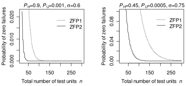
) compromise test plan by choosing πL = 0.531 and ξL = 0.638 underplanning values pH =0.9, pU =0.001, and σ =0.6. Figure 1 shows the probabilities of both
ZFP1 (dotted line) and ZFP2 (solid line) as a function of n when πL = 0.531 and ξL = 0.638 for
two points of planning values: pH =0.9, pU =0.001 and σ =0.6 (on the left) and pH = 0.45,
0005 . 0
=
U
p and σ =0.75 (on the right).
50 150 250 0 .0 0 0 0 .0 1 0 0 .0 2 0 PH=0.9, PU=0.001, σ=0.6
Total number of test units n
P ro b a b il it y o f z e ro f a il u re s ZFP1 ZFP2 50 150 250 0 .0 0 0 .0 4 0 .0 8 PH=0.45, PU=0.0005, σ=0.75
Total number of test units n
P ro b a b il it y o f z e ro f a il u re s ZFP1 ZFP2
Figure 1: Pr(ZFP1) (dotted line) and Pr(ZFP2) (solid line) as a function of n when
L
π = 0.531 and ξL = 0.638 for two sets of planning value( i) the original planning values: pH = 0.9, pU = 0.001 and σ = 0.6 (on the left) and (ii) the CPPV: pH = 0.45, pU = 0.0005 and σ = 0.75 (on the right).
11
Figure 1 shows that Pr(ZFP1) is much higher than Pr( ZFP2). This is because there are many more events leading to ZFP1 than ZFP2. Figure 1 also shows that the probabilities of having ZFP1 or ZPF2 under CPPV are much higher than the corresponding probabilities under the original planning values. Thus, it is important to consider the zero failure probabilities under both the original planning values and the corresponding CPPV.
To further investigate the cause of ZFP1 in Figure 1, consider PLM = PL +PM −PLPM ,
the probability of having zero failures at either ξL or ξM regardless of the number of failures at
H
ξ . If one plots PLM versus n on Figure 1, the curve would indistinguishable from the curve of
Pr(ZFP1) versus n in Figure 1. Thus ZFP1 is caused, primarily, by having no failures at either ξL
or ξM. To assure that there are failures at both ξL and ξM, practitioners should control Pr(ZFP1)
to be below some specified small value, say, 0.01.
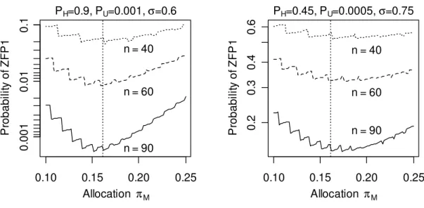
It is possible that an optimized compromise test plan with πM other than 0.2 may have a
smaller probability of ZFP1 than that for πM = 0.2. For each value of πM, there is a
corresponding optimized compromise test plan and a probability of ZFP1 associated with the
plan. Figure 2 shows Pr(ZFP1) of those optimized compromise test plans as a function of πM for
n = 40, 60 and 90 and the original planning values (on the left) and the CPPV (on the right). The
vertical dotted lines indicate the values of πM that result in having an equal expected number of
failures at ξL and ξM. The zigzag behavior comes from the integer sample-size rounding effect
12 PH=0.9, PU=0.001, σ=0.6 n = 40 n = 60 n = 90 Allocation πM P ro b a b il it y o f Z F P 1 0 .0 0 1 0 .0 1 0 .1 0.10 0.15 0.20 0.25 PH=0.45, PU=0.0005, σ=0.75 n = 40 n = 60 n = 90 Allocation πM P ro b a b il it y o f Z F P 1 0 .2 0 .3 0 .4 0 .6 0.10 0.15 0.20 0.25
Figure 2: Pr(ZFP1) of optimized compromise test plans as a function of πM for n = 40, 60 and 90 and two
sets of planning values: (i) the original planning values (pH = 0.9, pU = 0.001 and σ = 0.6) on the left and (ii) the CPPV (pH = 0.45, pU = 0.0005 and σ = 0.75) on the right. The vertical dotted lines show the value of πM at which the expected numbers of failures at ξL and ξM are equal.
Figure 2 shows that there is a value of πM at which Pr(ZFP1) is minimum for a specific
sample size. The value of πM is close to that of an optimized compromise test plan with an equal
expected number of failures at ξL and ξM [i.e., (9) holds]. Thus, to achieve, in a simple way, a
small ZFP1 probability when the sample sizes are small, we suggest using a compromise test
plan with an equal expected numbers of failures at ξL and ξM. In the remainder of this paper,
the term compromise test plans refers only to the compromise test plans with an equal expected
number of failure at ξL and ξM.
3.2
Adequacy of the large-sample approximate variance
Figure 3 shows the scaled actual variance
(
2)
(
0.1)
ˆ Var y
n σ conditional on no ZFP2 (on
the left) and the corresponding Pr(ZFP1) (on the right) as a function of the total sample size n,
under the different planning values and test plans. The horizontal lines on the left plots show
(
)
(
0.1)
2
ˆ Avar y
13
data generated from the compromise test plan with an equal expected failure number at ξL and
M
ξ described in Section 3.1. These figures provide an assessment of the adequacy of the large
sample approximation for
(
2)
(
0.1)
ˆ Var y
n σ and we can see when the approximation may be
inadequate when n is too small.
pH=0.9, pU=0.001, σ=0.6 1 0 0 1 4 0 1 8 0 2 2 0 2 6 0 20 50 100 200 500 1000 πL=0.537, ξL=0.773 πL=0.553, ξL=0.637
Total number of test units n
(n / σ 2 )V a r( y^0.1 ) pH=0.9, pU=0.001, σ=0.6 0 0 .0 5 0 .1 5 0 .2 5 20 50 100 200 500 1000 πL=0.537, ξL=0.773 πL=0.553, ξL=0.637 0.01
Total number of test units n
P ro b a b il it y o f Z F P 1 pH=0.45, pU=0.0005, σ=0.75 1 0 0 2 5 0 4 0 0 5 5 0 7 0 0 20 50 100 200 500 1000 πL=0.537, ξL=0.773 πL=0.526, ξL=0.649
Total number of test units n
(n / σ 2 )V a r( y^0.1 ) pH=0.45, pU=0.0005, σ=0.75 0 0 .0 5 0 .1 5 0 .2 5 20 50 100 200 500 1000 πL=0.537, ξL=0.773 πL=0.526, ξL=0.649 0.01
Total number of test units n
P ro b a b il it y o f Z F P 1
Figure 3: The plots on the left side are the smoothed scaled variances
(
2)
(
0.1)
ˆ Var yn σ , conditional on no ZFP2 as a function of n under original planning values (top) and the CPPV (bottom). The horizontal lines
show the corresponding
(
n σ2)
Avar(
yˆ0.1)
. The simulated curves are based on 10,000 simulations at each point using the Weibull distribution model under the compromise three–level constant-stress test plans with an equal expected number of failures at ξL and ξM. The plots on the right sideshow the corresponding Pr(ZFP1) calculated by using (3). The dotted horizontal lines indicate where Pr(ZFP1) = 0.01.14
Figure 3 shows for the original planning values (top) and the CPPV (bottom), the
optimized [i.e., the minimumAvar
(
yˆ0.1)
] compromise test plans obtained by adjusting πL andL
ξ . For the original planning values, the optimized compromise test plan has πL = 0.553 and ξL
= 0.637. For the CPPV planning values, the optimized compromise test plan has πL = 0.526 and
L
ξ = 0.649. As expected, given the same planning values and number of test units, compared
with the non-optimized test plans, the optimized test plans provide smaller variances at the expense of a higher probability of ZFP1.
Another important observation from Figure 3 is that
(
2)
(
0.1)
ˆ Var y
n σ , conditional on no
ZFP2, first increases with n until a maximum value and then decreases, approaching
(
)
(
0.1)
2 ˆ
Avar y
n σ for large n. The maximum value of
(
2)
(
0.1)
ˆ Var y
n σ can be as high as around
40% larger than
(
2)
(
ˆ0.1)
Avar y
n σ . The maximum value occurs when the probability of ZFP2 is
between 0.01 and 0.02. The reason for this phenomenon is that when ZFP2 < 0.01, the
probability of ZFP2 decreases rapidly with n, resulting in less conditioning and a more accurate
representation of the true (unconditional) sample variability.
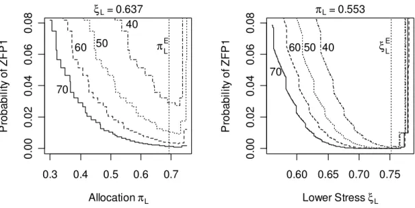
3.3 Reduction of the risk of ZFP1
Figure 4 shows Pr(ZFP1) as a function of the allocation πL (left) or ξL (right) when ξL
= 0.637 or πL = 0.553, respectively. These probabilities were computed from the original
planning values. Again, the zigzag behavior comes from the integer sample-size rounding effect described in Section 2.4.
15 0.3 0.4 0.5 0.6 0.7 0 .0 0 0 .0 2 0 .0 4 0 .0 6 0 .0 8 ξL = 0.637 Allocation πL P ro b a b il it y o f Z F P 1 70 60 50 40 πLE 0.60 0.65 0.70 0.75 0 .0 0 0 .0 2 0 .0 4 0 .0 6 0 .0 8 πL = 0.553 Lower Stress ξL P ro b a b il it y o f Z F P 1 70 60 50 40 ξLE
Figure 4: Pr(ZFP1) as a function of the unit allocation πL (left) and the lowest level of stress ξL (right) at L
ξ = 0.637 or πL = 0.553, respectively, for n = 40, 50, 60, and 70 with the original planning values
H p = 0.9, U
p = 0.001, and σ =0.6. The dotted vertical lines correspond to πLE = 0.692 and ξLE= 0.752, respectively.
In Figure 4, the left-hand plot shows that when πL increases from πL= 0.3, Pr(ZFP1)
(primarily occurring at ξL or ξM in this situation) decreases until πL ≈πLE. When πL increases
beyond πLE a value obtained from (5), Pr(ZFP1) (primarily occurring at ξH) will ultimately
increase. The right-hand plot in Figure 4 shows that when ξL increases beyond ξL = 0.56,
Pr(ZFP1) (primarily occurring at ξL or ξM in this situation) decreases until ξL ≈ξLE, [where ξLE
is obtained by solving (8) and (9)]. When ξL increases beyond ξLE, Pr(ZFP1) (primarily
occurring at ξH) will, again, ultimately increase. To have more precise estimation with small
sample sizes while controlling Pr(ZFP1) to be small, we suggest selecting πL or ξL to be
smaller than or close to πLE or ξLE, respectively.
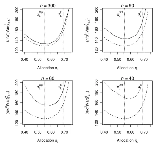
3.4
E
valuating the compromise test planIt is interesting to examine the relationship between the simulated actual variance and the large sample approximate variance under the compromise test plans for finite sample sizes. We
16
( Opt
L
π = 0.553, Opt
L
ξ = 0.637), corresponding to the large-sample approximate optimized
compromise test plan for the original planning values pH =0.9, pU =0.001, and σ = 0.6.
Figure 5 shows
(
2)
(
0.1)
ˆ Var y
n σ (solid and dotted curves) conditional on no ZFP2 and
(
)
(
0.1)
2 ˆ
Avar y
n σ (dashed curves), both as a function of the allocation πL with four different
values of n and a fixed ξL. The parts of the curves with dotted lines in Figure 5 represent the
values of πL where Pr(ZFP1) ≥ 0.01. The
(
2)
(
ˆ0.1)
Avar y
n σ curves are, of course, the same for
all sample sizes. The two vertical dotted lines represent Opt
L
π (on the left) and E
L
π (on the right).
These allocations can be calculated directly from (5), (8), and (9).
` 0.40 0.50 0.60 0.70 1 2 0 1 4 0 1 6 0 1 8 0 2 0 0 n = 300 Allocation πL ( n / σ 2 )V a r( y^0.1 ) πLE πLOpt 0.40 0.50 0.60 0.70 1 2 0 1 4 0 1 6 0 1 8 0 2 0 0 n = 90 Allocation πL ( n / σ 2 )V a r( y^0.1 ) πLE πLOpt 0.40 0.50 0.60 0.70 1 2 0 1 4 0 1 6 0 1 8 0 2 0 0 n = 60 Allocation πL ( n / σ 2 )V a r( y^0.1 ) πLE πLOpt 0.40 0.50 0.60 0.70 1 2 0 1 4 0 1 6 0 1 8 0 2 0 0 n = 40 Allocation πL ( n / σ 2 )V a r( y^0.1 ) πLE πLOpt Figure 5: Smoothed
(
2)
( ) 0.1 ˆ Varnσ y conditional on no ZFP2 and
(
n σ2)
Avar(
yˆ0.1)
for the Weibull distribution failure-time model as a function of the allocation πL based on 10,000 simulations at each point17
with ξL = 0.637 and the original planning values. The dashed lines show
(
2)
(
0.1)
ˆ Avar y
nσ . The two vertical dotted lines represent πLOpt and πLE, respectively. The dotted parts of the smoothed curves correspond to the values of πL where Pr(ZFP1) ≥ 0.01.
The simulated
(
2)
(
)
0.1
ˆ Var
n σ y is larger than the large-sample approximate
(
)
(
0.1)
2 ˆ
Avar y
n σ . When n = 300, 90, and 60 the minimum
(
2)
(
)
0.1
ˆ Var
n σ y occurs at a value
of πL close to πOptL [based on minimizing
(
n σ2)
Avar(
yˆ0.1)
] . For n = 40 the minimum scaledvariance is importantly larger than πLOpt. These results suggest that even when Avar
( )
yˆp doesnot provide a good approximation for Var
( )
yˆp , it can provide a good approximation forminimizing
(
2)
(
)
0.1
ˆ Var
n σ y as long as Pr(ZFP1) is not too large.
Another observation from Figure 5 is that, in the vicinity of πLE,
(
2)
(
)
0.1
ˆ Var
n σ y is
smaller when πL < πLE than when πL > πLE. When πL < πLE, Pr(ZFP1) due to no failures at
L
ξ or ξM is higher than that at ξH. When πL > πLE, Pr(ZFP1) due to no failures at ξH is higher
than that at ξL or ξM. Because there is a distinct increase in
(
2)
(
)
0.1
ˆ Var
n σ y at πLE when
compared to that at πOptL , as long as a specific criterion for the risk of ZFP1, say, Pr(ZFP1) ≤
0.01, is satisfied, one should select a πL < πLE to reduce
(
2)
(
)
0.1
ˆ Var
n σ y .
Figure 6 is similar to Figure 5, showing
(
2)
(
)
0.1
ˆ Var
n σ y and
(
n σ2)
Avar(
yˆ0.1)
as afunction of ξL with four different values of n and a fixed value of πL. Again, the dotted parts of
the curves show where Pr(ZFP1) ≥ 0.01. The two vertical dotted lines indicate the location of
Opt L
18 0.4 0.5 0.6 0.7 0.8 1 2 0 1 4 0 1 6 0 1 8 0 2 0 0 n = 300 Lower Stress ξL ( n / σ 2 )V a r( y^0.1 ) ξLOpt ξLE 0.4 0.5 0.6 0.7 0.8 1 2 0 1 4 0 1 6 0 1 8 0 2 0 0 n = 90 Lower Stress ξL ( n / σ 2 )V a r( y^0.1 ) ξLOpt ξLE 0.4 0.5 0.6 0.7 0.8 1 2 0 1 4 0 1 6 0 1 8 0 2 0 0 n = 60 Lower Stress ξL ( n / σ 2 )V a r( y^0.1 ) ξLOpt ξ L E 0.4 0.5 0.6 0.7 0.8 1 2 0 1 4 0 1 6 0 1 8 0 2 0 0 n = 40 Lower Stress ξL ( n / σ 2 )V a r( y^0.1 ) ξLOpt ξ L E Figure 6: Smoothed
(
2)
(
)
0.1 ˆ Varn σ y conditional on no ZFP2 for the 0.1 quantile (solid or dotted curves) of the Weibull failure distribution as a function of the lowest level of stress ξL from 10,000 simulations in each point with πL = 0.553 and the planning valuespH = 0.9, pU = 0.001 and σ = 0.6. The dashed lines represent
(
2)
(
0.1)
ˆ Avar y
n σ . The two vertical dashed lines represent ξLOpt (the left) and ξLE (the right). The dotted parts of the curves correspond to values of ξL where Pr(ZFP1) is larger than 0.01.
When n = 300, the minimum
(
2)
(
)
0.1 ˆ Var
n σ y occurs very close to ξLOpt, the optimized
lowest level of stress under the large-sample approximation. Note, however, that
(
2)
(
)
0.1 ˆ Var
n σ y
is always larger than
(
2)
(
0.1)
ˆ Avar y
n σ for n = 300. When n = 90, the simulated scaled variance
(the dotted line) is increasing in ξL when ξL < 0.45. When ξL > 0.5,
(
2)
(
)
0.1 ˆ Var
n σ y decreases
in ξL until it reaches a minimum, after which it increases. When n = 60 or 40, the conditional
(
2)
(
)
0.1 ˆ Var
19
after a turning point. At the turning point the probability of ZFP2 is between 0.01 and 0.02,
similar to the phenomenon described in Section 3.2. When ξL becomes larger, after passing
through a minimum point,
(
2)
(
)
0.1 ˆ Var
n σ y is increasing in ξL again. The values of ξL at the
minimum point are a little larger than Opt
L
ξ . Note that the small values of the conditional
(
2)
(
)
0.1 ˆ Var
nσ y are of little use when the probability of ZFP2 is importantly large (say greater
than 0.01).
Another observation from Figure 6 is that, in the vicinity of E
L ξ ,
(
2)
(
)
0.1 ˆ Var n σ y is smaller when ξL < E L ξ than when ξL > E L ξ . When ξL < E L ξ , Pr(ZFP1) is higher at ξL and ξM. When ξL > E Lξ , Pr(ZFP1) is higher at ξH. Because there is an important increase of the variance
at E
L
ξ when compared to that at Opt
L
ξ , as long as a specific criterion to the risk of ZFP1 say,
Pr(ZFP1) ≤ 0.01, is satisfied, one should select a ξL < E
L
ξ to reduce the variance.
Figures 5 and 6 show that, when Pr(ZFP1) ≤ 0.01, although
(
2)
(
)
0.1 ˆ Var n σ y ≥
(
)
(
0.1)
2 ˆ Avar yn σ , their minimum points in term of
(
πL, ξL)
for different values of n are close toeach other. This implies that the easy-to-compute
(
)
(
0.1)
2 ˆ
Avar y
n σ can be used as a guide to find
an initial test plan.
Based on the information given in Section 3, we use the following strategy to find a useful ALT plan.
1. Use the simple analytical formulas in Section 2.4 to determine the region of
(
πL, ξL, n)
in which Pr(ZFP1) is below the practitioner’s ZFP1 critical level (say 0.01).
2. Minimize
(
n σ2)
Avar( )
yˆp , subject to the constraint that Pr(ZFP1) is less than the ZFP1critical level, to obtain a tentative test plan.
3. Run simulations in the region of the tentative plan to fine tune the choice of πL and ξL
20
4
Test Plan Selection
4.1 Test plan properties for given planning values
Figure 7 is a contour plot showing
(
)
(
0.1)
2 ˆ
Avar y
n σ and Pr(ZFP1) as a function of ξL and
L
π using the compromise three-level test plan described in Section 3.4. The contours show
(
)
(
0.1)
2 ˆ
Avar y
n σ and the zigzag parallel lines show Pr(ZFP1) for different sample sizes. Again,
the zigzag behavior comes from the integer sample-size rounding effect described in Section 2.4.
The solid line labeled E
L
π ~ E
L
ξ shows where there is an equal expected number of failures at ξL
and ξH. This line can be obtained by plotting πLE as a function of ξL, or equivalently by plotting
E L
ξ as a function of πL. The region below this line is where we will find a useful test plan.
0.60 0.65 0.70 0.75 0 .4 0 0 .5 0 0 .6 0 0 .7 0 Lower Stress ξL A ll o c a ti o n πL πLE~ξLE + 1.10VOpt 1.017VOpt n=60 n=50 n=60 n=50 Pr(ZFP1) = 0.01 Pr(ZFP1) = 0.002
Figure 7: Contour plot showing
(
2)
(
ˆ0.1)
Avar yn σ and ZFP1 for the Weibull distribution model and the original planning values. The symbol “+” at the point (πL = 0.553, ξL = 0.637) indicates the location of the minimum
(
2)
(
0.1)
ˆ Avar y
21
Pr(ZFP1) (the dashed: 0.01 and the dotted: 0.002) for n = 50 and 60, respectively. The solid line labeled E
L
π ~ E
L
ξ shows where the expected numbers of failures at ξL and ξH are equal.
Figure 7 illustrates the simple strategy to find a test plan. First, one can draw several zigzag lines representing a small ZFP1 probability, say 0.01, for different sample sizes. Then, draw the contours of the scaled large-sample approximate variance. Along a zigzag line (corresponding to a sample size and a ZPF1 constraint), a point that is close to a contour is a
suitable candidate for the desired test plan having the smallest Avar
( )
yˆp for a specified samplesize and small ZFP1 probability. Considering different zigzag lines, one can evaluate the tradeoff between sample size and Pr(ZFP1) to get the desired precision.
4.2 Test planning with uncertain of planning values
Because there is always some degree of misspecification in the planning values, it is important to check the impact that the uncertainty of planning values will have on the variance, the ZFP1 probability and the choice of test plan for small sample sizes. For the adhesive-bond
example, if the practitioner is confident that the true values of pH, pU, and σ are in the
intervals (0.45, 0.95), (0.0005, 0.0015), and (0.45, 0.75), respectively, based on previous experience, separate contour plots could be made for each combination and these could be used to find a plan that is satisfactory over the region of planning value uncertainty.
Suppose that the ranges of the planning-values uncertainty can be described by a cube
containing all possible true values of (pH, pU, σ ). There are eight corners in the cube. Note
that Avar
( )
yˆp increases as σ increases and as pH or pU decreases, and the ZFP1 probabilityincreases as pH or pU decreases. Therefore, the corner with the smallest pH and pU and the
largest σ represents the largest possible values of both variance and the ZFP1 probability
22
value point (CPPV), becauseonce the variance and Pr(ZFP1) at this set meet certain
requirements, these requirements will be satisfied automatically throughout the entire cube. Thus, it is sufficient to investigate this critical point to evaluate the maximum impact of the incorrect planning values.
Figure 8 illustrates our procedure to find a good starting ALT test plan.
0.65 0.70 0.75 0.80 0 .4 0 0 .5 0 0 .6 0 0 .7 0 Lower Stress ξL A ll o c a ti o n πL x + O n = 80 1.29VOpt O 1.17VOpt C 1.05VOpt C πLE~ξLE VOpt O = 128.7 VOpt C = 414.8
Figure 8: Contour plots illustrating the procedure to find a good starting ALT test plan (details in the text).
The contours in Figure 8 show
(
)
(
0.1)
2
ˆ Avar y
n σ , relative to the value at minimum, when
the true parameters are equal to the CPPV (solid lines) and the original planning values (dashed
line). The “x” point indicates the position of the minimum pointπL = 0.526 and ξL = 0.649
where
(
)
(
0.1)
2
ˆ Avar y
n σ = 414.8 when the true parameters are equal to the CPPV. The “+” point
23
original planning values. The solid curve labeled E
L
π ~ E
L
ξ shows where there is an equal
expected number of failures at ξL and ξH when the true parameters are equal to the CPPV. The
zigzag line is where Pr(ZFP1) = 0.01 for n = 80. The dashed contour represents
(
)
(
0.1)
2 ˆ
Avar y
n σ ,
relative to the minimum when the true parameters are equal to the original planning values. The
small circle indicates the point along the zigzag line where
(
)
(
0.1)
2 ˆ
Avar y
n σ is minimized and
thus gives the tentative candidate test plan (πL = 0.537, ξL = 0.773 and n = 80) when the true
parameters are equal to the CPPV, thus taking into consideration the impact of the incorrect
planning values. Note that Figure 3 shows
(
2)
(
)
0.1 ˆ Var
n σ y conditional on no ZFP2 as a function
of sample size when the test plans are chosen at the three points “x”, “+” and the small circle.
Suppose that we desire to have Pr(ZFP1) ≤ 0.01 and Var
(
yˆ0.1)
≤ 4.6 at the CPPV. At thesame time, the sample size should be as small as possible. Computing properties of the test plan
at the small circle shows that, under the CPPV, Avar
(
yˆ0.1)
= 3.76. From Figure 3, there isroughly a 20% increase from
(
n σ 2)
Avar(
yˆ0.1)
to(
)
(
0.1)
2 ˆ
Var y
n σ when n = 80 and Pr(ZFP1)
= 0.01 under the CPPV. Thus the actual Var
(
yˆ0.1)
under the CPPV will be approximately1.2 3.76× =4.5. Therefore, the test plan with πL = 0.537, ξL = 0.773 and n = 80 is a candidate
that meets our criteria at the CPPV. Using the same test plan with n = 80 and assuming that the
values of the true parameters pH, pU, and σ are equal to the original planning values, we
obtainVar
(
yˆ0.1)
≈1.0 using similar calculations.
4.3 Verification of the candidate test plan
Section 4.2 showed how to find a candidate test plan to control the Pr(ZFP1) and
minimize
(
n σ2)
Var(
yˆ0.1)
. Because there is uncertainty in the adequacy of the large sampleapproximate variance used in the initial optimization, however, the candidate test plan needs to be verified by more accurate simulations. To do this for the adhesive bond example, we examine the simulated scaled variance around the small circle along the zigzag line in Figure 8.
24
The solid lines in Figure 9 show the conditional
(
n σ2)
Var(
yˆ0.1)
as a function of πLwhen n = 80,corresponding to the point (πL, ξL) on the zigzag line shown in Figure 8. The
dashed zigzag curves show
(
n σ2)
Avar(
yˆ0.1)
. The plots on the left (right) are for the situationwhen the true parameters are equal to the original planning values (equal to the CPPV). The zigzag behavior of the curves is again the result of changing discrete allocations of test units to
the stress levels. The location of πL where the smallest
(
n σ2)
Var(
yˆ0.1)
occurs under theCPPV is consistent with what is implied by Figure 8. In particular, along the zigzag line in Figure 8, the test plan around the point “O” has the smallest variance under the CPPV. The
actual Var
(
yˆ0.1)
values are 0.93 and 4.57 under the original planning values and the CPPV,respectively. 0.40 0.45 0.50 0.55 2 0 0 2 2 0 2 4 0 pH=0.9, pU=0.001, σ=0.6 Allocation πL (n / σ 2 )V a r( y^0.1 ) 0.40 0.45 0.50 0.55 5 5 0 6 5 0 7 5 0 pH=0.45, pU=0.0005, σ=0.75 Allocation πL (n / σ 2 )V a r( y^0.1 ) Figure 9: Simulated
(
2)
(
0.1)
ˆ Var yn σ (smoothed solid lines) conditional on no ZFP2 and
(
n σ2)
Avar(yˆ0.1) (dashed lines) for the 0.1 quantile of the Weibull failure distribution as a function of πL from 10,000 simulations at each point, while the point (πL, ξL) is on the zigzag line shown in Figure 8 where Pr(ZFP1) = 0.01 with n = 80 under the CPPV. The left plot is for the original planning valuesH
p = 0.9, pU = 0.001 and σ = 0.6 and the right is for the CPPV pH = 0.45, pU = 0.0005 and σ = 0.75 .
25
Figures 8 and 9 illustrate the strategy to select a useful test plan that has a low risk of ZFP1 while achieving the smallest possible variance after considering the uncertainty of
planning values. Note that constructing Figure 8 does not need any simulation. Thus this strategy minimizes the number of simulations that are needed and can allow one to find a useful test plan quickly.
Recall that Figure 2 shows that Pr(ZFP1) for a test plan with an equal expected number of
failures at ξL and ξM is close to but may not be the minimum for a specific sample size due to
the zigzag nature of Pr(ZFP1). Thus, it might be possible to find a slightly better test plan
without the constraint of equal expected failure numbers at ξL and ξM around the small circle.
Finally, we would like to point out that the reason why we only consider the variance and not the s-bias of the quantile estimators is because, under the assumed model, the s-bias
contribution to mean square error is negligible compared with variance when we control the risk of ZFP1 to be small.
5
Possible departure from the normal approximation for s-confidence
intervals
Normal approximation s-confidence intervals are based on the assumption that the
quantity zˆp =
(
yˆp−yp)
Varˆ( )
yˆp can be approximated by the standard normal distribution,where Varˆ
( )
yˆp is usually the local-information estimator of Var( )
yˆp . We call zˆp a “t-like”statistic because of its similarity to the t-statistic used in normal-distribution inference.
Especially when doing accelerated life testing with a small number of test units, the normal-distribution approximation may be inadequate when the expected number of failures is small. Here we show how to study the possible departure of actual coverage from the normal
26
Figure 10 shows normal Q-Q plots of zˆ0.1 for n = 80, obtained from 1,000 simulations
from the optimized compromise test plan(πL = 0.553, ξL = 0.637) on the left, and the
recommended test plan (πL = 0.537, ξL = 0.773) on the right, for the true parameters pH = 0.9,
U
p = 0.001, σ = 0.6 (top), and the true parameters pH = 0.45, pU = 0.0005, σ = 0.75
(bottom), respectively. These two points in the parameter space correspond to the original planning values and the CPPV. Except for the plot on the NE of Figure 10, all of the plots show departures from the normal distribution in the upper tail. Interestingly, the departures are not too bad in the lower tail for the recommended plans on the NW and SE of Figure 10. Note, however,
that a deviation in upper (lower) tail of the t-like statistics will lead to a lower (upper)
s-confidence bound with poor coverage properties. In reliability applications, it is usually the lower bound on a quantile that is of most interest.
27
Figure 10: Normal Q-Q plots of zˆ0.1 the simulated standardized variance conditional on no ZFP2 of the 0.1 quantile of the Weibull failure time distribution for n = 80, obtained from 1,000 simulations at test plans (
L π = 0.553, ξL = 0.637) on the left and (πL = 0.537, ξL = 0.773) on the right for the true parameters to be the original planning values (top) and the CPPV (bottom), respectively.
Table 1 shows the expected number failing at each test condition for each combination of test plan and planning values. As suggested by Table 1, the normal approximation tends to be especially poor when the expected number of failures at the individual test conditions is small. These results suggest that when the expected number of failures is small, one should use better s-confidence interval procedures such as those based on the bootstrap (see for example [4]) or the
28
inversion of a likelihood ratio test (see for example [14]) to have a procedure with a more accurate coverage probabilities.
Table 1:Expected numbers of failures for different situations when the sample size is 80.
True Parameters Test Plan Figure 10
Expected Numbers of Failures L
ξ ξM ξH Total
Original planning values Optimized NW 5.7 5.7 20.2 31.6 Original planning values Recommended NE 14.1 14.1 12.7 40.9
CPPV Optimized SW 2.0 2.0 10.3 14.3
CPPV Recommended SE 4.8 4.8 7.4 17.0
6
Concluding Remarks and Areas for Future Research
In this paper, we address the issues involved in planning ALTs with small sample sizes. We describe and investigate the important role that the possibility of zero failures can have on the conditional variance. For constant 3-level ALT plans, using a compromise test plan with an equal expected number of failures at the lowest and middle levels of stress can reduce the ZFP1 probability so that smaller sample sizes become possible for a specified estimation precision and set of planning values. Furthermore, by using the plots of test plans such as those shown in Figure 8, one can select a tentative test plan without having to run time-consuming simulations. Then the tentative test plan needs to be fine-turned and verified by simulations. Finally, one needs to check whether the commonly-used normal approximation for s-confidence intervals provides an adequate approximation or not.
Due to the small sample sizes involved, there is not a simple theory to provide the actual variance over a large parameter range, as provided by the large sample approximations.
29
plan using simulations. Applying the ideas in this paper to other models and distributions should be straightforward.
In this paper we show how to construct a three-level compromise constant-stress test plan with small sample sizes. If using the smallest number of test units is a primary concern, one might want to use a simple two-level test plan. The planning methods for the three-level stress test plan with small sample sizes can also be used to find a two–level constant-stress test plan with a small sample size. Simulations (for example, [4] and [14]) have shown that the adequacy of large sample approximation is closely related to the expected number of failures. Finally, we point out that it may be more appropriate to replace the term “small samples“ used in this paper as “small expected numbers of failures,” because under certain planning values, the expected number of failures is often small even if large numbers of test units are used.
References
[1] L. A. Escobar and W. Q. Meeker, “Planning Accelerated Life Tests with Two or More
Experimental Factors,” Technometrics, vol. 37, pp. 411-422, 1995.
[2] L. A. Escobar and W. Q. Meeker, “The Large-Sample Approximate Equivalence of the
Fisher Information Matrices for Type I and Type II Censored Data from Location-Scale
Families,” Communication of Statistics-Theory: Theory and Methods, vol. 30, pp.
2211-2225, 2001.
[3] L. A. Escobar, and W. Q. Meeker, “A Review of Accelerated Test Models,” Statistical
Science, vol.21, pp. 552–577, 2006.
[4] S. L. Jeng, and W. Q. Meeker, “Comparison of Approximate Confidence Interval
Procedures for Type I Censored Data,” Technometrics, vol. 42, pp. 135-148, 2000.
[5] W. Q. Meeker, “A Comparison of Accelerated Life Test Plans for Weibull and
Lognormal Distributions and Type I Censoring,” Technometrics, vol. 26, pp. 157-172,
30
[6] W. Q. Meeker and W. Nelson, “Optimized Accelerated Life Tests for Weibull and
Extreme Value Distributions,” IEEE Transactions on Reliability, vol. 24, pp. 321-322,
1975.
[7] W. Q. Meeker, and G. J. Hahn, “How To Plan An Accelerated Life Test-Some Practical
Guidelines,” Volume 10 in the American Society for Quality Control Basic References in
Quality Control: Statistical Techniques. Milwaukee, Wisconsin: American Society for
Quality Control, 1985.
[8] W. Q. Meeker, and M. J. LuValle, “An Accelerated Life Test Model Based on Reliability
Kinetics,” Technometrics, vol. 37, pp. 133-145, 1995.
[9] W. Q. Meeker, and L. A. Escobar Statistical Methods for Reliability Data, Wiley, New
York, 1998.
[10] W. Q. Meeker, L. A. Escobar, and S. A. Zayac, “Use of Sensitivity Analysis to Assess
the Effect of Model Uncertainty in Analyzing Accelerated Life Test Data” in Case
Studies in Reliability and Maintenance, eds. W. R. Blischke and D. N. P. Murthy, New
York: Wiley, Chap 6. 2003.
[11] W. Nelson, Accelerated Testing-Statistical Models, Test Plans and Data Analysis, Wiley,
New York, 1990.
[12] W. Nelson and T. J. Kielpinski, “Theory for Optimized Censored Accelerated Tests for
Normal and Lognormal Life Distributions”, Technometrics, vol. 18, pp.105-114, 1976.
[13] W. Nelson and W. Q. Meeker, “Theory for Optimized Censored Accelerated Life Tests
for Weibull and Extreme Value Distributions,” Technometrics, vol. 20, pp. 171-177,
1978.
[14] S. A. Vander Wiel, and W. Q. Meeker, “Accuracy of Approximate Confidence Bounds
Using Censored Weibull Regression Data from Accelerated Life Tests,” IEEE