Improving Risk Estimates Of Runoff Producing Areas: Formulating Variable Source Areas As A Bivariate Process

(1)

IMPROVING RISK ESTIMATES OF RUNOFF

PRODUCING AREAS: FORMULATING

VARIABLE SOURCE AREAS AS A BIVARIATE PROCESS

A Thesis

Presented to the Faculty of the Graduate School

of Cornell University

in Fulfillment of the Requirements for the Degree of

Master of Science

by

Xiaoya Cheng

(2)

(3)

ABSTRACT

Predicting runoff producing areas and corresponding risks is important for protecting water quality from nonpoint source pollution. However, the currently proposed engineering methods to do this do not account for antecedent soil wetness status, which may substantially impact risk estimates, especially where variable source area hydrology is a dominate storm runoff process. In this study, I developed a bivariate approach to estimate spatially-distributed risks of runoff production by incorporating both rainfall and antecedent soil moisture conditions into a method based on the Natural Resource Conservation Service-Curve Number equation. I used base flow immediately preceding storm events as an index of antecedent soil wetness status. Using the data from a study hillslope near Ithaca, NY, I demonstrated that my estimates agreed with independent field-observations. I further applied the proposed approach to the Upper Susquehanna River Basin and mapped predicted saturated areas with a Geographic Information System using a Soil Topographic Index.

(4)

iii

BIOGRAPHICAL SKETCH

Xiaoya Cheng was born in Sichuan, China, in 1987. Influenced by her mother, who is a passionate environmentalist, Xiaoya became very interested in environmental issues. She earned her bachelor’s degree in environmental engineering in 2010 from Zhejiang

University, China. During her undergraduate studies, she was involved in a research project on mercury control in industrial wastewater, published two journal articles and obtained one patent. In the fourth year of undergraduate studies, she spent half a year at the University of California, Davis researching air quality control. Because of her fulfilling

experience and great interest in environmental studies, Xiaoya decided to pursue a Master’s degree at Cornell University. Her master’s project, presented here, focused on watershed management and water quality control. Besides research, she worked with a team of engineering students to redesign a dam for a local natural preserve in Ithaca, NY. She also was involved in a consulting project to evaluate programs for a nature education

organization. Moreover, she has taken part in various activities to raise public awareness of the need for environmental protection.

(5)

iv

ACKNOWLEDGEMENTS

I would like to express my sincere thanks to Todd Walter for generously sharing his insights, guidance, and support along the way. Thanks to Becky Marjerison, Steve DeGloria, Steve Shaw and other co-authors on the paper coming out of this M.S. for their help in data acquisition, ideas, and comments. I would also extend my thanks to the entire Soil and Water Lab. Their encouragements and friendship made this a wonderful journey. Moreover, a special thanks to my dear friends Chaoxu and Xiaozhe for being on my side all the time. And finally, last but definitely not least, a huge thanks to my dear mom and dad – though separated by the Pacific Ocean, their endless love and support are the very force that makes me move forward confidently and hopefully.

(6)

v

LIST OF FIGURES

Figure 1. Location of study hillslope in central New York State, U.S.A. Black dots indicate locations of piezometers (Dahlke et al., 2012a). ... 7 Figure 2. Nine studied sub-basins (lighter areas) and related US Geological Survey stream gauges (triangles) and National Weather Service rain gauges (circles). ... 9

Figure 3. S versus Qbasefor the study hillslope in central New York State. Two thick black lines are for the outer bounds of the nine lines. ... 14

Figure 4. Comparison of predicted saturated areas using a bivariate process and observed saturated areas for the study hillslope in central New York State. Insert shows data pairs for eight storm events excluding the largest storm on 28 October 2009. ... 15 Figure 5. Comparison of predicted runoff volumes using the bivariate SCS-CN method (Shaw and Walter, 2009) and observed runoff volumes for the study hillslope in central New York State. Insert shows data pairs for eight storm events excluding the largest storm on 28 October 2009. ... 16 Figure 6. S versus Qbase for nine studied sub-basins of the Upper Susquehanna River Basin. The letters correspond to the sub-basins in Table 1. Circles represent pairs of

back-calculated S-values from observed P-Q data and base flow immediately preceding the rain event, Qbase; lines are best-fit power-functions; power functions and associated R2 are shown in each graph. ... 16 Figure 7. Rainfall frequencies for nine studied sub-basins ... 18 Figure 8. Risks associated with fraction of runoff producing area (Af) for nine studied sub-basins ... 19 Figure 9. Comparison of predicted runoff volumes using the bivariate SCS-CN method (Shaw and Walter, 2009) and observed runoff volumes for nine studied sub-basins. The events for each basin are the same events previously used to establish power law relationships

between S and Qbase. ... 20 Figure 10. Risks associated with storm runoff volumes for nine studied sub-basins . 21 Figure 11. Comparisons among sub-basins C, D, and G of risks associated with runoff producing areas (a) and risks associated with runoff volumes (b). ... 23

(8)

vii

Figure 12. Soil topographic index map (a) and map of “saturated” runoff generating areas associated with a saturation frequency of once every two years (b) for sub-basin J..25

(9)

viii

LIST OF TABLES

Table 1. Characteristics of nine studied sub-basins and the entire basin ... 10 Table 2. Observed rainfall and runoff for the nine storm events ... 13

(10)

1

CHAPTER ONE

INTRODUCTION

Predicting storm runoff risks is important in watershed management. While practical

engineering methods for predicting runoff volumes and rates and their associated risks have been developed and are widely accepted (McCuen, 2002; Michele and Salvadori, 2002; Mishra and Singh, 2006), there has been less attention paid to developing similar methods for predicting risks associated with specific locations where runoff is generated. This

information is potentially valuable for developing strategies for controlling non-point source (NPS) pollution because it allows managers to avoid potentially polluting activities in areas where there is a high risk of generating storm flow (e.g., Walter et al. 2000, 2001; Gburek et al., 2002; Agnew et al., 2006).

Understanding where storm runoff is generated in a watershed depends on runoff producing mechanisms. There are two primary storm runoff producing processes, infiltration excess overland flow and saturation excess overland flow. Infiltration excess overland flow, also known as Hortonian Flow, occurs when precipitation intensity exceeds the infiltration capacity of the soil (Horton, 1933, 1940). This process often occurs during high intensity storms and in areas where the soil’s infiltration capacity is relatively low. In the northeastern USA, where this research is focused on, this situation is relatively

(11)

2

uncommon (Walter et al., 2003). In contrast, in areas that have shallow soils and/or are generally humid and well-vegetated, runoff is usually generated from areas where the soils are or become effectively saturated during storms. This process is referred to as saturation excess overland flow (Ward, 1984). Strictly speaking, soils do not always have to be

saturated to the soil surface to generate storm runoff. Lyon et al. (2006a,b) and Dahlke et al. (2012a,b) observed storm flows in headwater watersheds in upstate, NY, when the shallow water table was within 10 cm of the soil surface. The “saturated” areas vary in location and size depending on the time of year and the characteristics of individual storm events, thus, they are often referred to as variable source areas (VSAs) (e.g., Dunne and Black, 1970; Frankenberger et al., 1999; Fiorentino and Iacobellis, 2001). Although VSAs can be small portions of a watershed, they account for a disproportionately large amount of overland flow. Therefore, predicting runoff risks associated with the location of VSAs could provide valuable information for targeting water quality protection strategies to small,

hydrologically sensitive areas of the landscape that could have substantial impacts on reducing NPS pollution (e.g., Walter et al., 2000; Gburek et al., 2002; Walter et al., 2007).

One widely used technique for estimating runoff volume is the Soil Conservation Service (currently the Natural Resources Conservation Service - NRCS) Curve Number (CN) method (SCS, 1972):

(12)

3

Where Q is the runoff volume over the watershed (mm), S is the maximum available soil storage (mm), and Pe is the effective precipitation (mm); Pe = total precipitation (P) minus initial abstraction (Ia); Ia is the minimum amount of rainfall that is necessary to initiate runoff. This rainfall-runoff equation maintains its popularity because of its simplicity and exclusive reliance on readily available data (Ponce and Hawkins, 1996; Garen and Moore, 2005).

Although it is often typical to determine S in Eq.1 using tables that implicitly assume the runoff mechanism is Hortonian flow (Walter and Shaw, 2005), Steenhuis et al. (1995) showed that the SCS-CN equation can be interpreted as predicting saturation excess runoff and that differentiating Eq.1 with respect to Pe, results in an expression of the fraction of a watershed that is generating runoff, i.e., “saturated” areas (Af):

One implicit problem in the way the SCS-CN method is used is that the runoff probability or return period is assumed to be the same as that of causative storm events. This is generally not the case (Shaw and Riha, 2011) and almost definitely not true for areas where the process of runoff production is governed by VSA hydrology (Walter et al., 2009). Besides precipitation, antecedent soil moisture conditions also influence runoff generation significantly, often in complex ways (Macrae et al., 2010). Because it is derived from the

(13)

4

traditional SCS-CN method, Eq.2 faces the same challenge, i.e., the risk that a given fraction of a watershed will generate runoff needs to be linked to both the precipitation amount and antecedent wetness conditions.

Shaw and Walter (2009) addressed this issue with respect to runoff risk by using a bivariate approach to the SCS-CN method (Eq.1). This accounted for antecedent wetness conditions by linking antecedent soil storage volume, which influences S in Eq.1, to base flow

immediately preceding the storm event. The rationale for linking S to base flow was based on Troch et al. (1993), in which they demonstrated a way to relate the effective depth to the water table to base flow measurements at the outlet of the basin.

The purpose of this paper is to present a simple approach to more accurately estimate the fraction of runoff generating areas and the corresponding frequency. I consider the

development of saturated areas as a bivariate process using an approach similar to that developed by Shaw and Walter (2009). I then demonstrate the application of my approach by applying this process to the Upper Susquehanna River basin.

(14)

5

CHAPTER TWO

METHODS AND DATASETS

This project was composed of two distinct studies: 1) I tested the proposed method of estimating Af against field measurements for a small, well monitored hillslope watershed and 2) I applied the proposed method for estimating VSA risk to several watersheds in the Upper Susquehanna River Basin to demonstrate a large-scale application and explore the impacts of land use and watershed size on my estimates.

2.1 Bivariate Method for Quantifying VSA Risk

Assuming the occurrence of Pe and S are independent over short time spans, risks associated with the fraction of a watershed generating runoff (Af) can be predicted as:

Where Af is determined from Eq. 2. Following Shaw and Walter (2009), antecedent

conditions are incorporated into the proposed methodology by first back-calculating S from observed pairs of Q and Pe for storms that occur following a representative range of base flows (Qbase), by rearranging Eq.1 into Eq.4:

(15)

6

Secondly, watershed-specific relationships between the back-calculated S-values and associated base flow immediately preceding the rain event, Qbase,are established. Based on Shaw and Walter (2009), a power function is fit to the S-Qbase relationships allowing the estimation of S from Qbase. The probability distribution of S is based on the probability distribution of Qbase, based on stream discharge records transformed by the S-Qbase

relationship. The rainfall probability distribution can be determined directly from rainfall data.

For details of estimating runoff volumes and rates and their associated risks as a bivariate process, refer to Shaw and Walter (2009).

2.2 Descriptions of the Field Test Site

I used a hillslope site near Ithaca, New York (76°14’48.44” W, 42°24’56.86” N) (Fig. 1) to field-test my modified approach, where Eq. 2 is combined with an S-Qbase relationship to determine S. The site is 0.5ha with an average slope of 7° and an elevation ranging from 482 to 499 m a.s.l. (Fig. 1). Mean annual precipitation is 930mm and average annual

temperature is 7.8 °C (Cornell University climate station). The site is mostly mixed grassland with a dominant soil type of Mardin channery silt loam.

The monitoring layout is described in detail in Dahlke et al. (2012a). Briefly, rainfall data were collected by a tipping bucket rain gauge (Spectrum Technologies Inc., Plainfield, IL, USA) on-site at 5-min intervals from October 2009 to May 2010 (excluding January to

(16)

7

March); these data were aggregated to daily totals. Surface flow, shallow interflow, and total discharge were monitored by a trench excavated at the bottom of the hillslope (Fig. 1). Base flow was calculated as the minimum of total discharge within 24hr prior to a

precipitation event. Storm runoff was the sum of surface flows and interflows. A total of nine distinct events occurred at this site during the monitoring period. A network of 17 capacitance probes (TruTrack Inc., New Zealand) was installed in about 60% percent of the contributing area to measure water table levels.

Figure 1. Location of study hillslope in central New York State, U.S.A. Black dots indicate locations of piezometers (Dahlke et al., 2012a).

Observed Af was estimated as the proportion of the area with water table within the top 10cm of the soil surface relative to the total hillslope area (2575 m2). I considered all areas where the water table was within 10cm to be runoff generating areas based on the findings

(17)

8

of Lyon et al. (2006a, 2006b) and Dahlke et al. (2012b). Water table depths between probes were estimated by interpolating 17 observations using ordinary kriging (Ripley, 1981;

Goovaerts, 1999). Runoff volumes and rates were also predicted for these basins using the method proposed by Shaw and Walter (2009).

2.3 Upper Susquehanna Site of Application

I applied my bivariate method for quantifying risks for saturated, runoff generating areas to nine sub-basins (Fig. 2) in the Upper Susquehanna River Basin as an illustration of the proposed methodology and to evaluate how results vary across different types of watersheds. Runoff volumes and rates were also predicted for these basins using the method proposed by Shaw and Walter (2009).

The Upper Susquehanna River Basin is located in the southern tier of New York State and extends slightly into Pennsylvania (Fig. 2). This basin encompasses the headwaters of the Chesapeake Bay estuary, an extremely large and diverse ecosystem in the USA. The Upper Susquehanna River Basin is 19,430 km2 (7,500 mi2) in size with 20,920 km (13,000 miles) of roads and 27,360 km (17,000 miles) of streams. It is covered by 59% forest, 28% agricultural land, 5% urban/suburban land, 4% open water/wetlands, and 4% other types of land (Fry et al., 2011).

(18)

9

I used three criteria in choosing the sub-basins: 1) Size: Considering the representativeness of the observed data from stream gages and rain gages, I mainly chose basins of relatively small size, less than 700 km2 (300 mi2). To investigate the effect of basin size on runoff generation, I included two larger basins (A and B, Fig. 2); 2) Location: I chose the sub-basins distributed across the Upper Susquehanna River Basin; 3) Availability of data: I selected the sub-basins with most available recorded data. The characteristics and land use types of each sub-basin are summarized in Table 1.

Figure 2. Nine studied sub-basins (lighter areas) and related US Geological Survey stream gauges (triangles) and National Weather Service rain gauges (circles). Refer to appendix for gauging station numbers.

(19)

10

Weather data were taken from the National Oceanic and Atmospheric Administration (NOAA) weather stations (circles in Fig.2), which are available from the United States National Climate Data Center. I used data records from the 1998 to 2008 time period. Daily data were applied in this study because these data are most commonly used in engineering hydrologic design. I selected precipitation events that were distinct in time with no rainfall for at least one day before and one day after. I used inverse distance weighted (IDW) interpolation of gauges within and surrounding the basin to estimate precipitation values for each sub-basin.

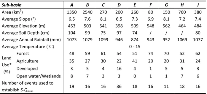
Table 1. Characteristics of nine studied sub-basins and the entire basin

Sub-basin A B C D E F G H J

Area (km2) 1350 2540 270 200 260 80 150 760 380 Average Slope (°) 6.5 7.6 8.1 6.5 7.3 6.9 8.1 7.2 7.4 Average Elevation (m) 453 503 541 398 509 548 562 464 484 Average Soil Depth (cm) 104 99 75 97 74 / / / 80 Average Annual Rainfall (mm) 1073 1079 1099 946 874 943 952 1069 1077

Average Temperature (ºC) 0 - 15 Land Use* (%) Forest 48 59 61 54 51 74 70 52 62 Agriculture 35 27 30 22 41 20 20 31 24 Developed 3 5 4 16 4 1 5 5 3 Open water/Wetlands 8 7 3 3 0 1 1 7 6 Number of events used to

establish S-Qbase

19 16 16 36 18 16 11 18 16

*From National Land Cover Database (NLCD) 2006, zone 63, USGS

Daily stream-flow data were collected at the US Geological Survey (USGS) gauges located at the outlet of each basin (triangles in Fig.2) from 1998 to 2008. Base flow was extracted using the local minimum method, which is automated in the web-based hydrograph analysis tool (WHAT) (Lim et al., 2005). The number of pairs of weather data and stream-flow data for the

(20)

11

nine sub-basins ranges from 11 (basin G) to 36 (basin D) (Refer to appendix for event pairs of nine sub-basins).

Precipitation frequency data were obtained from the website of “Extreme Precipitation in New York and New England” (http://precip.eas.cornell.edu/), which is a joint collaboration between the Northeast Regional Climate Center (NRCC) and the Natural Resources Conservation Service (NRCS) (Refer to appendix for precipitation frequency data for nine sub-basins). The frequency histograms of S were developed based on the “fraction of time” of corresponding Qbase.

Based on the spatial extent of saturated areas predicted by this new method, runoff generating areas within each basin are mapped in a Geographic Information System (GIS) using a Soil Topographic Index (Walter et al. 2002; Lyon et al., 2004).

2.4 Other Considerations

Because the SCS-CN-method does not work well for very small rainfall-runoff events due to the accuracy of rain gauges and the sensitivity of the model (Shaw and Walter, 2009; Buchanan et al., 2011), I only used events associated with daily rainfall higher than 5mm (0.2inch).

(21)

12

Although Ia = 0.2S is a traditional assumption, recent research shows Ia varies for different study areas or events (Jiang, 2001; Shaw and Walter, 2009; Dahlke et al., 2012a). In my calculation, I set Ia = aS, in which a is constant for each basin. I calibrated a so that the least-squares differences between observed and predicted runoff were minimized.

(22)

13

CHAPTER THREE

RESULTS

3.1 Results of Field Test

I first validated my bivariate method with application to the hillslope study site near Ithaca, New York, by comparing the estimated results with observations.

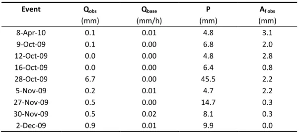
Table 2. Observed rainfall and runoff for the nine storm events

Event Qobs Qbase P Af obs

(mm) (mm/h) (mm) (mm) 8-Apr-10 0.1 0.01 4.8 3.1 9-Oct-09 0.1 0.00 6.8 2.0 12-Oct-09 0.0 0.00 4.8 2.8 16-Oct-09 0.0 0.00 6.4 0.8 28-Oct-09 6.7 0.00 45.5 2.2 5-Nov-09 0.2 0.01 4.7 2.2 27-Nov-09 0.5 0.00 14.7 0.3 30-Nov-09 0.5 0.02 8.1 0.3 2-Dec-09 0.9 0.01 9.9 0.0

Considering the limited available event pairs, I used a “leave-one-out cross-validation” strategy to test my method. Instead of using all nine events, I established the relationship between maximum available soil storage (S) and Qbase for every eight of the nine events. Therefore I obtained nine S-Qbase relationships, which are very similar to each other (Fig. 3).

(23)

14

Figure 3. S versus Qbasefor the study hillslope in central New York State. Two thick black lines are for

the outer bounds of the nine lines.

Based on each established S-Qbaserelationship and the measured Qbase, I estimated S for the corresponding event that was removed. Next, I calculated the fractional saturated areas (Af) from the estimated S and observed P using Eq.2. The predicted Af were then compared with observations. Recognizing that there was one large storm which might have impacted the statistical measures significantly, I plotted the linear regression between predicted Afand observed Af both with the largest storm event included (Fig. 4) and without including the largest storm event (Fig. 4 inset). Though the result without the largest storm event (slope = 0.81, R2 = 0.73) is not as strong as the one for all events (slope = 1.04, R2 = 0.91), the

generally good agreement between estimated and observed Af for both storm histories corroborates my bivariate method for quantifying Af.

(24)

15

I also compared observed Q with Q predicted by the method proposed by Shaw and Walter (2009). The slope of predicted Q versus observed Q is close to 1 and the correlation is high (Fig. 5). The strength of these results, however, is much weaker when the largest event is removed (Fig. 5, insert). Interestingly, the predicted Af results were stronger than the results for Q, which anecdotally suggests the proposed method is not overly sensitive, i.e., Q

measurements were used to derive the relationships in Fig. 3 so one might expect good subsequent model predictions of Q; Af is completely independent of the model

development but still predicted well.

Figure 4. Comparison of predicted saturated areas using a bivariate process and observed saturated areas for the study hillslope in central New York State. Insert shows data pairs for eight storm events excluding the largest storm on 28 October 2009. The lines show the 1:1 relationship.

Af pred= 0.81Af obs+ 0.02 R² = 0.73 0.0 0.1 0.2 0.0 0.1 0.2

(25)

16

Figure 5. Comparison of predicted runoff volumes using the bivariate SCS-CN method (Shaw and Walter, 2009) and observed runoff volumes for the study hillslope in central New York State. Insert shows data pairs for eight storm events excluding the largest storm on 28 October 2009. The lines show the 1:1 relationship.

3.2 Results of Upper Susquehanna Basin Application

I applied the proposed approach to nine sub-basins in Upper Susquehanna River Basin to illustrate predicting risks associated with runoff generating areas as a bivariate process.

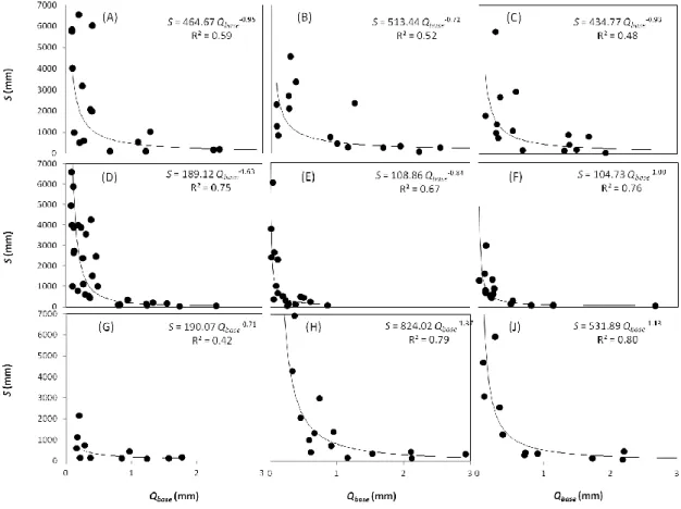
The S-Qbase relationship for each basin were fit by a power function (Fig. 6). Basin J had the highest correlation (R2 = 0.80), while basin G, the one with the least available data, had the lowest correlation (R2 = 0). Qpred= 0.63Qobs+ 0.10 R² = 0.54 0.0 0.5 1.0 0.0 0.5 1.0

(26)

17

Figure 6. S versus Qbase for nine studied sub-basins of the Upper Susquehanna River Basin. The letters correspond to the sub-basins in Table 1. Circles represent pairs of back-calculated S-values from observed P-Q data and base flow immediately preceding the rain event, Qbase; lines are best-fit

power-functions; power functions and associated R2 are shown in each graph.

Based on the S-Qbase relationships, S-valueswere calculated from Qbase for 28 independent storm events (Refer to appendix for Qbase, S, and the corresponding probabilities for the nine sub-basins). Rainfall frequency values obtained from the website of “Extreme Precipitation in New York and New England” (http://precip.eas.cornell.edu/) are plotted in Fig.7. With 7 precipitation values (P) and 28 soil storage values (S), I obtained 196 Af values for each basin. I were then able to estimate bivariate risks associated with Af using Eq.4 (Fig. 8).

(27)

18

Figure 7. Rainfall frequencies for nine studied sub-basins

The fraction of runoff generating areas and the corresponding frequency vary from basin to basin and the trends are distinctly different from the rainfall frequencies (Fig. 7). This

re-emphasizes that the risk associated with a given fraction of a watershed producing runoff does not depend solely on the probability or return period of the causative storm event, but is also influenced by the antecedent soil wetness conditions, which I incorporated in my bivariate approach.

(28)

19

Figure 8. Risks associated with fraction of runoff producing area (Af) for nine studied sub-basins

Based on the S-Qbase relationships, runoff volume Q and the associated runoff risks were determined using the method introduced by Shaw and Walter (2009) (Fig. 9 and Fig. 10).

These results were generated as a reference to the earlier work and for comparison to the

Af risks shown in Fig. 8.

Return period = 2yrs

Af = 18%

Return period = 2yrs

(29)

20

Figure 9. Comparison of predicted runoff volumes using the bivariate SCS-CN method (Shaw and Walter, 2009) and observed runoff volumes for nine studied sub-basins. The events for each basin are the same events previously used to establish power law relationships between S and Qbase.

(30)

21

(31)

22

CHAPTER FOUR

DISCUSSION

4.1 Effects of land uses

The portion of developed area in sub-basin D (16%) is substantially higher than in other watersheds (Table 1). I compared Af risks for sub-basin D to sub-basins C and G, which had much smaller proportions of developed area, 4% and 5%, respectively. All other

characteristics for C, D, and G are relatively similar; C is slightly larger than D, and G is slightly smaller than D (Table 1). For return periods less than ten years, all three

watersheds have similar magnitudes of Af (Fig. 11a) and Q (Fig. 11b). However, when risks become higher (i.e., for larger return periods), the more urbanized or developed sub-basin D has a significantly higher Af and Q. While I expect sub-basin D to have more impervious surfaces than sub-basins C and G, which, logically, will generate storm runoff, it is not immediately obvious to us why the differences appear only at large return periods. However, this is an interesting observation that potentially warrants further study.

(32)

23

Figure 11. Comparisons among sub-basins C, D, and G of risks associated with runoff producing areas (a) and risks associated with runoff volumes (b).

4.2 Mapping the predicted runoff producing areas

In order to apply the relationships between the fraction of runoff generating areas, Af, and the corresponding risks to developing strategies to protect water quality, it is important to map these risks across a watershed. Lyon et al. (2004) proposed using topographic indices

0.0 0.2 0.4 0.6 0.8 1.0 1.2 1 10 100 Af

Return Period (yrs)

C D G 0 10 20 30 40 50 60 70 1 10 100 Q (m m )

Return Period (yrs)

C D G a.

(33)

24

to map Af, and this concept has been adopted by some watershed modelers who use the SCS-CN to predict VSA storm runoff (Agnew et al., 2006; Schneiderman et al., 2007; Easton et al., 2008; Walter et al., 2009; Buchanan et al., 2012). These studies generally used a version of the soil topographic index (STI) proposed for watersheds dominated by shallow restrictive layers, such as those with a fragipan or are shallow depth to bedrock (Walter et al., 2002)

Where a is the upslope contributing area, D is the soil depth above the impervious layer, Ksat is the average soil permeability (or saturated hydraulic conductivity), and tanβ is the local topographic slope. High STI-values indicate areas that have a high propensity of being wet with drier areas having low values of STI.

Runoff risk is mapped as the fractional area of highest STI that corresponds to Af. As an example, the 2-year Af constitutes 18% of sub-basin J (Fig. 8J). This corresponds to an STI of 8.8, or 18% of sub-basin J that has an STI greater than 8.8. The STI and 2-year Af maps for sub-basin J are shown in Fig. 12a and 12b, respectively. This type of information can be used to target parts of the landscape for protection from potentially polluting activities. Unlike previously proposed methods for identifying these sensitive areas, this method combines realistic patterns of runoff generation, in contrast to Gburek et al. (2002) and

(34)

25

considers both the frequency of rainfall and antecedent conditions, in contrast to Walter et al., 2009. The method is relatively simple compared to previously proposed modeling approaches that require decades of simulation modeling (e.g., Walter et al., 2000; 2001; Agnew et al., 2006).

Figure 12. Soil topographic index map (a) and map of “saturated” runoff generating areas associated with a saturation frequency of once every two years (b) for sub-basin J.

While the STI-mapping approach appears to work reasonably well for small to moderate sized watersheds, I experienced two potential problems at the scale of the Upper

Susquehanna Basin: 1) the soil survey data describing soil properties sometimes abruptly changes at county boundaries resulting in un-likely discontinuities in STI. The primary cause of these discontinuities is that the soil depth value for the same map unit being significantly

(35)

26

different in adjacent counties. 2) Valley bottoms generally have very low STI (indicating relatively dry soil conditions) because the accumulated alluvium has a relatively large depth (D) (Fig. 13a); in reality, the effective depth in the valley bottoms should be the water table depth but this is a dynamic characteristic.

An alternative approach is to omit the soil properties from Eq. 4 to calculate a topographic index (TI) (Fig. 13b), which effectively assumes that gravitational redistribution of soil water and groundwater is more important to defining soil wetness patterns than basing these patterns on soil properties derived from soil geographic databases. Valley bottoms appear very different on TI maps compared to STI maps. The TI shows valley bottoms as likely to be wet, i.e., runoff generating, while the STI shows the opposite. The TI probably better

represents spring conditions, when the water table is near the surface and the STI may be more indicative of conditions during the summer and early fall.

(36)

27

Figure 13. Soil topographic index map (a) and topographic index map (b) for the Upper Susquehanna River Basin. Part of the areas in STI map is eliminated due to discontinuities of soil depth data for the same map units that cross county boundaries.

a.

b.

Inconsistent soil survey data

(37)

28

CHAPTER FIVE

SUMMARY AND CONCLUSION

I proposed and demonstrated a bivariate approach that accounts for both rainfall and antecedent soil moisture status within a watershed to improve risk estimates of runoff generating VSAs. My approach effectively combines and extends the previous

re-interpretations of the SCS-CN rainfall-runoff model by Steenhuis et al. (1995), Lyon et al. (2004), and Shaw and Walter (2009). The bivariate method demonstrated good

agreement with the field-measured fraction of runoff-generating areas, considered here as “saturated” areas.

The proposed method provides a potentially useful tool for watershed management to protect water quality from NPS pollution. Mapping the Af associated with a threshold risk level or recurrence interval identifies areas that should be protected from potentially polluting activities. The method described here is potentially simple enough and the computations efficient enough to implement online and/or access via mobile devices.

Some unresolved issues that need more attention include: 1) developing ways to extend risk predictions to ungauged watersheds, 2) resolving problems with discontinuities in soil properties at county boundaries, and 3) determining how to make meaningful predictions for landscapes where a water table effectively limits the soil depth, as opposed to areas where there is a shallow restrictive layer.

(38)

29

APPENDIX

US Geological Survey (USGS) stream gauging station number

Sub-basin A B C D E F G H J

USGS Stream

Gauge Number 1502500 1500500 1500000 1530500 1525981 1521500 1523500 1509000 1510000

National Weather Service (NWS) rain gauging station number

Rain Gauge a b c d e f g

NWS Rain Gauge Number 30770502 30608502 30719502 30867002 30511302 30175202 30261001

Rain Gauge h i j k l m n

NWS Rain Gauge Number 36183806 30477201 30002301 30008501 30398301 30862702 30551202

Observed runoff, baseflow, and rainfall for the nine sub-basins

Sub-basin Event Qobs Qbase P

(mm) (mm) (mm) A 12-Jun-01 0.45 0.38 12.45 17-Jun-01 1.11 0.40 37.85 4-Aug-01 0.58 0.22 13.72 11-Sept-01 0.11 0.10 6.86 14-Sept-01 0.12 0.10 9.91 15-Oct-01 0.12 0.10 11.43 26-Nov-01 0.25 0.14 10.67 24-Jul-02 0.29 0.25 10.67 16-Jul-03 0.43 0.41 12.95 26-Sept-03 0.93 0.68 5.08 25-Nov-03 2.87 2.25 10.67 16-May-04 1.39 1.29 10.16 19-May-04 1.16 1.10 5.59 1-Aug-05 0.21 0.20 6.86 30-Sept-05 0.54 0.27 12.70 2-Nov-05 4.29 3.70 8.89 7-Nov-05 2.67 2.34 7.87 8-Apr-06 1.96 1.22 9.40 24-Nov-06 3.25 3.13 5.84 11-Jul-01 0.40 7 11 15-Oct-01 0.10 10 15 3-Nov-01 0.10 11 3

(39)

30 10-Apr-02 2.13 4 10 24-Jul-02 0.31 0.36 15.24 13-Nov-02 1.66 0.08 10.16 B 12-Apr-03 3.90 0.08 6.86 30-Aug-03 0.60 1.95 8.13 6-Nov-03 2.65 0.26 15.75 20-Nov-03 5.74 1.16 12.45 25-Nov-03 3.14 3.60 5.84 19-May-04 1.11 0.28 44.20 3-Oct-04 1.26 2.55 5.33 23-Jul-05 0.32 1.69 35.56 30-Sept-05 0.20 2.23 8.38 10-Sept-06 0.93 0.99 7.87 C 1-Jun-98 1.38 0.29 28.96 5-Jul-98 2.28 1.29 12.19 7-Jul-99 0.61 0.10 30.73 4-Jul-00 1.38 0.66 11.18 24-Aug-00 0.83 0.56 28.70 4-Sept-00 0.30 0.25 17.27 13-Sept-00 0.94 0.31 41.40 11-Jul-01 0.54 0.26 16.76 10-Apr-02 1.43 1.35 8.38 13-Nov-02 1.85 1.66 12.45 8-Apr-03 4.46 4.11 7.87 8-Jul-03 0.62 0.51 11.18 20-Nov-03 7.88 1.48 38.61 25-Nov-03 3.56 1.91 8.89 23-Jul-05 0.32 0.27 8.64 29-Sept-06 3.76 1.37 32.77 27-Apr-98 1.85 1.34 10.41 30-May-98 0.44 0.39 13.97 1-Jun-98 1.69 0.37 24.89 3-Jun-98 0.69 0.36 13.21 5-Jul-98 2.11 0.83 10.92 16-Sept-98 0.17 0.13 12.70 10-Apr-99 1.68 0.95 15.75 30-Sept-99 0.44 0.12 28.96 14-Oct-99 0.26 0.11 12.19 22-Jun-00 3.01 1.55 15.24 22-Jul-00 0.27 0.23 11.43 7-Aug-00 0.22 0.20 13.97 10-Aug-00 0.41 0.19 13.21 10-Sept-00 0.16 0.14 15.75 18-Oct-00 0.23 0.14 16.26 10-Apr-01 5.56 1.74 10.92 D 17-Jun-01 0.23 0.18 22.86

(40)

31 17-Aug-01 0.16 0.10 27.43 14-Sept-01 0.13 0.08 15.75 15-Oct-01 0.15 0.12 15.24 28-Jun-02 1.93 0.41 48.51 16-Sept-02 0.15 0.10 13.72 23-Sept-02 0.13 0.10 16.00 5-Apr-03 8.02 2.30 18.80 17-May-03 0.63 0.49 11.94 23-Sept-03 1.85 0.30 30.99 26-Apr-04 3.01 1.24 12.45 3-May-04 6.37 1.23 29.21 7-Jun-04 0.39 0.27 11.43 6-Jul-05 0.34 0.19 24.38 10-Nov-05 3.10 0.80 15.75 20-Jun-06 0.40 0.26 18.29 4-Aug-06 0.55 0.31 28.96 10-May-07 0.55 0.47 14.22 19-Jun-07 0.20 0.17 20.83 20-Oct-07 0.15 0.12 12.45 5-Sept-01 0.04 0.02 12.95 14-Sept-01 0.01 0.01 11.94 26-May-02 0.65 0.50 9.14 10-Jul-02 0.10 0.08 6.35 14-Sept-03 0.22 0.19 5.33 16-Sept-03 0.86 0.23 15.49 29-Nov-03 1.77 0.86 9.40 3-May-04 2.47 0.60 23.88 29-Jun-04 0.09 0.06 14.22 E 3-Nov-04 0.86 0.25 6.35 4-Jun-05 0.14 0.11 5.84 7-Jun-05 0.18 0.11 16.51 2-Nov-05 0.55 0.45 7.87 7-Nov-05 0.63 0.38 6.10 11-May-07 2.05 0.28 17.27 9-Jun-07 0.16 0.05 7.11 20-Jun-07 0.05 0.03 20.83 8-Aug-07 0.02 0.01 18.03 5-Sept-01 0.03 0.02 6.10 21-May-03 0.96 0.49 8.38 28-May-03 1.42 0.52 16.51 16-Jul-03 0.20 0.10 16.26 27-Aug-03 0.13 0.12 11.43 30-Aug-03 0.15 0.12 6.35 16-Sept-03 0.71 0.19 18.29 25-Nov-03 1.88 1.13 6.60 28-May-04 5.87 2.67 13.46

(41)

32 F 26-Jun-04 0.29 0.23 7.62 29-Jun-04 0.40 0.20 10.41 11-Aug-04 0.40 0.22 18.54 8-Apr-06 2.10 1.13 8.64 10-Jun-06 0.34 0.24 11.18 20-Jun-06 0.24 0.11 10.92 26-Jul-06 2.87 0.80 12.70 28-May-03 1.42 0.97 14.48 27-Aug-03 0.33 0.20 16.51 30-Aug-03 0.67 0.38 6.60 16-Sept-03 0.62 0.16 16.76 25-Nov-03 1.68 1.24 7.11 G 28-May-04 3.23 1.57 16.00 26-Jun-04 0.36 0.29 7.37 11-Aug-04 0.65 0.17 23.37 8-Apr-06 2.17 1.77 8.64 20-Jun-06 0.49 0.21 6.60 26-Jul-06 1.47 0.85 9.14 1-Jun-98 1.03 0.74 29.72 12-Apr-99 2.40 2.10 11.94 26-Jun-99 0.23 0.21 13.21 11-Nov-99 0.70 0.58 10.92 21-Nov-99 0.74 0.60 7.62 17-Jun-01 0.74 0.45 24.64 1-Sept-01 0.28 0.25 17.78 24-Jul-02 0.52 0.36 33.27 H 17-Aug-03 1.58 1.16 8.89 25-Nov-03 3.33 2.93 12.19 3-Nov-04 0.79 0.66 12.95 2-Nov-05 2.53 2.12 8.13 7-Npv-05 1.70 1.53 8.13 16-May-06 1.03 0.95 10.67 27-May-06 1.95 0.91 28.19 2-Apr-07 4.76 4.32 8.13 24-Apr-07 4.53 3.87 10.92 20-Jun-07 0.72 0.33 41.40 12-Apr-99 1999 4 12 11-Nov-99 1999 11 11 17-Jun-01 2001 6 17 1-Sept-01 2001 9 1 24-Jul-02 2002 7 24 5-Aug-02 2002 8 5 4-Sept-02 2002 9 4 8-Apr-03 2003 4 8 25-Nov-03 2003 11 25 J 3-Nov-04 2004 11 3

(42)

33 2-Nov-05 2005 11 2 7-Nov-05 2005 11 7 27-May-06 2006 5 27 24-Apr-07 2007 4 24 9-Jun-07 2007 6 9 20-Jun-07 2007 6 20

Precipitation frequency data for the nine sub-basins

1 2 5 10 20 50 100 A 53 62 76 88 108 126 148 B 54 64 78 92 113 132 154 C 54 63 78 91 112 132 153 D 50 60 74 87 107 126 148 E 50 59 73 86 106 124 146 F 50 58 71 83 102 120 140 G 50 58 71 83 103 120 141 H 52 60 74 86 106 124 144 J 52 61 75 87 107 125 146

Observed base flow, predicted maximum soil storage capacity, and the corresponding probabilities for the nine sub-basins

Sub-basin Qbase (mm) Spred (mm) Probability (%) 0.12 3491 2.6 0.16 2655 3.7 0.21 2050 3.6 0.26 1673 4.0 0.34 1296 3.7 0.41 1085 3.7 Return Period (yrs) Sub-basin 24-hr Precipitation (mm)

(43)

34 0.47 953 3.1 0.52 865 3.7 0.59 768 3.9 0.67 680 3.1 0.76 603 3.7 0.84 548 3.6 0.92 503 3.7 A 0.99 469 3.5 1.06 440 3.7 1.13 414 3.5 1.21 388 3.7 1.31 359 3.9 1.41 335 3.4 1.52 312 3.3 1.62 294 3.8 1.73 276 3.8 1.88 255 3.7 2.10 229 3.3 2.34 207 3.8 2.67 183 3.5 3.45 143 3.7 7.50 68 3.2 0.08 3203 1.6 0.12 2388 3.4 0.20 1649 2.8 0.30 1229 4.5 0.40 998 4.2 0.50 849 3.1 0.60 744 3.7 0.70 665 3.5 0.80 604 3.9 0.93 541 3.3 1.04 499 3.8 1.16 461 3.6 B 1.26 434 3.4 1.40 402 3.6 1.53 377 2.5

(44)

35 1.54 376 3.4 1.54 375 7.2 1.57 370 3.8 1.61 364 3.3 1.67 354 3.6 1.77 339 3.9 1.89 324 3.9 2.03 307 3.2 2.23 287 3.4 2.50 264 3.7 2.90 237 3.6 4.00 188 3.5 6.60 131 2.5 0.09 4013 3.2 0.11 3398 2.3 0.12 3158 2.3 0.14 2751 6.8 0.20 1993 3.2 0.24 1643 3.6 C 0.29 1364 3.6 0.33 1221 3.5 0.38 1071 3.7 0.46 900 3.6 0.53 785 3.6 0.59 707 3.2 0.65 649 3.9 0.74 576 3.6 0.84 509 3.6 0.92 469 3.5 1.02 427 3.7 1.13 389 3.4 1.23 357 3.6 1.34 332 3.6 1.45 308 3.7 1.59 282 3.5 1.75 258 3.5 1.97 231 3.6

(45)

36 2.20 209 3.6 2.80 167 4.6 6.00 82 5.1 17.30 31 1.1 0.09 9131 2.8 0.10 7853 3.3 0.11 6741 3.8 0.12 6023 3.7 0.13 5155 3.7 0.14 4576 3.7 0.16 3884 3.5 0.18 3194 3.8 0.21 2416 3.5 0.26 1705 3.8 0.29 1427 2.7 0.32 1215 3.8 0.35 1049 3.2 D 0.39 880 3.6 0.44 722 4.0 0.49 606 3.6 0.54 517 4.0 0.58 460 3.6 0.63 402 3.2 0.69 347 4.0 0.75 302 3.4 0.81 267 3.3 0.92 217 3.9 1.03 180 3.6 1.17 146 3.3 1.38 112 3.8 1.74 77 3.4 7.60 7 3.9 0.00 14724 2.3 0.01 6430 4.4 0.02 3580 3.2 0.03 1942 4.3 0.04 1523 3.6

(46)

37 0.06 1224 3.3 0.08 882 3.3 0.11 702 4.1 0.13 606 3.5 0.16 523 3.4 0.19 443 4.0 E 0.22 391 3.3 0.25 351 3.4 0.28 322 3.7 0.31 297 3.7 0.33 278 3.1 0.37 252 3.6 0.41 231 3.7 0.45 214 3.1 0.50 196 3.7 0.55 180 4.1 0.63 161 3.7 0.70 147 3.2 0.81 130 4.0 0.97 112 3.4 1.24 91 4.0 1.68 70 3.5 12.50 13 3.4 0.03 3352 2.2 0.06 1706 6.9 0.08 1318 4.5 0.09 1132 3.8 0.11 965 3.7 0.12 854 3.8 0.14 739 3.5 0.17 617 3.7 0.20 522 3.7 0.23 464 3.3 0.25 413 3.6 0.29 359 3.6 0.33 314 3.7 0.38 275 3.6

(47)

38 0.44 238 3.6 0.49 213 2.5 F 0.50 209 1.3 0.56 187 3.9 0.63 166 3.0 0.71 147 2.9 0.80 131 4.3 0.89 118 4.4 0.96 109 3.2 1.07 98 3.6 1.20 87 3.9 1.50 70 4.2 2.50 42 3.0 9.20 11 2.6 0.08 1210 2.8 0.10 971 3.6 0.12 886 3.3 0.13 817 3.8 0.15 755 4.1 0.16 710 3.5 0.18 647 3.7 0.20 609 3.6 G 0.23 552 3.6 0.25 519 3.8 0.28 476 3.1 0.30 449 3.6 0.34 411 4.0 0.37 387 3.4 0.42 353 3.3 0.49 316 4.2 0.54 295 3.3 0.60 274 3.0 0.67 253 4.2 0.72 240 3.2 0.77 229 3.6 0.84 215 4.6 0.95 197 4.4

(48)

39 1.10 178 4.4 1.22 165 2.7 1.50 142 3.8 2.00 116 3.3 7.50 45 2.1 0.17 9238 2.6 0.22 6589 3.1 0.25 5528 3.7 0.30 4304 4.7 0.34 3624 3.7 0.39 3002 3.0 0.46 2393 4.1 0.52 2022 3.5 0.59 1700 3.4 0.64 1521 3.7 0.71 1319 3.9 0.79 1139 3.4 0.89 967 3.8 H 0.98 847 3.4 1.06 761 3.2 1.13 697 3.6 1.24 613 4.0 1.35 546 3.7 1.44 499 3.5 1.57 444 3.5 1.68 404 3.6 1.83 359 4.0 1.99 320 3.9 2.18 283 3.4 2.42 245 3.4 2.85 196 3.7 3.60 142 3.3 16.00 18 3.3 0.08 8878 2.5 0.12 5851 3.4 0.16 4226 3.8 0.21 3107 4.2

(49)

40 0.26 2440 3.5 0.33 1864 4.0 0.39 1543 3.5 0.47 1249 3.7 0.53 1091 3.3 0.60 948 3.5 0.67 837 3.4 J 0.75 736 4.2 0.82 666 3.0 0.90 599 4.3 0.99 538 3.4 1.10 478 3.6 1.21 429 3.6 1.31 392 3.4 1.41 361 3.5 1.52 331 3.8 1.65 302 3.8 1.80 274 3.9 1.96 248 3.7 2.17 221 3.6 2.50 189 3.7 3.10 148 3.7 4.50 97 3.6 18.00 20 2.5

(50)

41

REFERENCES

Agnew L.J., Lyon S., Gérard-Marchant P., Collins V.B., Lembo A.J., Steenhuis T.S., Walter M.T. 2006. Identifying hydrologically sensitive areas: Bridging the gap between science and application. Journal of environmental management 78 : 63-76.

Brutsaert W. 1993. Effective water table depth to describe initial conditions prior to storm rainfall in humid regions. Water Resour.Res 29 : 427-34.

Buchanan, B.P., Z.M. Easton, R.L. Schneider, M.T. Walter. 2012. Incorporating variable source area hydrology into a spatially distributed storm runoff model. Journal of the American Water Resources Association (in press).

Dahlke H.E., Easton Z.M., Lyon S.W., Todd Walter M., Destouni G., Steenhuis T.S. 2012a. Dissecting the variable source area concept–Subsurface flow pathways and water mixing processes in a hillslope. Journal of Hydrology, 420–421: 125–141.

Dahlke, H.E., Z.M. Easton, M.T. Walter, T.S.Steenhuis. 2012b. A field test of the variable source area interpretation of the Curve Number rainfall-runoff equation. ASCE Journal of Irrigation and Drainage

(in press).

Dunne T., Black R.D. 1970. Partial area contributions to storm runoff in a small New England watershed. Water Resources Research 6 : 1296-311.

Easton, Z.M., D.R. Fuka, M.T. Walter, D.M. Cowan, E.M. Schneiderman, T.S. Steenhuis. 2008. Re-conceptualizing the Soil and Water Assessment Tool (SWAT) model to predict saturation excess runoff from variable source areas. Journal of Hydrology348(3-4): 279-291.

Fiorentino M., Iacobellis V. 2001. New insights about the climatic and geologic control on the probability distribution of floods. Water Resources Research 37 : 721-30.

Frankenberger J.R., Brooks E.S., Walter M.T., Walter M.F., Steenhuis T.S. 1999. A GIS-based variable source area hydrology model. Hydrological Processes 13 : 805-22.

Fry J.A. 2011. Completion of the 2006 National Land Cover Database for the Conterminous United

States. Photogrammetric Engineering and Remote Sensing 77 : 858.

Garen D.C., Moore D.S. 2005. Curve Number hydrology in water quality modeling: Uses, abuses, and future directions. Journal of the American Water Resources Association (JAWRA) 41 : 377-88.

(51)

42

Gburek W., Drungil C., Srinivasan M., Needelman B., Woodward D. 2002. Variable-source-area controls on phosphorus transport: Bridging the gap between research and design. Journal of Soil and Water Conservation 57 : 534.

Horton R.E. 1933. The role of infiltration in the hydrologic cycle. Trans.Am.Geophys.Union 14 : 446-60.

Horton R.E. 1940. An approach toward a physical interpretation of infiltration capacity. 5 : 24. Jiang, R. 2001. Investigation of Runoff Curve Number Initial Abstraction Ratio, M.S. thesis, Univ. of Ariz., Tucson.

Lim K.J., Engel B.A., Tang Z., Choi J., Kim K.S., Muthukrishnan S., Tripathy D. 2005. Automated Web Gis Based Hydrograph Analysis Tool, What1. JAWRA Journal of the American Water Resources Association 41 : 1407-16.

Lyon S.W., Walter M.T., Gérard‐Marchant P., Steenhuis T.S. 2004. Using a topographic index to distribute variable source area runoff predicted with the SCS curve‐number equation. Hydrological Processes 18 : 2757-71.

Lyon S.W., Lembo A.J. 2006a. Defining probability of saturation with indicator kriging on hard and soft data. Advances in Water Resources 29 : 181-93.

Lyon S., Seibert J., Lembo A., Walter M., Steenhuis T. 2006b. Geostatistical investigation into the temporal evolution of spatial structure in a shallow water table. Hydrology and Earth System Sciences 10 : 113-25. McCuen R.H. 2002. Approach to confidence interval estimation for curve numbers. Journal of Hydrologic Engineering 7 : 43.

Macrae M., English M., Schiff S., Stone M. 2010. Influence of antecedent hydrologic conditions on patterns of hydrochemical export from a first-order agricultural watershed in Southern Ontario, Canada. Journal of Hydrology 389 : 101-10.

McCuen R.H. 2002. Approach to confidence interval estimation for curve numbers. Journal of Hydrologic Engineering 7 : 43.

Michele C.D., Salvadori G. 2002. On the derived flood frequency distribution: analytical formulation and the influence of antecedent soil moisture condition. Journal of Hydrology 262 : 245-58. Mishra S.K., Singh V.P. 2006. A relook at NEH‐4 curve number data and antecedent moisture

condition criteria. Hydrological Processes 20 : 2755-68. Ponce V.M., Hawkins R.H. 1996. Runoff curve number: Has it reached maturity? Journal of Hydrologic Engineering 1 : 11-9.

(52)

43

Shaw S.B., Walter M.T. 2009. Improving runoff risk estimates: Formulating runoff as a bivariate process using the SCS curve number method. Water Resources Research 45 : W03404.

Shaw S.B., Riha S.J. 2011. Assessing possible changes in flood frequency due to climate change in mid‐sized watersheds in New York State, USA. Hydrological Processes .

Schneiderman, E.M., T.S. Steenhuis, D.J. Thongs, Z.M. Easton, M.S. Zion, A.L. Neal, G.F. Mendoza, M.T. Walter. 2007. Incorporating variable source area hydrology into Curve Number based watershed loading functions. Hydrological Processes21(25): 3420-3430.

Steenhuis T.S., Winchell M., Rossing J., Zollweg J.A., Walter M.F. 1995. SCS runoff equation revisited for variable-source runoff areas. Journal of Irrigation and Drainage Engineering 121 : 234-8. U.S. Soil Conservation Service (SCS). 1972. Hydrology, in National Engineering Handbook, U.S. Gov. Print. Off., Washington, D.C.

Walter M.T., Walter M.F., Brooks E.S., Steenhuis T.S., Boll J., Weiler K. 2000. Hydrologically sensitive areas: Variable source area hydrology implications for water quality risk assessment. Journal of Soil and Water Conservation 55 : 277.

Walter M.T., Brooks E., Walter M.F., Steenhuis T.S., Scott C., Boll J. 2001. Evaluation of soluble phosphorus loading from manure-applied fields under various spreading strategies. Journal of Soil and Water Conservation 56 : 329-35.

Walter M.T., Steenhuis T.S., Mehta V.K., Thongs D., Zion M., Schneiderman E. 2002. Refined

conceptualization of TOPMODEL for shallow subsurface flows. Hydrological Processes 16 : 2041-6. Walter M.T., Mehta V.K., Marrone A.M., Boll J., Gérard-Marchant P., Steenhuis T.S. 2003. Simple estimation of prevalence of Hortonian flow in New York City watersheds. Journal of Hydrologic Engineering 8 : 214.

Walter M.T., Shaw S.B. 2005. DISCUSSION1. JAWRA Journal of the American Water Resources Association 41 : 1491-2.

Walter T., Dosskey M., Khanna M., Miller J., Tomer M., Wiens J. 2007. The science of targeting within landscapes and watersheds to improve conservation effectiveness. Soil and Water : 63-89.

Walter M.T., Archibald J.A., Buchanan B., Dahlke H., Easton Z.M., Marjerison R.D., Sharma A.N., Shaw S.B. 2009. New paradigm for sizing riparian buffers to reduce risks of polluted storm water: practical synthesis. Journal of Irrigation and Drainage Engineering 135 : 200.

Ward R.C. 1984. On the response to precipitation of headwater streams in humid areas. Journal of Hydrology 74 : 171-89.