H
i-S
ta
t
D
is
cu
ss
io
n
P
a
p
er
Research Unit for Statistical
and Empirical Analysis in Social Sciences (Hi-Stat)
Hi-Stat
Institute of Economic Research Hitotsubashi University 2-1 Naka, Kunitatchi Tokyo, 186-8601 JapanGlobal COE Hi-Stat Discussion Paper Series
Research Unit for Statistical
and Empirical Analysis in Social Sciences (Hi-Stat)
December 2010
Nonparametric Quantile Regression with
Heavy-Tailed and Strongly Dependent Errors
Toshio Honda
157
Nonparametric Quantile Regression with Heavy-Tailed
and Strongly Dependent Errors
Toshio Honda∗
Graduate School of Economics, Hitotsubashi University, Tokyo 186-8601, JAPAN
Abstract
We consider nonparametric estimation of the conditional qth quantile for stationary time series. We deal with stationary time series with strong time dependence and heavy tails under the setting of random design. We estimate the conditional qth quantile by local linear regression and investigate the asymptotic properties. It is shown that the asymptotic properties are affected by both the time dependence and the tail index of the errors. The results of a small simulation study are also given.
Key words: conditional quantile, random design, check function, local linear regression, stable distribution, linear process, long-range dependence, martingale central limit theorem
1. Introduction
Let{(Xi, Yi)} be a bivariate stationary process generated by
Yi =u(Xi) +Vi, i= 1,2, . . . , (1) where Vi = V(Xi, Zi), Xi = J(. . . , ϵi−1, ϵi), Zi =
∑∞
j=0cjζi−j, and {ϵi} and {ζi} are mutually independent i.i.d. processes. Then we estimate the qth conditional quantile of Yi given Xi = x0 from n observations by appealing
to local linear regression and investigate the asymptotic properties of the estimator.
We adopt the DGP and the dependence measure of Wu et al. (2010), which allows us to consider nonlinearity and long-range dependence (LRD).
We can also deal with {Xi} that does not satisfy α-mixing conditions suf-ficient for the central limit theorem. See Wu et al.(2010) for the details. Assuming that {Zi}is a heavy-tailed linear process andcj does not decay so fast, we examine how the heavy tail and the time dependence through {cj}
affect the asymptotic properties of the local linear estimator in the setting of (1). We need the assumption of linear process as in (1) to derive the asymptotic distribution of the estimator.
We state a few assumptions onu(x) and V(x, z) here. Let u(x) be twice continuously differentiable in a neighborhood ofx0. We denote theqth
quan-tile of Z1 by mq and assume that V(x, z) is monotone increasing in z and
V(x, mq) = 0 for any x. Then u(x0) is the conditional qth quantile given
Xi = x0. An example of V(x, z) is σ(x)(z −mq). Some more technical assumptions on V(x, z) will be given in section 2.
There have been a lot of studies on quantile regression for linear models since Koenker and Basset (1978). It is because quantile regression gives us more information about data than mean regression and is robust to outliers. Pollard (1991) devised a simple proof of the asymptotic normality of regres-sion coefficient estimators. See Koenker (2005) for recent developments of quantile regression.
We often employ nonparametric regression when we have no parametric regression function or when we want to check the parametric regression func-tion. Chaudhuri (1991) considered nonparametric estimation of conditional quantiles for i.i.d observations and Fan et al. (1994) applied the method of Pollard (1991) to nonparametric robust estimation including nonparametric estimation of conditional quantiles. We examine the estimator of Chaudhuri (1991) in our setting by exploiting the method of Pollard (1991). See Fan and Gijbels (1996) for nonparametric regression and local linear estimators. Many authors have considered cases of weakly dependent observations and studied the asymptotic properties of the nonparametric quantile estima-tors since Chaudhuri (1991). For example, Truong and Stone (1992) con-sidered local medians for α-mixing processes. Honda (2000a) and Hall et al.(2002) examined the asymptotic properties of the estimator of Chaudhuri (1991). Hall et al.(2002) also employed the method of Pollard (1991) for
α-mixing processes. Zhao and Wu (2006) considered another setting from
α-mixing processes. The above authors considered nonparametric quantile estimation under random design. Zhou (2010) is a recent paper for nonpara-metric quantile estimation under fixed design. See Fan and Yao (2003) for nonparametric regression for time series.
Some authors investigated robust or nonparametric estimation of regres-sion functions for LRD time series with finite variance after the developments of theoretical results on time series with LRD, especially, the results on lin-ear processes by Ho and Hsing (1996,1997). Giraitis et al. (1996) deals with robust linear regression under LRD. See Robinson (1997), Hidalgo (1997), Cs¨org˝o and Mielniczuk (2000), Mielniczuk and Wu (2004), and Guo and Koul (2007) for nonparametric estimation of conditional mean functions. Wu and Mielniczuk (2002) fully examined the asymptotic properties of kernel den-sity estimators. Wu et al. (2010) also deals with kernel denden-sity estimation and nonparametric regression and the results are useful to the present pa-per. Honda (2000b) and Honda (2010) considered nonparametric estimation of conditional quantiles when {Xi} and {Zi} are LRD linear processes with finite variance in (1). It is now known that the asymptotic distributions of nonparametric estimators drastically change depending on the strength of dependence and the bandwidths in the cases of density estimation and nonparametric regression under random design. The time dependence of covariates has almost no effect on the asymptoitics except for technical con-ditions in the setting similar to (1). See Beran (1994), Robinson (2003), and Doukhan et al.(2003) for surveys on time series with LRD.
Following Ho and Hsing (1996,1997), Hsing (1999), Koul and Surgailis (2001), Surgailis (2002), Pipiras and Taqqu (2003), and Honda (2009b) stud-ied the limiting distributions of partial sums of bounded functionals of LRD linear processes with infinite variance. We state Assumptions Z1-2 on {Zi}
to describe their results. Let an∼a′n mean an/a′n →1 as n→ ∞. Assumption Z1: cj ∼czj−β and c0 = 1.
Assumption Z2: Write G0(z) for the distribution function of ζ1. Then
there exists 0< α <2 s.t. lim z→−∞|z| α G0(z) = c− and lim z→∞|z| α (1−G0(z)) =c+,
where c−+c+ >0. In addition, E{ζ1}= 0 when α >1.
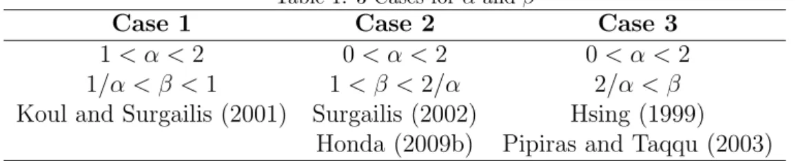
Hereafter we assume that Assumptions Z1-2 hold. Then there are three Cases in the literature and we summarize the cases and the references in Table 1 below. Some authors say that the linear process has LRD in Cases 1-2. Note that ζ1 belongs to the domain of attraction of the α-stable distribution
Sα(σ, η, µ), whose characteristic function is given by
{
exp{−σα|θ|α(1−iηsign(θ) tan(πα/2)) + iµθ} for α̸= 1,
Table 1: 3 Cases forαandβ
Case 1 Case 2 Case 3 1< α <2 0< α <2 0< α <2 1/α < β <1 1< β <2/α 2/α < β
Koul and Surgailis (2001) Surgailis (2002) Hsing (1999) Honda (2009b) Pipiras and Taqqu (2003)
where 0 < σ, −1 ≤ η ≤ 1, −∞ < µ < ∞, and i stands for the imaginary unit. See Samorodnitsky and Taqqu (1994) for more details about stable distributions. In Case 3, we have 1 √ n n ∑ i=1 (H(Zi)−E{H(Zi)}) d →N(0, σ2),
where→d denotes convergence in distribution andH(z) is a bounded function. In Cases 1 and 2, the limiting distribution is anα- andαβ-stable distribution with n−1+β−1/α and n−1/(αβ) as the normalization constant, respectively.
Some authors have considered robust parametric or nonparametric esti-mation under dependent errors with infinite variance, i.e. in Case1, Case2 with α > 1, and Case 3. Peng and Yao (2004) and Chan and Zhang (2009) considered robust nonparametric regression under fixed design. Honda (2009a) considered kernel density estimation by following Wu and Mielniczuk (2002) and found that the asymptotic distributions depend on α and β in Assumptions Z1-2. Koul and Surgalis (2001) and Zhou and Wu (2010) deals with linear regression in Case 1.
In this paper, we consider nonparametric estimation of the conditional
qth quantile in (1) in Cases 1-3 by following Honda (2010). We can also say that this paper is a random-design version of Peng and Yao (2004) and Chan and Zhang (2009). Then we find thatαandβaffect the asymptotics in Cases 1-2 and that we have the same asymptotics as for i.i.d. observations in Case 3. We also conclude that the time dependence of {Xi} has almost no effect on the asymptotics in Cases 1 and 3. The Case 2 is the most challenging and we have not resolved the effect of the LRD of{Xi}completely. See Theorem
2 below for more details. We conjecture that the strong LRD of {Xi} affects the asymptotics of the estimator. However, this is a topic of future research. This paper is organized as follows. In Section 2, we describe assumptions, define the local linear estimator, and present the asymptotic properties in Theorems 1-3. We carried out a small simulation study and the results are reported in Section 3. We state Propositions 1-5 and prove Theorems 1-3 in Section 4. All the technical details are confined to Sections 5-6.
Finally in this section, we introduce some notation. We write|w| andAT for the Euclidean norm of a vector w and the transpose of a matrix A. We denote the Lp norm of a random variableW by∥W∥p and pis omitted when
p = 2. Let →p denote convergence in probability and we omit a.s. (almost surely) when it is clear from the context.
We writea∧b and a∨b for min{a, b} and max{a, b}, respectively. LetR and Zdenote the set of real numbers and integers, respectively. Throughout this paper, C and δ are positive generic constants and the values vary from place to place. The range of integration is also omitted when it is R.
2. Local linear estimator and asymptotic properties
We state assumptions, define the local linear estimator, and present the asymptotic properties of the estimator in Theorems 1-3.
First we state Assumption V onV(x, z). Recall thatmqis theqth quantile of Z1
Assumption V: V(x, z) is monotone increasing in z and V(x, mq) = 0 for any x. Besides, V(x, z) is continuously differentiable in a neighborhood of (x0, mq) and ∂V(x0, mq)/∂z >0.
We need a kernel function K(ξ) and a bandwidth h to define the local linear estimator.
Assumption K: The kernel function K(ξ) is a symmetric and bounded density function with compact support [−CK, CK]. We write κj and νj for
∫
ξjK(ξ)dξ and ∫ ξjK2(ξ)dξ, respectively.
Assumption H: h=chn−1/5 for some positive ch.
We impose Assumption H for simplicity of presentation. However, other choices of h do not improve the rate of convergence of the estimator. There is no theoretical difficulty in dealing with the case where Xi ∈Rd. Then we should take h=chn−1/(d+4).
Now we introduce the check function ρq(u) and the derivative ρ′q(u) in (2) to define the local linear estimator of u(x0).
ρq(u) =u(q−I(u <0)) and ρ′q(u) =q−I(u <0). (2) Then we estimate (u(x0), hu′(x0))T by ˆ β = ( ˆβ1,βˆ2)T = argminβ∈R2 n ∑ i=1 Kiρq(Yi−ηiTβ), where Ki =K((Xi−x0)/h) and ηi = (1,(Xi−x0)/h)T.
We normalize ˆβ−(u(x0), hu′(x0))T byτn and define ˆθ by ˆ
θ=τn( ˆβ1−u(x0),βˆ2−hu′(x0))T. (3)
We specify τn later in this section. It is easy to see that ˆθ is also defined by
ˆ θ= argminθ∈R2 n ∑ i=1 Kiρq(Vi∗−τ− 1 n η T i θ), (4) where Vi∗ =V(Xi, Zi) + 1 2 (X i−x0 h )2 u′′( ¯Xi) and ¯Xi is betweenx0 and Xi.
Before stating assumptions on {Xi} and {Zi}, we define σ-fields Fi, Gi, and Si by
Fi =σ(. . . , ϵi−1, ϵi), Gi =σ(. . . , ζi−1, ζi), Si =σ(. . . , ϵi−1, ζi−1, ϵi, ζi). We adopt the setup and the notation of Wu et al.(2010), especially that of subsection 2.1, for {Xi} and Assumption X1 below is necessary to define the dependence measure.
Set
Fl(x|Fi) = P(Xi+l ≤x|Fi). (5) Assumption X1: With probability 1, F1(x|F0) is differentiable on R and
the derivativef1(x|F0) satisfies supRf1(x|F0)≤Cand limx→x0E{|f1(x|F0)−
f1(x0|F0)|}= 0.
We write f(x) for the density function of X1 and assume that f(x0)>0
Another σ-field Fi∗ below is used to define the dependence measure of {Xi} as in Wu et al.(2010). F∗ i = { σ(. . . , ϵ−1, ϵ∗0, ϵ1, . . . , ϵi) for i≥0, Fi for i <0,
whereϵ∗0 is an independent copy ofϵ0. Define the dependence measureθj,p(x) by
θj,p(x) =∥f1+j(x|F0)−f1+j(x|F0∗)∥p.
for p > 1 andj ≥0. When j <0, set θj,p(x) = 0. Then we have
∥E{f1(x|Fi)|Fi−j} −E{f1(x|Fi)|Fi−j−1}∥p ≤θj,p(x). (6) We also define p′, θp(j), and Θp byp′ = 2∧p,
θp(j) = sup x∈R θj,p(x), and Θp(n) = ∑ i∈Z ( n−i ∑ j=1−i θp(j))p ′ . (7)
We find in Subsection 4.1 of Wu et al.(2010) thatθp(j)≤C|bj|for 1< p≤2 when E{|ϵi|2}<∞ and X i is given by Xi = ∞ ∑ j=0 bjϵi−j. (8) Assumption X2: (Θp(n))1/p ′ /n →0 for some 1 < p.
Assumption X2 will be employed to deal with ∑ni=1(f1(x0 +ξh|Fi−1)−
f(x0+ξh)). In fact, Lemma 3 of Wu et al.(2010) implies that
sup x∈R ∥ n ∑ i=1 (f1(x|Fi−1)−f(x))∥p ≤C(Θp(n))1/p ′ (9) and that almost every linear process with finite variance satisfies Assumption X2. We assume that Assumptions X1-2 hold throughout the paper.
Assumptions X3-5 below will be used to derive the asymptotic distribu-tion when the effects of α and β appear in the asymptotics.
Assumption X3: ∑∞j=1θp(j)<∞.
Assumption X3 means that {Xi} has short-range dependence (SRD). It is easy to see that Assumption X3 implies Assumption X2. We take p = α
Hereafter we writeAξ(i) forf1(x0+ξh|Fi−1) for notational convenience.
Recall that E{Aξ(i)} = f(x0 +ξh). Assumption X4 below holds under (8)
withbj ∼cXj−(1+δ1)/2 and E{|ϵ1|2+δ2}<∞for some positiveδ1andδ2. Thus
it is just a mild assumption and will be used in Case 1. Assumption X4: There exists a positive γx s.t.
|Cov(Aξ(i), Aξ(j))| ≤C|i−j|−γx for i̸=j.
Assumption X5: There exist rx and δx s.t. αβ < rx, δx >0, and θrx(j)≤
Cj−δx−1/(αβ) .
Assumption X5 will be used in Case 2. The assumption is rather restric-tive because it depends on αβ. However, it seems very difficult to derive the asymptotic distribution without this kind of assumption when we see the effects of α and β. See a comment on this difficulty around (11) and (12) below.
We introduce some more notation to state another assumption on {Zi}. We define Zi,j and ˜Zi,j by
Zi,j = j
∑
l=0
clζi−l and Z˜i,j =Zi−Zi,j = ∞
∑
l=j+1
clζi−l
and let Gj(z) denote the distribution function of Z1,j. Then G∞(z) is that of Z1.
Assumption Z3: There exists a positive γz s.t. for any j,
|G′′j(z)| ≤C(1 +|z|)−(1+γz) and |G′′ j(z1)−G′′j(z2)| ≤ C|z1 −z2| (1 +|z1|)(1+γz) (10) for |z1−z2| ≤1. In addition, g∞(mq)>0.
Assumption Z3 is a technical one and Lemma 4.2 of Koul and Surgailis (2001) implies that Assumption Z3 can be relaxed for α > 1. When ζ1 has
a stable distribution, Assumption Z3 follows from the argument based on integration by parts in Hsing (1999).
We divide Case 1 into Cases 1A and 1B and Case 2 into Cases 2A-C, respectively to present Theorems 1-3. We also specify the normalization constant τn for each case here.
Case 1: 1< α <2, 1 < αβ <2, and β <1 Case 1A: 1/α−β <−2/5 and τn =
√
Case 1B: 1/α−β > −2/5 and τn = nβ−1/α. In addition, Assumption X3 with p=α or X4 holds.
Case 2: 0< α <2, 1 < αβ <2, and β >1 Case 2A: 1/(αβ)<3/5 and τn=
√
nh.
Case 2B: 1/(αβ)>3/5 and τn=nν, where ν <1−1/(αβ).
Case 2C:1/(αβ)>3/5 and τn =n1−1/(αβ). In addition, Assumption X3 with αβ < p or X5 holds.
Case 3: αβ >2 and τn = √
nh.
In Cases 1A, 2A, and 3, we have the same asymptotic distribution as for i.i.d. observations. On the other hand, we see the effects of α and β in Cases 1B, 2B, and 2C and have worse convergence rates. We have to impose additional assumptions on{Xi}to investigate the asymptotic distribution of the nonparametric quantile estimator in those cases. Especially in Case 2, we have to show n−1/(αβ) n ∑ i=1 (Aξ(i)−E{Aξ(i)})B1( ˜Zi,0) = op(1) (11) or to deal with n−1/(αβ) n ∑ i=1 ∞ ∑ j=1 Aξ(i+j)(Bj(cjζi)−E{Bj(cjζi)}), (12) whereBj(z) is specified later in Proposition 2. We will prove (11) and derive the asymptotic distribution in Case 2C. When (11) does not seem to hold, we have to deal with (12). However, Aξ(i+j) in (12), not Aξ(i), will extremely complicate the theoretical treatment and we do not pursue the problem in this paper.
Theorems 1-3 below deals with Cases 1-3, respectively. We denote the density of V(x0, Z1) by fV(0|x0), which is written as
fV(0|x0) = g∞(mq)
(∂V
∂z (x0, mq)
)−1
.
Theorem 1. Suppose that Assumptions V, K, H, Z1-3, and X1-2 hold in Case 1. In Case 1B, Assumption X3 with p = α or X4 is also assumed. Then we have as n→ ∞,
Case 1A: ˆ θ →d N (( c5h/2u′′(x0)κ2 2 0 ) , q(1−q) f2 V(0|x0)f(x0) ( ν0 0 0 κ−22ν2 )) , Case 1B: ˆ θ = − 1 fV(0|x0) ( 1 0 ) ∫ ρ′q(V(x0, z))g∞′ (z)dz τn n n ∑ i=1 ˜ Zi,0+op(1) d → − 1 fV(0|x0) ( 1 0 ) ∫ ρ′q(V(x0, z))g∞′ (z)dzcdL, where ∫ ρ′q(V(x0, z))g∞′ (z)dz =−g∞(mq), L∼Sα(1,(c+−c−)/(c++c−),0), and cd=cz ( (c++c−) Γ(2−α) cos(απ/2) 1−α ∫ 1 −∞ { ∫ 1 0 (t−s)−+βdt } ds )1/α .
Theorem 2. Suppose that Assumptions V, K, H, Z1-3, and X1-2 hold in Case 2. In Case 2C, Assumption X3 with αβ < p or X5 is also assumed. Then we have as n→ ∞,
Case 2A: we have the same result as in Case 1A, Case 2B: θˆ=op(1), Case 2C: ˆ θ→d σαβ fV(0|x0) ( 1 0 ) (c1+/(αβ)Cq+L++c1−/(αβ)Cq−L−), where L+ ∼ S
αβ(1,1,0), L− ∼ Sαβ(1,1,0), L+ and L− are mutually inde-pendent, σαβ = {cα zΓ(2−αβ)|cos(παβ/2)| (αβ−1)βαβ }1/(αβ) , Cq± = ∫ ∞ 0 (q−G∞(mq∓v)v−(1+1/β)dv.
In Case 2B, we have only proved that ˆβ−(u(x0), hu′(x0))T =op(n−ν) for any ν < 1−1/(αβ).
Theorem 3. Suppose that Assumptions V, K, H, Z1-3, and X1-2 hold in Case 3. Then we have the same result as in Case 1A.
Theorems 1-2 shows that the asymptotic properties may be badly affected by α and β in Cases 1B, 2B, and 2C. Generally speaking, the convergence rates of mean regression are worse than those of quantile regression when
α < 2. However, the convergence rate is the same as that of nonparametric mean regression in Case 1B. In Case 2, the rates are improved and better than n−1+1/α.
In Section 3, we report the results of our simulation study to show how
α and β affect the properties of the local linear estimator.
In Cases 1A, 2A, and 3, our choice ofhin Assumption H gives the optimal rate of convergence to the local linear estimator. In Cases 1B and 2C, the rate of convergence is independent of h and any other choices of h does not improve the rate. Therefore we recommend that we should choose the bandwidth as if we had i.i.d. observations.
The asymptotic distribution depends onα andβ in a complicated way in Cases 1B and 2C. It might be very difficult to estimate the parameters and statistical inference is a topic of future research.
3. Simulation study
We carried out a small simulation study by using R. In the simulation study, ϵi ∼N(0,1), ηi ∼Sα(1,0,0), Yi = 2(Xi2+X 4 i) +Zi, Xi = 999 ∑ j=0 cx (1 +j)γϵi−j, Zi = 999 ∑ j=0 cz (1 +j)βηi−j, where cx and cz are chosen so that Xi ∼N(0,1) and Zi ∼Sα(1,0,0).
We took γ = 0.75, 1.25, x0 = 0.0, 0.6, and h = 0.2, 0.4. We examined
20 pairs of (α, β), α = 1.1, 1.2, 1.3, 1.4, 1.5 and β = 0.9, 1.3, 1.7, ∞. The sample size is 400 and the results are based on 10,000 repetitions.
We estimate u(x0) by employing the rq function of the quantreg
pack-age(Koenker (2009)) with the Epanechnikov kernel and use the rstable func-tion of the fBasics package(Wuertz et al.(2009)) to generate Sα(1,0,0) ran-dom numbers. When there are less than four observations available to es-timate u(x0), just the sample median is used here. However, there are less
than 10 of the repetitions for each entry of Tables 2-6 below and there will be almost no influence on the results.
Tables 2-6 are for the cases of α = 1.1, 1.2, 1.3, 1.4, 1.5, respectively in the case of γ = 0.75. Tables 7-11 are for the same pairs with γ = 1.25. Note
that all of (∗,0.9) belong to Case 1B. Pairs (1.1,1.3) and (1.2,1.3) belong to Cases 2B and 2C in the cases of γ = 0.75 and γ = 1.25, respectively. The other pairs have the same asymptotic distribution as for i.i.d. observations. In the tables, every entry is estimated by the sample mean. “mean” is the mean of ˆβ1 and “bias” is the mean minus the true value. “mse” is the mean
squared error and N/A means that the MSE does exist from a theoretical point of view. Actually, we had unstable and extremely large values. Values with∗in the tables were unstable and the true values may not exist. “madev” stands for the mean absolute deviation, E{|βˆ1−u(x0)|}.
Tables 2-11 are around here.
We have the following observations from Tables 2-11.
1. In the cases ofβ = 0.9, the values of madv are very large for small α. This implies that the effects of small β and small α are very serious and that nonparametric estimation may be very difficult.
2. In the cases ofβ = 1.3, the values of mse are large forα= 1.3−1.5. We should have the same asymptotic distribution as for i.i.d. observations in those cases. The values of madv are still larger than those forβ =∞. 3. In the cases of β = 1.7, the effects of small α on mse are serious up to
α= 1.3 and the madv values are also severely affected up toα = 1.2. 4. There are not large differences in the mean absolute deviation between
γ = 0.75 and γ = 1.25. But there may be a difference in the MSE in (1.2,1.7).
5. Larger bandwidths yield better results for the MSE. But there is almost no difference in the mean absolute deviation between h = 0.2 and
h= 0.4 .
The effects of α and β are serious and there seem to be considerable differences between the asymptotics and the finite sample properties.
4. Proofs of Theorems 1-3
We verify Theorems 1-3 in a similar way to Theorem 1 of Honda (2010). Honda (2010) deals with linear process with finite variance. First we state Propositions 5, which are essential tools to the proofs. Propositions 1-3 deal with the stochastic term of the estimator and they correspond to
Lemma 1 of Honda (2010). Propositions 4 and 5 correspond to Lemmas 2 and 3, respectively and deal with all the cases at the same time. Proposition 5 is related to the bias term.
Proposition 1. Suppose that the same assumptions hold as in Theorem 1. Then we have as n→ ∞, Case 1A: τn nh n ∑ i=1 Kiηiρ′q(Vi) d →N (( 0 0 ) , q(1−q)f(x0) ( ν0 0 0 ν2 )) , Case 1B: τn nh n ∑ i=1 Kiηiρ′q(Vi) = −f(x0) ( 1 0 ) ∫ ρ′q(V(x0, z))g∞′ (z)dz· τn n n ∑ i=1 ˜ Zi,0 +op(1) d → −f(x0) ( 1 0 ) ∫ ρ′q(V(x0, z))g∞′ (z)dz·cdL, where cd and L are defined in Theorem 1.
Proposition 2. Suppose that the same assumptions hold as in Theorem 2. Then we have as n→ ∞,
Case 2A: we have the same result as in Case 1A of Proposition 1, Case 2B: τn nh ∑n i=1Kiηiρq′(Vi) = op(1), Case 2C: τn nh n ∑ i=1 Kiηiρ′q(Vi) d →f(x0) ( 1 0 ) σαβ(c 1/(αβ) + Cq+L ++c1/(αβ) − Cq−L−), where σαβ, Cq±, and L± are defined in Theorem 2.
Proposition 3. Suppose that the same assumptions hold as in Theorem 3. Then we have the same result as in Case 1A of Proposition 1.
Proposition 4. Suppose that the Assumptions V, K, H, Z1-3, and X1-2 hold. Then for any fixed θ, we have as n→ ∞,
τ2 n nh n ∑ i=1 Ki(ρq(Vi∗−τ− 1 n ηiθ)−ρq(Vi∗)) = 1 2θ T ( 1 0 0 κ2 ) θfV(0|x0)f(x0)− (τ n nh n ∑ i=1 Kiηiρ′q(Vi∗) )T θ+op(1).
The bias term in Proposition 5 below is negligible in Cases 1B, 2B, and 2C since τn/
√
nh→0 in the cases.
Proposition 5. Suppose that the Assumptions V, K, H, Z1-3, and X1-2 hold. Then we have as n→ ∞,
τn nh n ∑ i=1 Kiηiρ′q(Vi∗) = τn nh n ∑ i=1 Kiηiρ′q(Vi) + τn 2√nh ( c5h/2κ2u′′(x0)fV(0|x0)f(x0) 0 ) +op(1).
Now we prove Theorem 1 as in Fan et al.(1994) and Hall et al.(2002) by adapting the method of Pollard (1991) to nonparametric regression. Theo-rems 2-3 can be established in the same way by applying Propositions 2-3, respectively and the proofs are omitted.
Proof of Theorem 1. Recall that τn/ √
nh= 1 in Case 1A and τn/ √
nh=
o(1) in Case 1B. Equation (4) is equivalent to
ˆ θ = argminθ∈R2 τ2 n nh n ∑ i=1 Ki(ρq(Vi∗−τ− 1 n η T i θ)−ρq(Vi∗)). (13) By Propositions 4-5, we have for any fixedθ ∈R2,
τn2 nh n ∑ i=1 Ki(ρq(Vi∗−τ− 1 n ηiθ)−ρq(Vi∗)) (14) = 1 2θ T ( 1 0 0 κ2 ) θfV(0|x0)f(x0)− (τ n nh n ∑ i=1 Kiηiρ′q(Vi) )T θ − τn 2√nh(c 5/2 h κ2u′′(x0)fV(0|x0)f(x0),0)θ+op(1).
As in Pollard (1991), Fan et al. (1994), and Hall et al. (2002), the convexity lemma implies that (14) holds uniformly on {|θ|< M} for any positive M.
We consider the RHS of (14). Proposition 1 implies that
τn nh n ∑ i=1 Kiηiρ′q(Vi) = Op(1). (15) Combining (15), τn/ √
nh =O(1), the uniformity of (14), and the convexity of the objective function in (13), we conclude that |θˆ|=Op(1) by appealing to the standard argument.
By using|θˆ|=Op(1) and the uniformity of (14) again, we obtain ˆ θ = 1 fV(0|x0)f(x0) ( 1 0 0 κ2 )−1 (16) ×{τn nh n ∑ i=1 Kiηiρ′q(Vi) + τn 2√nh(c 5/2 h κ2u′′(x0)fV(0|x0)f(x0),0) T} +op(1).
The results of the theorem follow from (16) and Proposition 1. Hence the proof of the theorem is complete.
5. Proofs of Propositions 1-5
We describe Lemmas 1-3 before we prove Propositions 1-5. The proofs of the lemmas are postponed to Section 6. We introduce some more notation for Lemmas 1-3.
DefineBξ,s( ˜Zi,s−1) and Bξ,∞(v) for ξ∈[−CK, CK] by
Bξ,s( ˜Zi,s−1) = E{Bξ(Zi)|Gi−s} and Bξ,∞(v) = E{Bξ(Z1+v)},
where Bξ(z) is uniformly bounded inξ and will be specified in the proofs of Propositions 1-5. When Bξ(z) does not depend on ξ, we omit ξ in Bξ(z).
Next we defineom,r(an) forr ≥1 by
Wξ =om,r(an)⇔ ∥a−n1Wξ∥r =o(1) uniformly in ξ. (17) The definition of Om,r(an) is obvious from (17).
Recall thatAξ(i) =f1(x0+ξh|Fi−1) and E{Aξ(i)}=f(x0+ξh). Hereafter
Lemma 1. Suppose that Assumptions X1-2 and Z1-3 hold in Case 1. (i) There exists 1< r < α s.t.
1 n n ∑ i=1 Aξ(i)Bξ,1( ˜Zi,0) (18) = (f(x0+ξh) +om,r(1))E{Bξ,1( ˜Z1,0)}+ 1 nB ′ ξ,∞(0) n ∑ i=1 Aξ(i) ˜Zi,0 +om,r(n−β+1/α).
(ii) When Assumption X3 with p =α or X4 holds, we can replace Aξ(i) in the RHS of (18) with E{Aξ(i+j)}=f(x0+ξh).
It is easy to see that E{|n−1∑n
i=1Aξ(i) ˜Zi,0|
r}=o(1) for any 1< r < α. When we use an assumption similar to Assumption X4 instead of As-sumption X5 in Lemma 2(ii) below, we have to assume that 2/(αβ)−1< γX to obtain the same result.
Lemma 2. Suppose that Assumptions X1-2 and Z1-3 hold in Case 2. (i) There exists 1< r < αβ s.t.
1 n n ∑ i=1 Aξ(i)Bξ,1( ˜Zi,0) (19) = (f(x0+ξh) +om,r(1))E{Bξ,1( ˜Z1,0)} +1 n n ∑ i=1 ∞ ∑ j=1 Aξ(i+j)(Bξ,j(cjζi)−E{Bξ,j(cjζi)}) +om,r(n−1+1/(αβ)). In addition, for any 1< r < αβ,
E{| ∞ ∑ j=1 Aξ(i+j)(Bξ,j(cjζi)−E{Bξ,j(cjζi)})|r}< C uniformly in ξ and i.
(ii) When Assumption X3 with αβ < por X5 holds, we can replaceAξ(i+j) in the RHS of (19) with E{Aξ(i+j)}=f(x0 +ξh). Besides, when Bξ(z) =
B(z) for some function B(z), we have
n−1/(αβ) n ∑ i=1 ∞ ∑ j=1 (Bj(cjζi)−E{Bj(cjζi)}) d →σαβ(c 1/(αβ) + CB+L ++c1/(αβ) − CB−L−),
where CB± =∫0∞(B∞(±v)−B∞(0))v−(1+1/β)dv. See Theorem 2 for the defi-nitions σαβ and L±.
Lemma 3. Suppose that Assumptions X1-2 and Z1-3 hold in Case 3. Then we have 1 n n ∑ i=1 Aξ(i)Bξ,1( ˜Zi,0) = (f(x0+ξh) +om,p(1))E{Bξ,1( ˜Z1,0)}+Om,2(n−1/2).
Now we begin to prove Propositions 1-5.
Proof of Proposition 1. We follow Wu and Mielniczuk (2002), Mielniczuk and Wu (2004), and Honda (2009a). We consider only the first element. The second element can be treated in the same way.
Set
Ti =Kiρ′q(Vi)−E{Kiρ′q(Vi)|Si−1}.
Note that |Ti| ≤C and that 1 nh n ∑ i=1 E{Ti2|Si−1} (20) = 1 n n ∑ i=1 ∫ ∫ K2(ξ)f1(x0+ξh|Fi−1)(ρ′q(V(x0+ξh, z)))2g0(z−Z˜i,0)dξdz = ν0 n n ∑ i=1 f1(x0|Fi−1) ∫ (ρ′q(V(x0, z)))2g0(z−Z˜i,0)dz+op(1) p → ν0f(x0)q(1−q)
We used the monotonicity of V(x, z) in z, Assumption X1, and the ergodic theorem in (20). Therefore by the martingale central limit theorem,
τn nh n ∑ i=1 Ti { d →N(0, f(x0)q(1−q)ν0) in Case1A, =op(1) in Case1B. (21)
Next we deal with E{Kiρ′q(Vi)|Si−1}. Since
1 hE{Kiρ ′ q(Vi)|Si−1} (22) = ∫ K(ξ) { f1(x0+ξh|Fi−1) ∫ ρ′q(V(x0+ξh, z))g0(z−Z˜i,0)dz } dξ,
we apply Lemma 1 with Bξ(z) =ρ′q(V(x0+ξh, z)) =ρ′q(V(x0, z)) and Bξ,1( ˜Zi,0) = ∫ ρ′q(V(x0+ξh, z))g0(z−Z˜i,0)dz = ∫ ρ′q(V(x0, z))g0(z−Z˜i,0)dz. Notice that E{Bξ,1( ˜Zi,0)}= 0 and Bξ,′ ∞(0) =− ∫ ρ′q(V(x0, z))g′∞(z)dz. (23)
From Lemma 1(ii) and (23), we have in Case 1B that 1 n n ∑ i=1 Aξ(i)Bξ,1( ˜Zi,0) (24) = −f(x0+ξh) ∫ ρ′q(V(x0, z))g′∞(z)dz 1 n n ∑ i=1 ˜ Zi,0+om,r(n−β+1/α). From Jensen’s inequality w.r.t. ∫ ·K(ξ)dξ, (22), and (24), we obtain
1 nh n ∑ i=1 E{Kiρ′q(Vi)|Si−1} (25) = −f(x0) ∫ ρ′q(V(x0, z))g′∞(z)dz 1 n n ∑ i=1 ˜ Zi,0+op(n−β+1/α).
We can proceed in a similar way in Case 1A by employing Lemma 1(i). Thus by (25) and the definition of τn,
τn nh n ∑ i=1 E{Kiρ′q(Vi)|Si−1} =op(1) in Case1A, =−f(x0) ∫ ρ′q(V(x0, z))g′∞(z)dz ×τn n ∑n i=1Z˜i,0+op(1) in Case1B. (26) The desired result follows from (21), (26), and Kasahara and Maejima (1988). Hence the proof is complete.
Proof of Proposition 2. We defineTi as in the proof of Proposition 1 and
Ti can be treated in the same way as in the proof of Proposition 1. Then we have τn nh n ∑ i=1 Ti { d →N(0, f(x0)q(1−q)ν0) in Case2A, =op(1) in Case2B,C. (27)
Next we deal with h1E{Kiρq′(Vi)|Si−1} by applying Lemma 2 as in the proof of Proposition 1. By Lemma 2(i), 1 n ∫ K(ξ)Aξ(i)Bξ,1( ˜Zi,0)dξ = 1 n n ∑ i=1 ∫ K(ξ) {∑∞ j=1 Aξ(i+j)(Bξ,j(cjζi)−E{Bξ,j(cjζi)}) } dξ +op(n−1+1/(αβ)).
From the latter half of Lemma 2(i), we have for any 1< r < αβ, 1 n n ∑ i=1 ∫ K(ξ)Aξ(i)Bξ,1( ˜Zi,0)dξ =Op(n−1+1/r). (28) Finally we consider the case where Assumption X3 with αβ < p or X5 holds. Then Lemma 2(ii), the monotonicity of V(x, z) in z, and Jensen’s inequality w.r.t. ∫ ·K(ξ)dξ yield that
1 n ∫ K(ξ)Aξ(i)Bξ,1( ˜Zi,0)dξ = 1 n ∫ K(ξ)f(x0+ξh)dξ n ∑ i=1 ∞ ∑ j=1 (Bj(cjηi)−E{Bj(cjηi)}) +op(n−1+1/(αβ)), whereB(z) = ρ′q(V(x0, z)). The convergence in distribution follows from the
latter half of Lemma 2(ii) with
B∞(v) = ∫ (q−I(z+v < mq))g∞(z)dz =q−G∞(mq−v). Consequently we have τn nh n ∑ i=1 E{Kiρ′q(Vi)|Si−1} =op(1) in Case2A,B, d →σαβ(c 1/(αβ) + Cq+L+ in Case2C. +c1−/(αβ)Cq−L−) (29) The desired result follows from (27) and (29). Hence the proof of the lemma is complete.
Proof of Proposition 3. We can proceed as in the proofs of Propositions 1-2 by appealing to Lemma 3. The details are omitted.
Proof of Proposition 4. We establish Proposition 4 by employing Lemmas 1-3. Set Sθ(Xi, Zi) = ρq(Vi∗−τ− 1 n η T i θ)−ρq(Vi∗) +τ− 1 n η T i θρ′q(Vi∗). Since |Vi∗−Vi| ≤Ch2 and τ n =O(h−2), we have |Sθ(Xi, Zi)| ≤C|τn−1η T i θ|I(|Vi| ≤Cτ− 1 n |θ|). Letting Ti =KiSθ(Xi, Zi)−E{KiSθ(Xi, Zi)|Si−1}, we have τ2 n nh n ∑ i=1 Ti =op(1) (30) because E {(τ2 n nh n ∑ i=1 Ti )2} ≤ Cτ 2 n|θ|2 (nh)2 n ∑ i=1 E{Ki2I(|Vi| ≤Cτn−1|θ|)} ≤ Cτn|θ| 3 nh → 0.
Next we deal with E{KiSθ(Xi, Zi)|Si−1}, which is written as
τn2 h E{KiSθ(Xi, Zi)|Si−1} (31) = ∫ K(ξ) { f1(x0+ξh|Fi−1)τn2 ∫ Sθ(x0+ξh, z)g0(z−Z˜i,0)dz } dξ.
We take Bξ(z) =τn2Sθ(x0+ξh, z) for Lemmas 1-3 and have
E{Bξ(Zi)}= 1
2((1, ξ)θ)
2
fV(0|x0) +o(1) uniformly in ξ.
Note that Bξ(z) is not uniformly bounded in ξ. However, Bξ,1(z) is
Bξ,1(z) replaced by ˜Zi,1 and Bξ,2(z). Then we have for some 1< r, 1 n n ∑ i=1 Aξ(i)Bξ,2( ˜Zi,1)) = 1 2((1, ξ)θ) 2f V(0|x0)f(x0) +om,r(1), (32) 1 n n ∑ i=1 Aξ(i)(Bξ,1( ˜Zi,0)−Bξ,2( ˜Zi,1)) = Om,2(n−1/2). (33) By (31)-(33), τ2 n nhE{KiSθ(Xi, Zi)|Si−1}= 1 2θ T ( 1 0 0 κ2 ) θfV(0|x0)f(x0) +op(1). (34) The desired result follows from (30) and (34). Hence the proof of the proposition is complete.
Proof of Proposition 5. we can prove Proposition 5 in the same way as Proposition 4 by setting
Ti =Ki(ρ′q(Vi∗)−ρ′q(Vi))−E{Ki(ρ′q(Vi∗)−ρ′q(Vi))|Si−1}
and
Bξ(z) = τn(ρ′q(V∗(x0+ξh, z))−ρ′q(V(x0+ξh, z))).
The details are omitted. 6. Technical lemmas
We establish Lemmas 1-3 in this section. We state Lemmas 4-6 before the proof of Lemma 1, Lemmas 7-8 before the proof of Lemma 2, and Lemma 9 before the proof of Lemma 3, respectively. The proofs of Lemmas 4-9 are given at the end of this section.
Lemma 4 below is essentially Lemma 4.1 of Koul and Surgailis (2001) and Lemma 4.1 deals with empirical distribution functions. We just describe the necessary changes in the proof of Lemma 4.
Lemma 4. Suppose that Assumptions X1-2 and Z1-3 hold in Case 1. Then there exists 1< r < α s.t. 1 n n ∑ i=1 Aξ(i)(Bξ,1( ˜Zi,0)−E{Bξ,1( ˜Zi,0)} −B′ξ,∞(0) ˜Zi,0) =om,r(n−β+1/α).
Lemma 5. Suppose that Assumptions X1-2, X3 with p =α, and Z1-3 hold in Case 1. Then there exists 1< r < α s.t.
1 n n ∑ i=1 (Aξ(i)−E{Aξ(i)})Bξ,′ ∞(0) ˜Zi,0 =om,r(n−β+1/α).
Lemma 6. Suppose that Assumptions X1-2, X4, and Z1-3 hold in Case 1. Then there exists 1< r < α s.t.
1 n n ∑ i=1 (Aξ(i)−E{Aξ(i)})Bξ,′ ∞(0) ˜Zi,0 =om,r(n−β+1/α).
Proof of Lemma 1. From Lemmas 4-6, we have
1 n n ∑ i=1 Aξ(i)(Bξ,1( ˜Zi,0)−E{Bξ,1( ˜Zi,0)}) = 1 nAξ(i)B ′ ξ,∞(0) ˜Zi,0+om,r1(n −β+1/α) = 1 nE{Aξ(i)}B ′ ξ,∞(0) ˜Zi,0+om,r1(n −β+1/α) +o m,r2(n −β+1/α),
where r1 is from Lemma 1, r2 is from Lemma 2 or 3, and 1< r1, r2 < α. We
set r = r1 ∧r2 and apply (9) to E{Bξ,1( ˜Z1,0)}
∑n
i=1Aξ(i). Hence the proof
of Lemma 1 is complete.
Lemma 7 below is essentially proved for 1< α <2 and for 0< α≤ 1 in Surgailis (2001) and Honda (2009b), respectively. We just outline the proof later in this section.
Lemma 7. Suppose that Assumptions X1-2 and and Z1-3 hold in Case 2. Then there exists 1< r < αβ s.t.
1 n n ∑ i=1 Aξ(i)(Bξ,1( ˜Zi,0)−E{Bξ,1( ˜Zi,0)}) = 1 n n ∑ i=1 ∞ ∑ j=1 Aξ(i+j)(Bξ,j(cjζi)−E{Bξ,j(cjζi)}) +om,r(n−1+1/(αβ)).
Lemma 8. Suppose that Assumptions X1-2 and and Z1-3 hold in Case 2. In addition, Assumption X3 with αβ < p or X5 holds. Then there exists 1< r < αβ s.t. 1 n n ∑ i=1 Aξ(i)(Bξ,1( ˜Zi,0)−E{Bξ,1( ˜Zi,0)}) = 1 nf(x0 +ξh) n ∑ i=1 ∞ ∑ j=1 (Bξ,j(cjζi)−E{Bξ,j(cjζi)}) +om,r(n−1+1/(αβ)). Proof of Lemma 2.
(i) The former half of (i) follows from Lemma 7 and (9).
Next by following Lemma 3.1 of Surgailis (2002) and Proposition 2.3 of Honda (2009b), we can demonstrate that given {ϵi},
limsup|z|→∞|z|−1/β
∞
∑
j=1
Aξ(i+j)(Bξ,j(cjz)−E{Bξ,j(cjζi)}≤C, uniformly in ξ and i and C is independent of {ϵi}. This implies that
limsupz→∞zαβP( ∞ ∑ j=1 Aξ(i+j)(Bξ,j(cjζi)−E{Bξ,j(cjζi)})> z ) ≤C, (35) uniformly in ξ and i. The latter half of (i) follows from (35)
(ii) The desired result follows from (i), Lemma 8, and Proposition 2.3 of Honda (2009b).
Lemma 9 below is almost given in Pipiras and Taqqu (2003) and we just give an outline of the proof at the end of this section.
Lemma 9. Suppose that Assumptions X1-2 and Z1-3 hold in Case 3. Then we have 1 n n ∑ i=1 Aξ(i)(Bξ,1( ˜Zi,0)−E{Bξ,1( ˜Zi,0)}) = Om,2(n−1/2).
Proof of Lemma 3. We can verify Lemma 3 in the same way as Lemmas 1-2 by using Lemma 9 . The details are omitted.
We give the proofs of Lemmas 4-9 here.
Proof of Lemma 4. We only present necessary changes to the proof of Lemma 4.1 of Koul and Surgailis (2001). We define H(z) in (4.1) there by
H(z) = Aξ(t)(Bξ,1(z)−E{Bξ,1( ˜Zt,0)} −B∞′ (0)z). Then φn, Ut,s, U (0) t,s, U (1) t,s,U (2) t,s, and U (3) t,s are given by φn = n ∑ t=1 Aξ(t)H( ˜Zt,0), Ut,s = Aξ(t)(E{Bξ,1( ˜Zt,0)|Gt−s} −E{Bξ,1( ˜Zt,0)|Gt−s−1} −Bξ,′∞(0)csζt−s) = Aξ(t) { Bξ,s(csζt−s+ ˜Zt,s)− ∫ Bξ,s(csu+ ˜Zt,s)dG0(u) −Bξ,′ ∞(0)csζt−s } , Ut,s(0) = Ut,s, Ut,s(1) = Aξ(t) { Bξ,s(csζt−s+ ˜Zt,s)− ∫ Bξ,s(csu+ ˜Zt,s)dG0(u) −Bξ,s′ ( ˜Zt,s)csζt−s } , Ut,s(2) = Aξ(t){−csζt−s(Bξ,′∞(0)−Bξ,′ ∞( ˜Zt,s))}, Ut,s(3) = Aξ(t){−csζt−s(Bξ,′∞( ˜Zt,s)−Bξ,s′ ( ˜Zt,s))}.
We can treat Aξ(t) as if it were a constant because of the independence of {ζi} and {ϵi}.
The treatment of Ut,s(0) is trivial. We consider Ut,s(1), Ut,s(2), and Ut,s(3). We write Ut,s(1) as Ut,s(1) =Wt,s(1)−Wt,s(2), where Wt,s(1) = Aξ(t) ∫ [ ∫ −csζt−s −csu { ∫ Bξ(w)gs′(w+z−Z˜t,s)dw } dz ] dG0(u), Wt,s(2) = Aξ(t) ∫ [ ∫ −csζt−s −csu { ∫ Bξ(w)gs′(w−Z˜t,s)dw } dz ] dG0(u).
In the above expressions, the integrals∫xy·dwin Koul and Surgailis (2001) are replaced with ∫RBξ(w) ·dw here. However, (1 +|w|)−(1+γz) from As-sumption Z3 appears in the integrals and this change does not affect the integrability and the argument about Ut,s(1) at all.
We can treat Ut,s(2) and Ut,s(3) similarly because they are written as
Ut,s(2) = Aξ(t)csζt−s ∫ Bξ(z)(g∞′ (z)−g∞′ (z−Z˜t,s))dz, Ut,s(3) = Aξ(t)csζt−s ∫ Bξ(z)(g∞′ (z−Z˜t,s)−gs′(z−Z˜t,s))dz.
Hence the desired result follows from the arguments of Lemma 4.1 of Koul and Surgailis (2001).
Proof of Lemma 5. Write
Aξ(i)−E{Aξ(i)}= ∞
∑
j=1
Di,j, (36)
where Di,j = E{Aξ(i)|Fi−j} −E{Aξ(i)|Fi−j−1}. Then we have for any 1 <
r < α, ∥Di,j∥ ≤θr(j) and ∞ ∑ j=1 θr(j)<∞. (37) By using (36) and rearranging the summation, we get
1 n n ∑ i=1 ˜ Zi,0(Aξ(i)−E{Aξ(i)}) (38) = 1 n n ∑ i=1 ˜ Zi,0 ∞ ∑ j=1 Di,j = 1 n n−1 ∑ l=−∞ n−l ∑ j=(1−l)∨1 ˜ Zj+l,0Dj+l,j.
Thus from (37) and (38), we have as in Wu et al.(2010), E{n−1+β−1/α n ∑ i=1 ˜ Zi,0(Aξ(i)−E{Aξ(i)}) r} (39) ≤ Cn−r+rβ−r/α n−1 ∑ l=−∞ ( ∑n−l j=(1−l)∨1 θr(j) )r E{|Z˜i,0|r} = O(n−r+1+rβ−r/α) uniformly in ξ.
We can choose 1< r < α satisfying −r+ 1 +rβ−r/α <0. Hence the proof of Lemma 5 is complete.
Proof of Lemma 6. Fix 1 < r < α satisfying rβ > 1 temporarily. We specify r later in the proof. Setting cj = 0 for j <0, we have
n ∑ i=1 (Aξ(i)−E{Aξ(i)}) ˜Zi,0 = n−1 ∑ j=−∞ ζj n ∑ i=1 (Aξ(i)−E{Aξ(i)})ci−j. (40) From (40) and the von Bahr and Esseen inequality, we have
E { | n ∑ i=1 (Aξ(i)−E{Aξ(i)}) ˜Zi,0|r } (41) ≤ C n−1 ∑ j=−∞ E{|ζ1|r}E{ n ∑ i=1 (Aξ(i)−E{Aξ(i)})ci−j r} ≤ C n−1 ∑ j=−∞ E{|ζ1|r} ( E{ n ∑ i=1 (Aξ(i)−E{Aξ(i)})ci−j 2})r/2 .
We will give an upper bound of (41) by evaluating E{ n ∑ i=1 (Aξ(i)−E{Aξ(i)})ci−j 2} . (42)
Whenj ≤0, Assumption X4 implies that (42) is bounded from above by n ∑ i=1 Var(Aξ(i))c2i−j+C ∑ 1≤i1<i2≤n |i1−i2|−γx|ci1−jci2−j|. (43) It is easy to see that
0 ∑ j=−∞ (∑n i=1 Var(Aξ(i))c2i−j )r/2 (44) ≤ C 0 ∑ j=−∞ n ∑ i=1 1 (i+|j|)rβ ≤ C n ∑ i=1 i1−rβ ≤ Cn2−rβ. We have n2−rβ < nr−rβ+r/α when 2/(1 + 1/α)< r < α.
In order to evaluate the last expression of (41), we fixδ1 and δ2 satisfying
0< δ1 <1/(1 +γx) and 0< δ2 <((1−β)(1 +γx/2)−1)∧(r/α), respectively. When j ≤ −n, the second term of (43) is bounded from above by
∑ i2−i1≥nδ1 |i1−i2|−γx|ci1−jci2−j|+ ∑ 0<i2−i1<nδ1 |i1−i2|−γx|ci1−jci2−j| ≤C(n2−γxδ1|j|−2β+n1+δ1|j|−2β).
Taking the summation of j ≤ −n in the RHS of (41), we get
∑ j≤−n ((n2−γxδ1 +n1+δ1)|j|−2β)r/2 (45) ≤ Cnr−rγxδ1/2 ∑ j≤−n |j|−rβ ≤ Cnr(1−β)+1−rγxδ1/2. We have nr(1−β)+1−rγxδ1/2 < nr−rβ+r/α when 1/(1/α+γ xδ1/2)< r < α.
When−n < j ≤ −nδ2, the second term of (43) is bounded from above by
∑ i2−i1≥nδ2/2 |i1 −i2|−γx|ci1−jci2−j|+ ∑ 0<i2−i1<nδ2/2 |i1−i2|−γx|ci1−jci2−j| ≤C(n−γxδ2/2+2−2β+n1−β+δ2/2).
Taking the summation of −n < j ≤ −nδ2 in the RHS of (41), we get
∑
−n<j≤−nδ2
(n−γxδ2/2+2−2β +n1−β+δ2/2)r/2 ≤Cnr(1−β)+1−rγxδ2/4. (46) We have nr(1−β)+1−rγxδ2/4 < nr−rβ+r/α when 1/(1/α+γ
xδ2/4)< r < α.
When −nδ2 < j ≤ 0, the second term of (43) is bounded from above by
Cn2−2β. The summation of −nδ2 < j ≤ 0 in the RHS of (41) is bounded from above by Cnδ2+r(1−β), which is smaller than nr−rβ+r/α.
We can deal with the case of 0 < j < n in almost the same way and the summation of 0 < j < n in the RHS of (41) is bounded from above by
C(n−rγxδ2/4+r(1−β)+1+nδ2+r(1−β)+n), which is smaller than nr−rβ+r/α when (1/(1/α+ 1−β))∨(1/(1/α+γxδ2/4)) < r < α. From this and (44)-(46),
we obtain the desired result by choosing r satisfying 2 1/α+ 1 ∨ 1 1/α+ 1−β ∨ 1 1/α+γxδ2/4 ∨ 1 1/α+γxδ1/2 < r < α.
Hence the proof of Lemma 6 is complete.
We need Lemmas 10-11 to deal with Case 2. The lemmas follow from (3.35) and (3.41) of Pipiras and Taqqu (2003) and some calculation. We omit the proofs. In the lemmas below,l1(x),l2(x), andl3(x) are slow varying
functions and necessary only when α = 1.
Lemma 10. Suppose that Assumptions Z1-2 hold and αβ > 1. Then we have for any j ≥0,
P(|cjζ1| ≥1)≤C|cj|αl1(1/|cj|) and P(|Z˜1,j| ≥1)≤Cl2(j)(1 +j)1−αβ.
Lemma 11. Suppose that Assumptions Z1-2 hold in Case 2. Then there exists Cγ for any αβ < γ ≤2 s.t. for any j ≥0,
E{|cjζ1|γI(|cjζ1|<1)} ≤ Cγl3(j)|cj|α,
E{|Z˜1,j|γI(|Z˜1,j|<1)} ≤ Cγl3(j)(1 +j)1−αβ.
Proof of Lemma 7. Set as in Honda (2009b),
Sn = n ∑ i=1 Aξ(i)(Bξ,1( ˜Zi,0)−E{Bξ,1( ˜Zi,0)}), Tn = n ∑ i=1 Aξ(i) ∞ ∑ j=1 (Bξ,j(cjζi−j)−E{Bξ,j(cjζi−j)}), Wn = n ∑ i=1 ∞ ∑ j=1 Aξ(i+j)(Bξ,j(cjζi)−E{Bξ,j(cjζi)}).
By employing Lemmas 10-11 and following the arguments in Honda (2009b), we can demonstrate that there exists αβ < r1 <2∧(2αβ−1) s.t.
E{|Sn−Tn|r1} ≤C(n−2αβ+2+r1 +n) (47) and that there exists 1 < r2 < αβ s.t.
E{|Tn−Wn|r2} ≤Cn−αβ+r2+1. (48) Note that the arguments apply to the cases of both 1< α <2 and 0< α≤1 and that the inequalities (47) and (48) hold uniformly in ξ. Hence we obtain the desired result by setting r=r1∧r2.
Proof of Lemma 8. We only give the proof to the case where α ̸= 1 and Assumption X5 holds. The other cases can be similarly treated.
DefineTn′ and Wn′ by Tn′ = E{Aξ(1)} n ∑ i=1 ∞ ∑ j=1 (Bξ,j(cjζi−j)−E{Bξ,j(cjζi−j)}) Wn′ = E{Aξ(1)} n ∑ i=1 ∞ ∑ j=1 (Bξ,j(cjζi)−E{Bξ,j(cjζi)}). Then as in the proof of Lemma 7, we have uniformly in ξ,
E{|Tn′ −Wn′|r2} ≤Cn−αβ+r2+1. (49) We define ∆1, ∆2, and ∆3i in the RHS of (50) below to evaluate the difference between Tn and Tn′.
Tn−Tn′ (50) = n ∑ i=1 n−i ∑ j=1 (Aξ(i+j)−E{Aξ(i+j)})(Bξ,j(cjζi)−E{Bξ,j(cjζi)}) + n ∑ i=1 ∞ ∑ j=i (Aξ(i)−E{Aξ(i)})(Bξ,j(cjζi−j)−E{Bξ,j(cjζi−j)}) = ∆1+ ∆2 = n ∑ i=1 ∆3i+ ∆2.
The proof of Proposition 2.2 of Honda (2009b) implies that uniformly in ξ, E{|∆2|r2} ≤Cn−αβ+r2+1. (51)
We consider ∆1 by exploiting the fact that ∆3i,i= 1,2, . . . , n, are mutually independent.
Provided that there existsαβ < r3 <2 s.t. uniformly ini and ξ,
E{|∆3i|r3} ≤C, (52) we have from the independence of {∆3i},
Then we have from (51) and (53),
Tn−Tn′ =om,r2(n
1/(αβ)). (54)
Hence the desired result follows from (47), (49), and (54). Thus we have only to verify (52). Write ∆3i = n−i ∑ j=1 {∑∞ l=1 (E{Aξ(i+j)|Fi+j−l} −E{Aξ(i+j)|Fi+j−l−1}) } (55) ×(Bξ,j(cjζi)−E{Bξ,j(cjζi)}) = ∞ ∑ l=−n+1 n−i ∑ j=1∨(1−i−l) (E{Aξ(i+j)|F−l} −E{Aξ(i+j)|F−l−1}) ×(Bξ,j(cjζi)−E{Bξ,j(cjζi)}) and fix r3 satisfying αβ < r3 <2∧ αβ(αβ−1) αβ−1−δxαβ/2 ∧ rx∧ αβ 1−δx .
In addition we get from Lemmas 10-11,
∥Bξ,j(cjζi)−E{Bξ,j(cjζi)}∥r3 ≤Cj
−αβ/r3. (56) Thus from (55) and (56), we have uniformly in iand ξ,
E{|∆3i|r3} ≤ C ∞ ∑ l=−n+1 ( ∑n−i j=1∨(1−i−l) ∥Bξ,j(cjζi)−E{Bξ,j(cjζi)}∥r3θr3(i+j+l) )r3 ≤ C ∞ ∑ l=−i ( ∑n−i j=1∨(1−i−l) 1 jαβ/r3 · 1 (i+j+l)δx+1/(αβ) )r3 +C −∑i−1 l=−n+1 (∑n+l s=0 1 (s−l−i)αβ/r3 · 1 (s+ 1)δx+1/(αβ) )r3 ≤ C ∞ ∑ l=−i 1 (i+l+ 1)r3/(αβ) ( ∑n−i j=1∨(1−i−l) 1 jδx+αβ/r3 )r3
+C −∑i−1 l=−n+1 1 (−l−i)αβ−r3(1−1/(αβ)−δx/2) (∑n+l s=0 1 (s+ 1)1+δx/2 )r3 ≤ C.
Hence (52) is established and the proof of Lemma 8 is complete.
Proof of Lemma 9. We just outline the proof. We define Ui,j by the RHS of (57) below. Aξ(i)(Bξ,1( ˜Zi,0)−E{Bξ,1( ˜Zi,0)}) (57) = ∞ ∑ j=1
Aξ(i)(E{Bξ,1( ˜Zi,0)|Gi−j} −E{Bξ,1( ˜Zi,0)|Gi−j−1}) =
∞ ∑ j=1 Aξ(i)Ui,j. Then we have Ui,j = ∫ Bξ(η) { ∫ (gj(η−cjζi−j −Z˜i,j)−gj(η−cjζ−Z˜i,j))dG0(ζ) } dη.
Besides, ∫ Bξ(η)gj(η −v)dη and the derivative are uniformly bounded by Assumption Z3. Thus we have
∫
Bξ(η)(gj(η−cjζi−j −Z˜i,j)−gj(η−cjζ−Z˜i,j))dη (58) ≤C1∧ |cj(ζi−j−ζ)|.
Inequalities (58) above and (3.35) and (3.36) of Pipiras and Taqqu (2003) yield
E{(Aξ(i)Ui,j)2} ≤C|cj|α. (59) By the definition ofUi,j and (59),
E {(∑n i=1 Aξ(i) ∞ ∑ j=1 Ui,j )2} (60) ≤ C n ∑ i=1 ∞ ∑ j=1 ∞ ∑ j′=1 (E{(Aξ(i)Ui,j)2})1/2(E{(Aξ(i′)Ui′,j′)2})1/2 ≤ Cn, where i′ =i−j+j′.