Shadow camera system for the generation of solar irradiance maps
P. Kuhn
a,⇑, S. Wilbert
a, C. Prahl
a, D. Schüler
a, T. Haase
a, T. Hirsch
b, M. Wittmann
b, L. Ramirez
e,
L. Zarzalejo
e, A. Meyer
f, L. Vuilleumier
f, P. Blanc
d, R. Pitz-Paal
ca
German Aerospace Center (DLR), Institute of Solar Research, Plataforma de Almería, Ctra. de Senés s/n km 4, 04200 Tabernas, Spain b
German Aerospace Center (DLR), Institute of Solar Research, Wankelstrasse 5, 70563 Stuttgart, Germany cGerman Aerospace Center (DLR), Institute of Solar Research, Linder Höhe, 51147 Cologne, Germany d
MINES ParisTech, PSL Research University, O. I. E. Centre Observation, Impacts, Energy, CS 10207, F-06904 Sophia Antipolis Cedex, France e
CIEMAT, Energy Department – Renewable Energy Division, Av. Complutense, 40, 28040 Madrid, Spain f
MeteoSwiss, Les Invuardes, 1530 Payerne, Switzerland
a r t i c l e i n f o
Article history:
Received 21 December 2016 Received in revised form 24 May 2017 Accepted 25 May 2017
Keywords:
Shadow camera system Solar forecasting
Integration of renewable energies
a b s t r a c t
Highly spatially and temporally resolved solar irradiance maps are of special interest for predicting ramp rates and for optimizing operations in solar power plants. Irradiance maps with lead times between 0 and up to 30 min can be generated using all-sky imager based nowcasting systems or with shadow camera systems. Shadow cameras provide photos of the ground taken from an elevated position below the clouds. In this publication, we present a shadow camera system, which provides spatially resolved Direct Normal Irradiance (DNI), Global Horizontal Irradiance (GHI) and Global Tilted Irradiance (GTI) maps. To the best of our knowledge, this is the first time a shadow camera system is achieved. Its gen-erated irradiance maps have two purposes: (1) The shadow camera system is already used to derive spa-tial averages to benchmark all-sky imager based nowcasting systems. (2) Shadow camera systems can potentially provide spatial irradiance maps for plant operations and may act as nowcasting systems.
The presented shadow camera system consists of six cameras taking photos from the top of an 87 m tower and is located at the Plataforma Solar de Almería in southern Spain. Out of six photos, an ortho-normalized image (orthoimage) is calculated. The orthoimage under evaluation is compared with two reference orthoimages. Out of the three orthoimages and one additional pyranometer and pyrheliometer, spatially resolved irradiance maps (DNI, GHI, GTI) are derived. In contrast to satellites, the shadow cam-era system uses shadows to obtain irradiance maps and achieves higher spatial and temporal resolutions. The preliminary validation of the shadow camera system, conducted in detail on two example days (2015-09-18, 2015-09-19) with 911 one-minute averages, shows deviations between 4.2% and 16.7% root mean squared errors (RMSE), 1.6% and 7.5% mean absolute errors (MAE) and standard deviations between 4.2% and 15.4% for DNI maps calculated with the derived approach. The GHI maps show deviations below 10% RMSE, between 2.1% and 7.1% MAE and standard deviations between 3.2% and 7.9%. Three more days (2016-05-11, 2016-09-01, 2016-12-09) are evaluated, briefly presented and show similar deviations. These deviations are similar or below all-sky imager based nowcasts for lead time zero minutes. The devi-ations are small for photometrically uncalibrated, low-cost and off-the-shelf surveillance cameras, which is achieved by a segmentation approach.
Ó2017 The Author(s). Published by Elsevier Ltd. This is an open access article under the CC BY-NC-ND license (http://creativecommons.org/licenses/by-nc-nd/4.0/).
1. Introduction
Encouraged by governmental policies and decreasing costs, worldwide solar power generation has increased by a factor of 32 from 2006 (6,154 GWh) to 2014 (197,077 GWh) (IRENA, 2016). In 2014, a capacity of nearly 40 GWp was present in
Germany alone (IRENA, 2016). Like other renewable sources of energy, solar power exhibits high temporal variabilities, posing challenges for electrical grids with high penetrations of renewable power (Lipperheide et al., 2015).
In order to cope with these challenges, solar irradiance forecast-ing systems spannforecast-ing various forecast horizons as well as temporal and spatial resolutions must be utilized (Hirsch et al., 2014). The spatial and temporal resolutions needed to predict ramp rates in PV plants or to optimize CSP plant operations cannot be provided by satellite or numerical weather prediction (NWP) based forecasts
http://dx.doi.org/10.1016/j.solener.2017.05.074
0038-092X/Ó2017 The Author(s). Published by Elsevier Ltd.
This is an open access article under the CC BY-NC-ND license (http://creativecommons.org/licenses/by-nc-nd/4.0/).
⇑ Corresponding author.
E-mail address:[email protected](P. Kuhn).
Contents lists available atScienceDirect
Solar Energy
(Yang et al., 2014; Urquhart et al., 2012). For these highly spatially resolved shortest term forecasts, all-sky imager based methods are promising (Yang et al., 2014; Tohsing et al., 2013; Alonso et al., 2014).
Nowcasts are typically defined to be weather forecasts for the next six hours (Hirsch et al., 2014, p. 36). Nowcasts derived from all-sky imagers consider forecast horizons of up to 30 min ahead by detecting clouds in pictures taken of the sky (Lashansky et al., 1992; Long et al., 2006; Wang et al., 2016). If several all-sky imag-ing cameras are used, the position and shape of the clouds is esti-mated by e.g. stereo photography (de WA, 1885; Andreev et al., 2014). Considering the sun’s position and a ground model, shad-ows are projected on the ground. If the speed of a cloud is deter-mined (e.g. via cloud velocity fields derived from all-sky images (Marquez and Coimbra, 2013) or additional sensors (Fung et al., 2014)), its velocity can be used to predict the position of the cloud and its shadow in the future. With cloud transmittances measured (Mitrescu and Stephens, 2002) or derived (Kylling et al., 1997), these shadow maps can be transformed to irradiance maps. Typical outputs of nowcasting systems are spatially resolved Global Hori-zontal Irradiance (GHI) or Direct Normal Irradiance (DNI) maps for various lead times (Kuhn et al., 2017b). Currently, many approaches for all-sky imager derived nowcasting systems are pre-sented in literature. These approaches differ e.g. in the number of all-sky imagers used (e.g. 1 (Schmidt et al., 2016), 2 (Urquhart et al., 2012) or 4 (Wilbert et al., 2016b)), algorithmic approaches (e.g. for cloud segmentation (Ghonima et al., 2012) (Heinle et al., 2010)) and additional implemented sensors (e.g. for cloud height estimations, such as cloud shadow speed sensors (Wang et al., 2016) or ceilometers (Gaumet et al., 1998)).
So far, these nowcasting systems could only be validated using few radiometer stations and benchmarked against persistence forecasts derived from these ground measurements (e.g.Marquez and Coimbra, 2013; Chow et al., 2011). Persistence forecasts extrapolate previous measurements to predict future irradiances. Benchmarking against persistence forecasts is questionable and misleading: Firstly, most relevant industrial applications for now-casting systems do not require point measurements but spatial averages, e.g. over the subfield of a CSP parabolic trough plant. For statistical reasons, spatial averaged field predictions show smaller deviations than singular point predictions. The effects of spatial aggregations are not considered if only few radiometers are used for the validation. Secondly, it was found that persistence forecasts benefit, for most situations, more from spatial aggrega-tion effects than all-sky imager based nowcasting systems (Kuhn et al., 2017b). As persistence forecasts cannot predict e.g. ramp rates in PV plants, this might lead to ambiguous validation results. Thirdly, a persistence forecast based on one ground measurement station shows for most weather situations similar deviations for all lead times between 0 and 30 min if extrapolated to a field (Kuhn et al., 2017b). This is due to spatial and temporal variabilities being similar for most situations, short periods of time (up to 30 min) and areas of a few km2. If compared not to spatially resolved refer-ence irradiance maps but to its referrefer-ence station, the persistrefer-ence forecasts show a very different behavior. For these reasons, valida-tions of nowcasting systems with few ground measurements must be interpreted with care. The shadow camera system presented in this publication overcomes this issue by providing reference irradi-ance maps instead of only a few ground measurements, enabling spatially resolved benchmarks of all-sky imager derived irradiance maps.
With the shadow camera system presented here and the 23 radiometers used for its validations, the PSA is a validation site well-suited to benchmark nowcasts, which was already done for several systems. An example of a validation of a nowcasting system
using this shadow camera system can be found in Kuhn et al. (2017a,b). Benchmarking different approaches enables insights leading to improved nowcasting configurations. The presented shadow camera system is able to calculate spatially resolved DNI, GHI and Global Tilted Irradiance (GTI) maps. To the best of our knowledge, this is the first time such a system is achieved although there has been previous and preparatory work (Schwarzbözl et al., 2011; Wittmann, 2008; Mülller, 2014).
Besides benchmarking nowcasts, the shadow camera system can be used to generate large scale but highly resolved irradiance maps for other purposes. For instance, if placed on top of a hill or another elevated position, the shadow camera system can support solar plant or electrical grid operators by providing spatially resolved irradiance information. Potentially, the shadow camera system can be utilized to detect snow and fog.
The publication is structured as follows: After this introduction, the hardware configuration is briefly described in Section2. Sec-tion3 presents the methodology to obtain irradiance maps. The shadow camera system is validated in Section 4. In Section 5, advantages and disadvantages of a hypothetical shadow camera based nowcasting system in comparison to all-sky imager based nowcasting systems are discussed. The conclusion is given in Section6.
2. Hardware setup of the shadow camera system
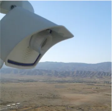
The shadow camera system consists of six cameras taking pic-tures of the ground from the top of an 87 m high solar tower. Together, the pictures cover a 360°view around the tower. If shad-ows fall on the ground, they are seen in the images. The cameras are off-the-shelf standard surveillance cameras (Mobotix MX-M24M-Sec-D22, CMOS sensor) providing 8 bit RGB images with 20481536 pixels every 15 s. The system was established in 2014, upgraded in 2015 and is running during daytimes since then. Two major downtimes were caused by lightning strikes, against which external overvoltage protection is now applied. The expo-sure times of all cameras are set to be constant and equal. All auto-matic adjustments within the cameras have been disabled. One shadow camera is depicted inFig. 1.
The system is situated on the Plataforma Solar de Almería (PSA) in the Tabernas Desert in the south of Spain. Scientists from CIE-MAT (Centro de Investigaciones Energéticas, Medioambientales y Tecnológicas) and DLR (German Aerospace Center) operate several meteorological measurement stations including all-sky imagers, pyranometers, pyrheliometers and the shadow camera system.
In addition to the cameras, the shadow camera system can have access to data from a grid of 20 Si-pyranometer (Apogee SP Series, LICOR LI200 SL and Kipp & Zonen Splite; GHI measurements) described inSchenk et al. (2015), three tracked pyrheliometers (Kipp & Zonen CHP1; DNI measurements) and three shadowball-shaded pyranometers (Kipp & Zonen CMP21; diffuse horizontal irradiance (DHI) measurements). All data aquisition systems are synchronized via an NTP server.
3. Methodology for the creation of irradiance maps
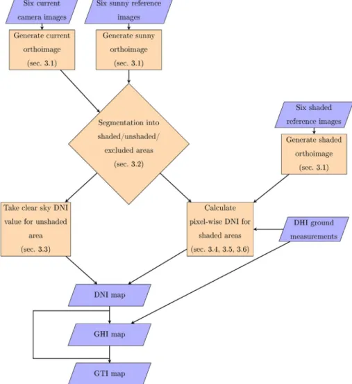
In this section, the methodology to derive spatially resolved irradiance maps is presented in detail. In Section3.1, the process of getting highly spatially resolved images of a test area is explained. Section3.2 presents the methodology to segment the orthoimage into shaded and unshaded areas. For unshaded areas, clear sky irradiance values are taken (see Section3.3). All following sections focus on the measurements of irradiance values in shaded areas: Section3.4introduces basic concepts of image acquisition. The simplified bidirectional reflectance function applicable for our purposes is illustrated in Section3.5. The calculation of the spatially resolved irradiance map itself is explained in Section3.6. A simplification, which does not require additional ground mea-surements, is derived in Section3.7. The flowchart inFig. 2 sum-marizes the approach.
3.1. Generating orthoimages
The shadow cameras described in Section2provide six images every 15 s. The interior orientation of the cameras is determined using methods described inScaramuzza et al. (2006). The external orientation is found using GPS reference coordinates of objects vis-ible in the images. With both the external and the interior orienta-tion known and considering a ground model, these six images are combined to one so-called orthoimage. An example of an orthoim-age is given inFig. 3(left). Orthoimages cover an area of 4 km2 (2 km2 km).
Besides the orthoimage for the timestamp under evaluation (current orthoimage), the shadow camera system uses two refer-ence orthoimages. One referrefer-ence orthoimage (sunny reference) cor-responds to a time when no shadow fell on the PSA (seeFig. 4). The other reference orthoimage (shaded reference) was taken when the PSA was completely shaded. The times of the reference images were determined by all-sky imagers. For a sunny reference times-tamp, no cloud is allowed to be present within 45°around the sun and the general cloud coverage must be below 3%. This ensures that no shadow lies on the area. For the shaded reference times-tamp, the cloud coverage must be above 95% with clouds directly blocking the sun. Unfortunately, this does not completely ensure that the whole area of 4km2is shaded as there could be gaps in the clouds not visible from the positions of the all-sky imagers. Through these gaps, distant areas could be found to be unshaded. In order to follow our approach, we accept this minor uncertainty. As the bidirectional reflectance (see Section3.5for details) of the ground depends on the solar position, the reference images are selected to be taken during the similar solar azimuth and ele-vation angles. For the sunny reference images, the tolerated devia-tions are 3°for both azimuth and elevation angles. For the shaded reference images, the tolerance is 10°. If no reference images are
available, the current timestamp is excluded. This way, the pixel-wise view factors regarding the DNI are relatively constant for the three orthoimages. For the DHI view factors, we must assume Lambertian reflectance. This assumption is further discussed and specified in Section3.6. For all three orthoimages, irradiance mea-surements must be available. The reference orthoimages are allowed to be taken up to 60 days prior to the evaluated timestamp.
The pixels of specular reflective objects are excluded in the orthoimages (see green pixels inFig. 3, right). On the PSA, many metal structures and mirrors are present. If reflections of such an object hit a camera, the pixels corresponding to this area are not evaluable. To exclude these areas, several approaches are applied: Larger structures are ruled out based on their GPS coordinates, which is done in the composition of the orthoimage (see black pix-els inFig. 3, left).
Additionally, reflections present in the current and in the sunny orthoimage are excluded individually for each timestamp based on an empirically found threshold of 60% of the normalized gray images (see green pixels in the north ofFig. 3, right). Also, reflec-tions in the shaded orthoimage are removed via a dynamic thresh-old based on the average and the distribution of the pixel intensities. Shadows of non-cloud objects in the current orthoim-age are detected as they are also present in the sunny reference orthoimage, and are thus ruled out by applying a threshold of 0.05 to the normalized sunny reference orthoimage.
3.2. Segmentation of orthoimages
A pixel in the current orthoimage can either be shaded, unshaded or excluded from validation. The irradiance values for unshaded pixels are not measured by the cameras, but taken from a clear sky irradiance model (see Section3.3). In order to distin-guish between shaded and unshaded areas, the current orthoimage is segmented. This segmentation is explained in this section. The methodology to derive irradiance values for the shaded areas is described in Sections3.4–3.7.
In order to achieve a segmentation of the current orthoimage into shaded and unshaded areas, a difference image is calculated with Eq. (1).S0sunny is the sunny reference linearized orthoimage, S0current is the current linearized orthoimage. To allow thresholds
independent of irradiance levels, the gray images are calculated and normalized by a normalization factor (explanations given in Section3.4).
Diff:imageSunny2Current¼S0sunnyS0current ð1Þ
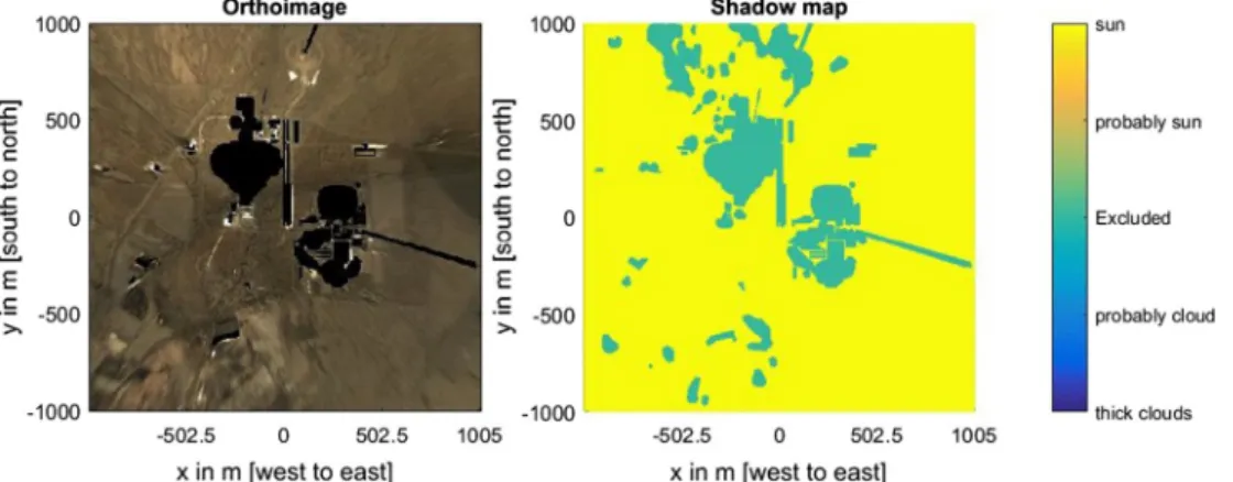
Negative values do not provide information and are set to zero. The thresholds are chosen after visual testing. Empirically, a value of 0.14 was found below which the areas are considered to be unshaded. The areas above this threshold may still obtain clear sky irradiance values, but these are explicitly calculated as explained in the following sections. Other possible segmentation approaches based on the shaded orthoimage are found to be prone to errors. An example of an orthoimage and the corresponding sha-dow map is depicted inFig. 3. As can be seen inFig. 9, optically thin clouds pose a challenge for this segmentation. As the irradiance within a shadow of an optically thin cloud is however close to the clear sky irradiance values (see Fig. 9), the found deviations are small.
3.3. Clear sky irradiance model
The clear sky irradiance model is used to predict both DNI and GHI values as if there were no clouds present. It is derived using the Linke turbidity calculated from ground measurements of the
DNI. Firstly, the Linke turbidity is calculated for all DNI measure-ments in the last 24 h using the Linke turbidity model from Ineichen and Perez (2002). Then cloudy data points are sorted out using the temporal variation of the Linke turbidity as explained inHanrieder et al. (2016) and Wilbert et al. (2016a). Afterwards,
the current Linke turbidity is determined using a time-weighted average of the N most recent Linke turbidities for cloud-free DNI measurements. Together with the airmass of future timestamps this Linke turbidity is used to derive the clear sky irradiances of GHI and DNI based onIneichen and Perez (2002). This approach Fig. 2.Flowchart of the inputs and calculations required to derive irradiance maps.
Fig. 3.PSA on 2015-10-15, 12:48:00 h (UTC + 1). On the left the orthoimage: Shadows are present in the south and east of the considered area. Buildings are excluded (black pixels). The red Xs mark the DNI and DHI stations used for validation in Sections4.2 and 4.3. The small blue circles mark the positions of 20 Si-pyranometer used for validation in Section4.3. Right: Corresponding segmented shadow map, see Section3.2for more details. More pixels are excluded (green) e.g. due to detected reflections. The excluded areas are later interpolated to the nearest non-excluded values. (For interpretation of the references to colour in this figure legend, the reader is referred to the web version of this article.)
is found to be feasible although stationary optically thin clouds can be confused with high Linke turbidities.
3.4. From pixel values to irradiances
The used shadow camera system is based on standard surveil-lance cameras. For such end-user oriented devices, several mathe-matical operations are conducted between the CMOS sensor pixel signals and the resulting image (Poynton, 2003a, p. 203). To derive irradiance values, these operations must be partially reversed.
A spectral irradiance Ekfalling on a pixel’s surface dAduring the
exposure timetexp creates the raw signals of the CMOS sensor’s
pixel. The three signals corresponding to the three color filters are weighted with the camera- and color-dependent spectral responsivity written as
!mn and also weighted with acamera-specific 33 matrix Mcam. Afterwards, the gamma correction
CsRGB is applied. The gamma correction is a nonlinear operation
adjusting the physical photonic measurements to human percep-tion and the sRGB color space. Depending on the camera and its settings, an offset (offset!) must be added. The value of a pixel in the end-user image is thus defined by Eq.(2)(detailed derivation inWilbert (2009)). SsRGB;mn ! ¼
C
sRGB Mcam Z Amn Z kmax kmin texpmn! EkdkdAþoffset! ! ð2ÞIn Eq.(2),S!sRGB;mnrepresents pixelmnof the RGB imageSsRGBwith
its three color channels.kmin;kmaxare the minimum and maximum
wavelengths of the broadband spectrum.Amnis the area of pixelmn.
Ekdenotes the irradiance with wavelengthskdkon sensor areadA
before entering the camera.texpis the exposure time of the camera,
which is constant.
To serve our purposes, the gamma correction is undone. Further-more, each pixel is normalized into the interval [0,1] and converted to grayscale. For the grayscale conversion, the color channels are normalized as described inPoynton (2003b, p. 268). The weighting factorb!Planckfor each color channel is calculated from Planck’s law
and the chosen white balance temperature (10000 K) of the cameras to bebPlanck!¼ ð0:3961;0:3121;0:2918Þ. Thus, the weighting of the
camera-specific matrix Mcamcan be reversed. The offset term was
photometrically measured for one camera and found to be neglect-able. Eq.(2)is thus transformed to Eq.(3):
S0mn¼bPlanck !Z Amn Z kmax kmin texp
mn! EkdkdA ð3ÞThree further assumptions are made: Firstly, the distribution of the spectral irradiance Ek is assumed to be spatially homogeneous for
the area of each singular pixel. Thus, the integral over the pixel area Amn is replaced by a constant. Secondly,
!mn can be different forevery pixel but is assumed to be constant over the area of a given pixel (dA) and the considered wavelength spectrum. Thirdly, the broadband irradiance is defined as the weighted integral of Ekfrom
280 nm to 4000 nm as specified inGueymard and Vignola (1998). With these assumptions, for the pixels with the gamma correc-tion undone, there is a pixel-wise linear relacorrec-tion between the broadband (BB) irradiance EBB;mnand the value of pixelmnin the
linearized grey imageS0 (compare with Grossberg et al. (2003)). constmnwill be found to cancel out for our purposes.
S0mn¼constmnEBB;mn ð4Þ
3.5. Influence of bidirectional reflectance
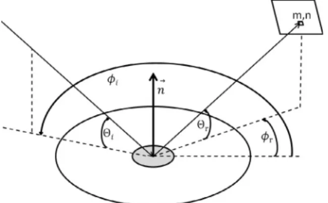
Surfaces look differently if seen under different viewing and illumination geometries. The bidirectional reflectance distribution function (BRDF) describes this effect (Nicodemus, 1965): The value of the BRDF is the angle, surface and wavelength dependent ratio of the radiance seen from a surface element divided by the incident irradiance of this surface (Girolamo, 2003). If the wavelength dependency of the BRDF is to be considered, solar spectra must be measured and must be available to the shadow camera system. The latter is currently not the case. As we thus drop the wavelength dependency, the BRDF is defined for every area projected on the camera pixels and given by Eq.(5). A visualization is depicted in Fig. 5.
BRDFmnðhi;/i;hr;/rÞ ¼
Eout;mnðhr;/rÞ
Ein;mnðhi;/iÞ
constEL;mn ð5Þ
In Eq.(5), Eoutrepresents the reflected or scattered radiance from a
surface area towards a certain direction, Ein is the incident
irradi-ance on the area,hiis the incident elevation angle,/iis the incident azimuth angle,hr is the reflected elevation angle, /r denotes the reflected azimuth angle andconstEL;mnis a pixel-wise constant
mak-ing the BRDF used for our purposes unitless. For all considerations in this section, we look at one arbitrary but specific current times-tamp with corresponding reference timestimes-tamps. As the reference images are chosen to have approximately the same illumination geometry and the viewing geometry is always pixel-wise constant, the angle variables of the BRDFs are omitted. This way, the com-plexity of the BRDF can be reduced significantly.
With Eq.(5)and the properties depicted inFig. 6, the broadband irradiance on a camera sensor pixel EBB;mnis given by Eq.(6).
Fig. 4.PSA on 2015-10-13, 12:48:30 h (UTC + 1). Sunny reference image used to segment the orthoimage displayed inFig. 3. A dark spot in the south-western corner does not correspond to a cloud shadow, which is correctly detected. The timestamps of sunny reference orthoimages are determined via all-sky imagers.
EBB;mn¼
a
mn DNImnBRDFDNI;mnþ XN i¼1 DHImn;iBRDFDHI;mn;i ! ð6Þa
mnis a pixel-wise attenuation factor caused by the camera optics,which also includesconstEL;mn.
a
mnwill be found to cancel out. In Eq.(6), we distinguish between BRDFDNI;mnand BRDFDHI;mn;i. BRDFDNI;mn
is the BRDF for the direction of the direct solar radiation and the viewing geometry. For DNI and one considered timestamp, there is one viewing geometry and one illumination geometry (angle dependency in Eq. (5)). BRDFDHI;mn;i describes the bidirectional
reflectance caused by DHI irradiance coming from the directions of sky segmenti. For DHI, there areNillumination geometries, cor-responding to sky segments. From these sky segments, diffuse radiation reaches the ground and is partially scattered or reflected on camera sensor pixelmn.Fig. 6visualizes Eq.(6).
3.6. Calculation of irradiance maps
As stated before, there are three orthoimages for every times-tamp: The current orthoimage to be evaluated, the sunny reference orthoimage and the shaded reference orthoimage. The reference orthoimages were obtained for approximately the same solar
posi-tion as the image under evaluaposi-tion. We assume that the ground properties did not change significantly between the acquisition times of all three images. This is ensured by limiting the maximum period of time between the orthoimages’ timestamps. The inten-sity independent BRDF is thus the same for the three orthoimages. For all pixels in all orthoimages, Eq.(6)is valid.
However, for the shaded reference orthoimage, the DNI is assumed to be negligible. Thus Eq.(6)can simplified to Eq.(7).
EBB;mn;shaded¼
a
mnXN i¼1
DHImn;i;shadedBRDFDHI;mn;i
!
ð7Þ
We assume that theNsky segments illuminating the area imaged by pixelmncontribute the same to DHIshaded;mn. The single sky
seg-ments can be chosen to fulfill this assumption exactly. In this case, Eq.(7)can be rewritten to Eq.(8).
EBB;mn;shaded¼
a
mnXN i¼1
DHImn;i;shadedBRDFDHI;mn;i
! ¼
a
mnDHIshaded;mn 1 N XN i¼1 BRDFDHI;mn;i ð8ÞFrom Eq.(8), Eq.(9)is derived.
1 N XN i¼1 BRDFDHI;mn;i¼BRDFDHI;mn¼ EBB;mn;shaded
a
mnDHIshaded;mn ð 9ÞConsidering the sunny reference orthoimage, we adapt Eq.(6)to get Eq.(10).
EBB;mn;sunny¼
a
mn DNImn;sunnyBRDFDNI;mnþXN i¼1
DHImn;i;sunnyBRDFDHI;mn;i
!
ð10Þ As for the shaded reference orthoimage, we assume that theNsky segments contribute homogeneously to the DHI of the area imaged by pixelmn. In order to use Eq.(9)for Eq.(10), theNsky segments of the sunny and shaded orthoimage must be the same. Thus, we assume that the angular diffuse radiance distribution over theN sky segments is the same as for the shaded reference orthoimage. This is an approximation. The deviations from this approximation are usually limited as the DHImn;sunny (e.g. 100 W/m2) and
DHIshaded;mn(e.g. 200 W/m2) values are often rather small in
compar-ison to DNImn;sunny(up to 1200 W/m2or more). This is, however, not
always the case. We have to accept this assumption in order to pro-ceed to Eq.(11):
EBB;mn;sunny¼
a
mn DNImn;sunnyBRDFDNI;mnþXN i¼1
DHImn;i;sunnyBRDFDHI;mn;i
!
¼
a
mn DNImn;sunnyBRDFDNIþDHImn;sunnyBRDFDHI;mn
¼
a
mn DNImn;sunnyBRDFDNI;mnþDHImn;sunnyEBB;mn;shaded
a
mnDHImn;shaded
ð11Þ Eq.(11)is used to determine BRDFDNI;mn;sunny¼BRDFDNI;mn:
BRDFDNI;mn¼
EBB;mn;sunnyEBB;mn;shadedDHIDHImn;sunny
mn;shaded
a
mnDNImn;sunny ð12Þ
With both BRDFs determined, we apply Eq. (6) on the current orthoimage:
EBB;mn;current¼
a
mn DNImn;currentBRDFDNI;mnþXN i¼1
DHImn;i;currentBRDFDHI;mn;i
! ð13Þ As for the shaded and sunny orthoimage, we assume that theNsky segments contribute homogeneously to the DHI of the area imaged Fig. 5.The bidirectional reflectance depends on both viewing and illumination
geometry. The illumination geometry is defined by the azimuth angle/iand the
elevation anglehi. The viewing geometry is defined by the azimuth angle/rand the
elevation anglehr.~nis the surface normal,mnis a camera sensor pixel.
Fig. 6.Visualization of Eq.(6): The area seen in pixelmnis illuminated both directly from the sun (solid line, described by BRDFDNI;mnDNImn) and indirectly via light scattering clouds (i¼jandi¼k) and Rayleigh scattering (i¼r), pictured by the dotted lines and described by BRDFDHI;mn;iDHImn;i.
by pixelmn. Thus, we assume that the angular diffuse radiance dis-tribution over theNsky segments is the same for all three orthoim-ages. For the current orthoimage, depending on the situation, this is generally not a close approximation. However, for situations rele-vant for benchmarking all-sky imager based nowcasting systems with cloud coverages below 80%, the deviations caused by this assumption are limited by the usually rather small DHImn;current
val-ues in comparison to DNImn;current. We accept this simplification in
order to proceed. Note that this assumption could be overcome by using additional sensors, which resolve the angular radiation distributions.
EBB;mn;current¼
a
mn DNImn;currentBRDFDNI;mnþDHImn;currentBRDFDHI;mn¼
a
mn DNImn;current EBB;mn;sunnyEBB;mn;shaded DHImn;sunny DHImn;shadeda
mnDNImn;sunny 0 @ þDHImn;current EBB;mn;shadeda
mnDHImn;shaded ð14Þ From Eq.(14), we obtain the desired DNI for the area shown by pixelmn(Eq.(15)). The pixel-wise attenuation constant of the cam-era opticsa
mncancels out.DNImn;current¼
EBB;mn;currentEBB;mn;shadedDHIDHImn;currentmn;shaded
EBB;mn;sunnyEBB;mn;shaded DHImn;sunny
DHImn;shaded
DNImn;sunny
ð15Þ
If Eq.(4)is inserted into Eq.(15), the pixel-wise constant factor constmncancels out as it is the same for every orthoimage.constmn
is the same for every orthoimage since it is determined by camera properties, which are set to be fixed. For this assumption, the con-stants are allowed to be different between every pixel of each of the six shadow cameras utilized. The DNI in Eq.(15)is thus written as: DNImn;current¼ S0mn;currentS0mn;shaded DHImn;current DHImn;shaded S0mn;sunnyS0mn;shaded DHImn;sunny DHImn;shaded DNImn;sunny ð16Þ
S0mn;jare the linearized images described in Section3.4. To calculate spatially resolved DNI maps for all pixelsmn, the three orthoimages S0mn;j, clear sky DNI data for the time of the sunny reference
orthoim-age and three DHI maps are needed. For the sunny reference, the ground measurements DNImn;sunny and DHImn;sunny can safely
assumed to be constant over the whole imaged area. For the shaded reference, we also assumed DNImn;shadedto be zero for all pixels (Eq.
(8)). In general, DHImn;shadedand DHImn;currentare not homogeneous
over the whole imaged area, especially for scattered clouds during the timestamp under evaluation. As no spatially resolved DHI mea-surements are available, the DHI is measured and assumed to be the same for all pixels. This assumption, especially for the specific situations of the current orthoimage, results in deviations (see Section4.5). For most cases, these deviations are small in compar-ison to the DNI. With these approximations, we can derive the DNI in the shaded areas imaged in camera pixelmn to be given by Eq.(17): DNImn;current¼ S0mn;currentS0mn;shaded DHIcurrent DHIshaded S0mn;sunnyS0mn;shaded DHIsunny DHIshaded DNIsunny ð17Þ
Assuming a spatially homogeneous DHI, GHI maps can be derived with Eq.(18), where
a
s is the sun elevation angle. GHI and DNIcan then be used to derive GTI, using the Skartveit-Olseth method (Skartveit and Olseth, 1986), which was found to be most accurate for the PSA (Demain et al., 2013; Noorian et al., 2008; Kambezidis et al., 1994).
GHImn¼DNImnsinð
a
sÞ þDHI ð18ÞThe irradiance data obtained this way for the shaded areas is then combined with the irradiance value for the unshaded areas (see Section3.3). The images are cleaned by morphological operations, which remove unrealistically small shadows, define minimum irra-diance values (0 W/m2) and maximum irradiance values (clear sky irradiance). Previously excluded pixels are interpolated. This way, spatially resolved reference irradiance maps are generated. 3.7. Further simplification: omitting ground measurements
For Eq.(17), DNIsunny can be retrieved from clear sky models. If
we further (pixel-wise) assume that DHIshaded¼DHIcurrent¼
DHIsunny, Eq. (17) can be transformed to Eq.(19). This way, no
ground measurements besides the cameras are needed to derive irradiance maps.
DNImn;current¼
S0mn;currentS0mn;shaded
S0mn;sunnyS0mn;shaded
DNIsunny ð19Þ
Although the assumption leading to Eq. (19) adds errors, these errors are limited asS0mn;shaded, the shaded reference orthoimage, is much smaller than S0mn;sunny and allS0mn;current with significant DNI. The deviations caused by the assumption are investigated in the validation (see Section4). The linear relation between the current linearized image and the pixel-wise DNI is illustrated inFig. 7.
4. Validation of the shadow camera system
In this section, the validation of the shadow camera system is presented. Firstly, a visual and qualitative comparison between orthoimages and irradiance maps is performed in Section4.1. In the second step, calculated DNI (Section4.2) and GHI (Section4.3) maps are validated against ground measurements with 911 one-minute averages on two days and analyzed in detail. The two example days are chosen to be relevant for nowcasting applica-tions and have different cloud coverages and variabilities. In Sec-tion4.4, the validation results for three further days are briefly presented. A summary is given in Section4.5.
The validation of both DNI and GHI maps is conducted for one-minute averages. These one-one-minute averages are the pixel-wise mean values of 5 irradiance maps at 0, 15, 30, 45 and 60 s for each minute. If not all irradiance maps could be calculated, the minute is excluded from the validation. The one-minute averages of the irra-diance maps are compared against ground measurements, which are also averaged to full minutes. To validate the DNI and GHI maps, 3 and 23 ground stations are used, respectively. The irradi-ances at the pixels containing the radiometers are compared to
Fig. 7.Visualization of Eqs.(17) and (19). With the gamma correction undone and all assumptions applied, we find a linear relation between the pixel-wise DNI of the timestamp under evaluation and the corresponding, modified camera output.
the corresponding ground measurements. For one station, these comparisons are shown inFigs. 8, 10, 12 and 13.Figs. 9 and 11 depict close-ups ofFigs. 8 and 10. As spatial averages are of special interest, we also compare the average irradiance of the pixels con-taining a radiometer to the average of all radiometer readings for every timestamp.
4.1. Visual validation
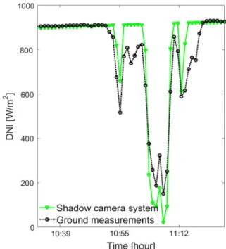
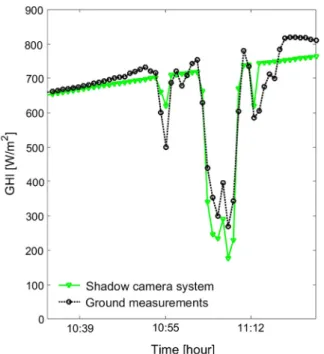
Looking atFig. 9, 10:55 h, we see that some thin clouds are not detected as their shadows’ brightnesses are above the chosen threshold. The clear sky DNI model shows only small deviations from the ground measurements.Fig. 10depicts the GHI on 2015-09-18. The clear sky GHI model shows deviations in the presence of clouds (seeFig. 11). This is caused by DHI and is discussed in Section4.3. The DNI on the 2015-09-19 is depicted inFig. 12. We see small deviations between the shadow camera system and the ground measurements. InFig. 13, the GHI for this day is shown. Especially between 11:00 h and 13:00 h, overshootings of the GHI beyond the clear sky GHI level are observed. This behavior is caused by DHI and is discussed in Section 4.5. In general, there are only small deviations visible between the values derived from the shadow camera system and the ground measurements.
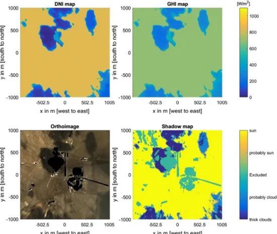
Every 15 s, the four images depicted inFig. 14are available: The orthoimage, the shadow map, and irradiance maps (here: DNI and GHI, GTI is also possible). Visual validations found a well-working shadow segmentation algorithm for sun elevation angles above 10°. For smaller elevations, the sun shines directly into at least one camera, causing reflections and saturations. This problem was solved by an aperture attached to the cameras in December 2016. Thus, the validation presented here is restricted to elevation angles above approximately 10°. Independent from the irradiance measurements, which are validated in the next two sections, the capacity to detect shadows on the ground itself is highly useful for benchmarking all-sky imager based nowcasting systems or for providing warnings to large solar power plants.
4.2. Quantitative validation of DNI maps
In this section, DNI maps for two example days are validated in detail. The DNI maps are calculated using DNI and DHI ground measurements as explained in Section3.6and Eq.(17). Moreover,
DNI maps calculated via the simplified method presented in Sec-tion3.7and Eq.(19) are validated. The simplified method does not require additional ground measurements besides the shadow camera images.
The errors for the DHI-based method (Eq.(17)) are given both in absolute and relative figures inTable 1. The errors for the simpli-fied method, not requiring additional ground measurements (Eq. (19)), are presented inTable 2. Three stations depicted inFig. 3 (red Xs) are used to validate the DNI maps. Station 1 is the south-ernmost station inFig. 3, station 2 the easternmost and station 3 the northernmost. The clear sky irradiance model (see Section3.3) is based on station 1 but the corresponding irradiance maps’ pixel is not specially treated with e.g. normalizations. Therefore, station 1 is included in the validation.Mean DNIis the daily mean DNI as Fig. 8.Comparison of DNI values measured by station 1 (southernmost inFig. 3) on
2015-09-18 to the corresponding pixel in the DNI maps derived from the shadow camera system. On this day, very few clouds were present.
Fig. 9.Close-up ofFig. 8: Deviations exist for optically thin clouds at 10:55 h and 11:12 h. The shading of the optically thick cloud present around 11:05 h is determined with high accuracy in time and irradiance.
Fig. 10.Comparison of GHI values measured by station 1 (southernmost inFig. 3) on 2015-09-18 to the corresponding pixel in the GHI maps derived from the shadow camera system.
measured by the ground stations for the validation timestampsTd.
The same dataset in one-minute resolution as for the visual valida-tion in Secvalida-tion4.1is taken. The spatial average (Spatial avg) depicts the deviation of the ground measurements to the corresponding pixels of the shadow camera system averaged for every considered minute among the three stations and pixels. It is the deviation of the average rather than the average of the deviations. The formulas for root mean squared errors (RMSE), mean absolute error (MAE), standard deviation (std) and bias are given in Eqs.(20)–(23). Td
equals the number of one-minute averages per day with Td¼396 for 2015-09-18 andTd¼515 for 2015-09-19,pidenotes
the values predicted by the shadow camera system for the pixel corresponding to a specific station and oi is the corresponding
ground measurements. Relative deviations are calculated via the daily mean irradiance as measured by the radiometer.
RMSE¼ ffiffiffiffiffiffiffiffiffiffiffiffiffiffiffiffiffiffiffiffiffiffiffiffiffiffiffiffiffiffiffiffiffiffiffiffiffiffiffiffiffi 1 Td XTd i¼1ðpioiÞ 2 s ð20Þ MAE¼ 1 Td X Td i¼1 jpioij ð21Þ STD¼ ffiffiffiffiffiffiffiffiffiffiffiffiffiffiffiffiffiffiffiffiffiffiffiffiffiffiffiffiffiffiffiffiffiffiffiffiffiffiffiffiffiffiffiffiffiffiffiffiffiffiffiffiffiffiffiffiffiffiffiffiffiffiffiffiffiffiffiffiffiffiffiffiffiffiffiffiffiffiffiffiffiffiffiffiffiffiffiffiffiffiffiffiffiffiffi 1 Td1 XTd i¼1 ðpioiÞ 1 Td XTd j¼1ðpjojÞ 2 s ð22Þ BIAS¼ 1 Td X Td i¼1 pioi ð23Þ
InTable 1, the DNI maps calculated with Eq.(17)are validated. For 2015-09-18 and the three pyrheliometers, the deviations are small: Relative RMSE are between 4.2% and 7.0%, relative MAE are between 1.6% and 2.0%, relative standard deviations are between 4.2% and 6.8% and the biases are negligible. On this partic-ular day, there were very few clouds present (seeFigs. 8 and 10). The shadow camera system correctly detects the unshaded areas and applies the clear sky DNI as explained in Section 3.2. For 2015-09-19, the deviations are larger: relative RMSE between 13.6% and 16.7%, relative MAE between 4.8% and 7.5% and standard deviations between 10.1% and 15.4%. Again, the bias is small. The spatial average (spatial avg) for both days is often smaller than the stations’ deviations, but not significantly smaller. In the follow-ing, sources of these deviations are discussed.
In general, the segmentation between shaded and unshaded areas works well. However, for optically thin clouds, the shadows are too bright for the chosen segmentation thresholds. Careful examinations ofFigs. 8 and 12show that this source of errors only plays a minor role. In Table 1, the deviations for station 3 are always the largest. This is due to the specific location of this sta-tion: Placed on top of a building, whose corresponding pixels in the orthoimages are excluded (see Section3.1), the irradiance val-ues for the pixel corresponding to the location of station 3 are only interpolated and not derived from Eq.(17). This adds errors for two reasons. First of all, the interpolation itself is less accurate than the actual evaluation of the pixel with Eq.(17). Moreover, station 3 is placed on a building approximately 10 m above the ground which is not considered in the interpolation. Although a large area around station 3 must be interpolated due to buildings and mirrors, the deviations are not significantly larger than for the other stations. Fig. 11.Close-up ofFig. 10: The deviations are in general smaller in comparison to
Fig. 9. However, DHI overshootings present around 11:15 h are not detected.
Fig. 12.Comparison of DNI values measured by station 1 (southernmost inFig. 3) on 2015-09-19 to the corresponding pixel in the DNI maps derived from the shadow camera system. On this day, many transient clouds were present.
Fig. 13.Comparison of GHI values measured by station 1 (southernmost inFig. 3) on 2015-09-19 to the corresponding pixel in the GHI maps derived from the shadow camera system. Due to light scattering on clouds, DHI overshootings are visible.
Fig. 14.Orthoimage, shadow map, DNI and GHI maps for an example timestamp (2015-09-19, 11:02:00 h UTC + 1). From the orthoimage and a reference orthoimage, the segmentation into shaded and unshaded areas is derived (shadow map). Different approaches for these two areas lead to irradiance maps (here: DNI and GHI, GTI is also possible). The colorbar for the GHI and the DNI map is the same. (For interpretation of the references to colour in this figure legend, the reader is referred to the web version of this article.)
Table 1
Validation of DNI maps calculated with Eq.(17)using DHI ground measurements.Spatial avgis the deviation of the ground measurements to the corresponding pixels of the shadow camera system averaged for every considered minute among the three stations and pixels, and not the average of the daily deviations calculated for each station: the deviation of the average rather than the average of the deviation.
Eq.(17) Station Mean DNI RMSE MAE STD BIAS
(s.Fig. 3) W/m2 W/m2 % W/m2 % W/m2 % W/m2 % 2015-09-18 Station 1 871.7 44.5 5.1 13.6 1.6 43.8 5.0 8.3 0.9 Station 2 876.0 36.5 4.2 13.9 1.6 36.5 4.2 1.1 0.1 Station 3 873.2 61.0 7.0 17.8 2.0 59.6 6.8 13.1 1.5 Spatial avg 873.6 37.3 4.3 11.8 1.4 36.5 4.2 7.5 0.9 2015-09-19 Station 1 660.6 89.6 13.6 42.9 6.5 82.5 12.5 35.2 5.3 Station 2 683.8 72.3 10.6 32.9 4.8 69.3 10.1 20.9 3.1 Station 3 713.3 119.4 16.7 53.7 7.5 110.1 15.4 46.4 6.5 Spatial avg 685.9 68.7 10.0 38.8 5.7 59.7 8.7 34.2 5.0 Table 2
Validation of DNI maps calculated with the simplified Eq.(19), which does not require DHI ground measurements.Spatial avgis the deviation of the ground measurements to the corresponding pixels of the shadow camera system averaged for every considered minute among the three stations and pixels, not the average of the deviations calculated for each station.
Eq.(19) Station Mean DNI RMSE MAE STD BIAS
(s.Fig. 3) W/m2 W/m2 % W/m2 % W/m2 % W/m2 % 2015-09-18 Station 1 871.7 58.0 6.7 16.3 1.9 57.3 6.6 9.3 1.1 Station 2 876.0 48.1 5.5 15.9 1.8 48.1 5.5 1.3 0.1 Station 3 873.2 45.8 5.2 14.4 1.7 45.1 5.2 8.1 0.9 Spatial avg 873.6 47.0 5.4 14.7 1.7 46.6 5.3 6.2 0.7 2015-09-19 Station 1 660.6 141.6 21.4 57.1 8.6 132.4 20.0 50.6 7.7 Station 2 683.8 83.4 12.2 35.2 5.2 80.3 11.8 22.6 3.3 Station 3 713.3 90.1 12.6 42.4 5.9 84.2 11.8 32.4 4.5 Spatial avg 685.9 80.4 11.7 40.5 5.9 72.4 10.6 35.2 5.1
This demonstrates the robustness of the chosen approach and its feasibility for real scenarios with obstacles present. One major source of errors results from the hardware itself: As standard surveillance cameras are utilized, the accuracy and consistency of exposure time and sensitivity is unknown. Moreover, deviations result from the approximations made to derive Eq.(17). The clear sky DNI used for the unshaded areas is validated to be accurate for the evaluation time of the shadow camera system.
In conclusion, the validation of the shadow camera system based on Eq.(17)demonstrates its applicability to derive spatially resolved DNI maps. The spatial averages (spatial avg), although only averaged over three pixels, hint at the spatial aggregation effects effective for field averages: As explained in Section1and inKuhn et al. (2017b)as well asKuhn et al. (2017a), the behavior of aggregated field averages is different from point measurements. As field averages are more relevant for industrial applications, point measurements and derived comparisons against persistence forecasts must be treated with care.
InTable 2, DNI maps calculated with Eq.(19)are validated. This method does not require ground measurements besides the sha-dow cameras as the clear sky DNI can be derived from models. The deviations of such a system without irradiance ground mea-surements strongly depend on the validity of the spatially constant DHI assumption among the timestamps of the orthoimages and on the clear sky DNI model used, derived for instance from NWP data. For the validation presented inTable 2, the same clear sky predic-tion as for the validapredic-tion presented inTable 1is used.Table 2is thus a validation of the further assumptions made in Section3.7 to derive Eq.(19). Comparing the spatial averages inTables 1 and 2, a minor increase in the deviations is present. The deviations of the stations depict a heterogeneous behavior: The errors for station 3 are smaller for the simplified method. As mentioned, the pixel corresponding to station 3 cannot be measured directly and is only interpolated. Although the same interpolation method is applied in both cases, these results must be treated with care. Station 2 depicts larger deviations if the simplified method is applied and this simplified method results in far larger deviations for station 1. Detailed analysis show that these significantly higher deviations for station 1 mainly result from transient clouds between 11:00 h and 13:00 h, when the DHI indeed played a major role (visible in the overshootings inFig. 13). As the RMSE gives a high weight to large errors, the lack of DHI information in Eq.(19)results in far larger deviations in comparison to Eq. (17). For field averages, these deviations tend to be smaller due to aggregation effects, at which the deviations for the spatial average (Spatial avg) again hint.
In general, the deviations of the simplified method are still suf-ficiently small for the purposes of this shadow camera system. However, they strongly depend on the utilized method to derive the clear sky DNI required in Eq.(19).
4.3. Quantitative validation of GHI maps
The validation of GHI maps derived from the shadow camera system is conducted over the same dataset as the validation of the DNI maps in the previous section. For the validation of GHI maps, 23 radiometers (seeFig. 3) are used.Station avgis the aver-age of the daily deviations for each station. The mean GHI averaver-aged for all stations and timestamps is 714.8 W/m2for 2015-09-18 and
599.2 W/m2for 2015-09-19. The deviations are similar amongst
the stations with a standard deviation of the absolute RMSE between the stations of 6.0 W/m2 for 2015-09-18 and 7.5 W/m2
for 2015-09-19. The spatial average (Spatial avg) depicts the devi-ation of the ground measurements to the corresponding pixels of GHI maps calculated by the shadow camera system averaged for
every considered minute among the 23 stations and pixels, taking spatial aggregation effects into account.
InTable 3, GHI maps calculated with Eqs.(17) and (18)are val-idated. All deviations are below 10%. As 23 pixels corresponding to 23 ground stations are averaged in the spatial average, field aggre-gation effects are more visible than in the spatial average ofTable 1, which is calculated from three pixels and stations. InFig. 13, there are many timestamps when the GHI measured by the ground sta-tions exceeds the GHI values derived from the shadow camera sys-tem. These overshootings are the results of clouds reflecting or scattering light at a specific location. These DHI values are spatially very inhomogeneous and hard to predict. Most likely, these over-shootings are the reason for the positive bias found for DNI maps and for the negative biases of the GHI maps. For field averages, these overshootings play a minor role. For CSP applications, DHI values are of minor importance and there is usually an upper power generation limit for PV applications. For these reasons, ignoring the overshootings in further analyses seems acceptable.
Table 4presents the validation of the simplified method (Eq. (19)). To calculate GHI maps without additional ground measure-ments, a DHI model is needed. The deviations of this simplified approach strongly depend on the quality of this DHI model as well as on the chosen clear sky DNI model (see discussion ofTable 2).
For this analysis, the same DHI is used in Eq.(18) for both Tables 3 and 4. Also, the same clear sky DNI is used. The difference between the validation presented inTables 3 and 4is thus only the difference between Eqs.(17) and (19). All in all, Eqs.(17) and (19) yield similar results for GHI maps. This is due to the deviations added by assuming a spatially homogeneous DHI needed for Eq. (18). In general, the deviations found for GHI maps calculated with both methods are small (3.3–0.4%).
4.4. Validation results on further days
Besides the two example days discussed in the previous sec-tions, three further days are validated and briefly discussed. These days are 2016-05-11, 2016-09-01 and 2016-12-12. The irradiance maps for these days are calculated using Eq.(17). 2016-05-11 is a day with many transient clouds (similar to 2015-09-19), which has a mean daily DNI of 790.0 W/m2and a mean GHI of 785.6 W/m2. Its
validation is conducted with two pyrheliometers and 15 pyra-nometers on 425 one-minute averages. 2016-09-01 shows less transient clouds than 2016-05-11 and has a mean daily DNI of 758.3 W/m2and a mean GHI of 733.7 W/m2. Two pyrheliometers
and 19 pyranometers on 393 one-minute averages are included in the validation of this day. 2016-12-09 is an overcast day with a mean daily DNI of 4.0 W/m2 and a mean GHI of 126.8 W/m2.
The validation of this day is done on 510 one-minute averages with two pyrheliometers and 17 pyranometers.
The deviations found for these further days are displayed in Tables 5 and 6. They are similar to the deviations of discussed in the previous sections. Due to the small absolute DNI values on 2016-12-09, the relative properties are large although the absolute values are similar to the values found for 2015-09-18. In total, the shadow camera system is validated on five days with 2239 one-minute averages (37.3 h).
4.5. Summary of results
Considering DNI maps, the deviations found by validations are similar to all-sky imager derived irradiance maps at lead time 0 min and smaller than the deviations found for forecasts (Kuhn et al., 2017a,b). Comparing the deviations of the GHI maps gener-ated by the shadow camera system to satellite-based forecasts with low temporal and spatial resolution is delicate. However, if compared directly, deviations in the order of 12% RMSE (GHI)
(Zelenka et al., 1999) or above (Perez et al., 2015) have been reported for satellite-based methods, which are similar or higher than the deviations found for the shadow camera system. Consid-ering that off-the-shelf, low-cost and photometrically uncalibrated cameras were used, the deviations found in the validations are small. These small deviations are the result of the use of reference images (sunny and shaded reference orthoimage), the well-working segmentation into shaded and unshaded areas and the accurate clear sky DNI model used for the unshaded areas. In sum-mary, the shadow camera system provides DNI and GHI maps at spatial resolutions of 5 m5 m for 2 km2 km. For the two example days studied in detail, the deviations are below 9% RMSE for GHI maps and below 10% RMSE for DNI maps and spatial aver-ages over the available stations (23 for GHI, 3 for DNI). The devia-tions of the three further days evaluated in Section4.4are similar.
With these deviations, the shadow camera system is able to bench-mark all-sky imager derived nowcasts for all lead times.
5. Discussion of differences between all-sky imager based and hypothetical shadow camera based nowcasting systems
Potentially, the principle of the shadow camera system could be used to forecast irradiance maps. Such hypothetical shadow cam-era based nowcasting systems show distinct differences in com-parison to all-sky imager based nowcasting systems:
1. One major challenge for all-sky imager based nowcasting sys-tems is the segmentation of clouds around to the sun. As the pixels of the sun in the images are often oversaturated, the exact shape of small clouds directly in front of the sun is hard Table 3
Validation of GHI maps calculated with Eqs.(17) and (18).Station avgis the average of the daily deviations for each station,Spatial avgis depicts the daily deviations averaged amongst all 23 stations for each timestamp.
Eq.(17) Station RMSE MAE STD BIAS
(s.Fig. 3) W/m2 % W/m2 % W/m2 % W/m2 % 2015-09-18 Station avg 29.7 4.2 19.5 2.7 28.0 3.9 7.1 1.0 Spatial avg 23.4 3.3 15.1 2.1 23.1 3.2 3.7 0.5 2015-09-19 Station avg 57.3 9.6 42.6 7.1 47.4 7.9 30.9 5.1 Spatial avg 52.2 8.7 42.2 7.0 39.3 6.6 34.4 5.7 Table 4
Validation of GHI maps calculated with Eqs.(19) and (18).Station avgis the average of the daily deviations for each station,Spatial avgis depicts the daily deviations averaged amongst all 23 stations for each timestamp. The simplified method does not require DHI ground measurements to calculate DNI maps, but DHI ground measurements are used to calculate the GHI maps. These measurements can be replaced by a DHI model, avoiding the necessity of ground measurements for GHI maps.
Eq.(19) Station RMSE MAE STD BIAS
(s.Fig. 3) W/m2 % W/m2 % W/m2 % W/m2 % 2015-09-18 Station avg 35.2 4.9 20.7 2.9 33.9 4.7 7.2 1.0 Spatial avg 30.7 4.3 17.3 2.4 30.3 4.3 4.7 0.7 2015-09-19 Station avg 62.1 10.4 44.4 7.4 53.7 9.0 29.9 5.0 Spatial avg 48.8 8.2 37.0 6.2 39.6 6.6 28.7 4.8 Table 5
Validation of DNI maps calculated with Eq.(17)for three further days. The deviations are similar to the deviations discussed in Section4.2. Due to the overcast situation present on 2016-12-09, the relative deviations are huge, but the absolute deviations are the smallest found for all five days.
Eq.(17) Station RMSE MAE STD BIAS
(DNI) (s.Fig. 3) W/m2 % W/m2 % W/m2 % W/m2 % 2016-05-11 Station avg 126.5 16.3 53.6 6.9 124.9 16.0 9.7 1.3 Spatial avg 93.4 12.0 49.8 6.4 93.0 12.0 9.7 1.2 2016-09-01 Station avg 79.6 10.5 52.5 7.0 65.7 8.7 44.2 5.9 Spatial avg 69.0 9.1 49.7 6.6 53.1 7.0 44.2 5.9 2016-12-09 Station avg 45.1 1260.1 22.0 608.8 41.7 1167.9 17.2 473.5 Spatial avg 43.2 1200.8 21.9 608.4 39.6 1102.9 17.2 477.4 Table 6
Validation of GHI maps calculated with Eqs.(17) and (18)for three further days. The deviations are similar to the deviations discussed in Section4.3.
Eq.(17) Station RMSE MAE STD BIAS
(GHI) (s.Fig. 3) W/m2 % W/m2 % W/m2 % W/m2 % 2016-05-11 Station avg 98.0 12.1 71.4 8.8 67.7 8.4 68.2 8.4 Spatial avg 89.8 11.1 72.3 8.9 53.5 6.6 72.2 8.9 2016-09-01 Station avg 46.8 6.2 37.4 4.9 32.8 4.3 30.6 4.0 Spatial avg 39.9 5.3 33.5 4.4 25.8 3.4 30.6 4.0 2016-12-09 Station avg 40.1 25.0 32.3 20.2 34.6 22.7 15.8 8.0 Spatial avg 43.7 26.3 33.1 19.9 31.6 19.0 30.5 18.4
to determine. Shadow cameras do not face this challenge as they are taking images of the ground, but mirrors present in CSP plants or PV modules are equally hard to evaluate. 2. For all-sky imager based nowcasting systems, cloud height
determination is a challenge. For low sun elevation angles, this results in relative larger errors in the calculated shadow posi-tions on the ground. A shadow camera system directly detects the shadow on the ground with small deviations.
3. As for cloud heights, the exact determination of cloud shapes is a challenge for all-sky imager based approaches. The shadow camera system directly detects the shadow of the cloud on the ground.
4. In principle, all-sky imager based nowcasting can be operated in every location. Shadow cameras need a relatively flat area under consideration and an elevated position as from their positions the relevant area must be visible. In the absence of close-by mountains, towers (e.g. in solar tower plant) or other man-made elevations (churches, power poles) can be taken advantage of. A low elevation can be compensated by high-resolution cameras, by increasing the amount of cameras or with spatially distributed cameras.
5. An all-sky imager based nowcasting system can detect and track clouds in various heights. As the shadow camera system only sees the shadows on the ground, situations with multiple cloud heights and height-dependent wind directions might be challenging.
6. Maintenance and cleaning tend to be much easier for shadow cameras, as the optics are facing downwards and are thus better protected against dust and birds than all-sky imagers. For the reasons mentioned above, shadow camera systems look like promising short-term forecasting tools for the solar industry.
6. Conclusion and future work
In this publication, a novel, robust and low-cost shadow camera system is presented and validated. The system is capable to mea-sure spatial irradiance distributions over several square kilometers. The generated spatially resolved irradiance maps have been used to validate and improve nowcasting systems. Furthermore, they can support both electrical grid operators and solar power plant operators with irradiance information. To the best of our knowl-edge, this is the first time spatially resolved irradiance maps gener-ated by shadow cameras are reported.
An all-sky imager based nowcasting system validated for the same days as the shadow camera system shows one minute aver-aged RMSE deviations for the current situation (lead time zero) of 7.1 (2015-09-18)–26.2% (2015-09-19) (Blanc et al., 2017; Kuhn et al., 2017a,b), which is above the deviations of 4.2–16.7% RMSE for DNI maps of the shadow camera system. Thus, the shadow camera system seems to be a feasible tool to validate all-sky ima-ger derived nowcasts. Previously, all-sky imaima-ger based nowcasting systems were only validated using a few radiometer stations and compared to persistence forecasts derived from these stations. As aggregated field averages display different behavior than point measurements and are more relevant for industrial applications, spatially resolved irradiance maps as provided by the shadow cam-era system should be used to validate nowcasting systems with special emphasis given to spatial aggregation effects. In the absence of a shadow camera system, the spatial aggregation effects could be estimated by an auto-evaluation of a nowcasting system: This can be achieved by comparing irradiance maps predicted on different timestamps but for the same timestamp (different lead times). However, having an independent reference system is advantageous. Considering spatial averages is important as they
have usually higher accuracies than pixel comparisons are (see Section4).
The presented shadow camera system will be further improved regarding its nowcasting capability, hardware adjustments to cope with low sun elevation angles and optimized DNI and GHI clear sky models. Future work also includes the validation of GTI maps derived from the shadow camera system. The hardware of the sha-dow camera system is further used to validate a cloud speed sensor and to derive cloud heights, which will be presented in future pub-lications. Validations of NWP derived cloud motion vectors with velocities derived from the shadow cameras might also be done in future work. Presumably, the shadow camera system could struggle if installed in locations with generally high Linke turbidi-ties or predominantly optically thin clouds. This will be studied in future work.
In order to master electrical grids with high penetrations of solar power plants and to optimize the operations of large solar plants, forecasting tools are the key factor. The shadow camera sys-tem can help to improve these tools by providing validation refer-ences with high temporal and high spatial resolutions and can potentially act as a nowcasting system itself, having distinct advantages in comparison to all-sky imager based approaches.
Acknowledgements
The research presented in this publication has received funding from the European Union’s Horizon 2020 programme for the initial development of the shadow camera system (PreFlexMS, Grant Agreement No. 654984). With founding from the German Federal Ministry for Economic Affairs and Energy within the WobaS pro-ject, the generation of irradiance maps was implemented. The European Union’s FP7 programme under Grant Agreement No. 608623 (DNICast project) financed operations of all-sky imagers and other ground measurements.
References
Alonso, J., Ternero, A., Batlles, F.J., López, G., Rodríguez, J., Burgaleta, J.I., 2014. Prediction of cloudiness in short time periods using techniques of remote sensing and image processing. Energy Proc. 49, 2280–2289 http:// www.sciencedirect.com/science/article/pii/S187661021400695X.
Andreev, M.S., Chulichkov, A.I., Emilenko, A.S., Medvedev, A.P., Postylyakov, O.V., 2014. Estimation of cloud height using ground-based stereophotography: methods, error analysis and validation. Proc. SPIE 9259. 92590N-92590N-6
http://proceedings.spiedigitallibrary.org/proceeding.aspx?articleid=1974843. Blanc, P., Massip, P., Kazantzidis, A., Tzoumanikas, P., Kuhn, P., Wilbert, S., Schüler,
D., Prahl, C., 2017. Short-term forecasting of high resolution local DNI maps with multiple fish-eye cameras in stereoscopic mode. AIP Conf. Proc. 1850 (1), 140004. http://dx.doi.org/10.1063/1.4984512. http://aip.scitation.org/doi/abs/ 10.1063/1.4984512.
Chow, C.W., Urquhart, B., Lave, M., Dominguez, A., Kleissl, J., Shields, J., Washom, B., 2011. Intra-hour forecasting with a total sky imager at the UC San Diego solar energy testbed. Sol. Energy 85 (11), 2881–2893 http:// www.sciencedirect.com/science/article/pii/S0038092X11002982.
de WA, W., 1885. The heights of clouds. Nature 32, 630–631 http:// www.nature.com/nature/journal/v32/n835/abs/032630b0.html.
Demain, C., JournCée, M., Bertrand, C., 2013. Evaluation of different models to estimate the global solar radiation on inclined surfaces. Renew. Energy 50, 710– 721http://www.sciencedirect.com/science/article/pii/S0960148112004570. Fung, V., Bosch, J.L., Roberts, S.W., Kleissl, J., 2014. Cloud shadow speed sensor.
Atmos. Measure. Tech. 7 (6), 1693–1700http://www.atmos-meas-tech.net/7/ 1693/2014/.
Gaumet, J.L., Heinrich, J.C., Cluzeau, M., Pierrard, P., Prieur, J., 1998. Cloud-base height measurements with a single-pulse erbium-glass laser ceilometer. J. Atmos. Oceanic Technol. 15 (1), 37–45http://journals.ametsoc.org/doi/abs/10. 1175/1520-0426(1998)015%3C0037%3ACBHMWA%3E2.0.CO%3B2.
Ghonima, M.S., Urquhart, B., Chow, C.W., Shields, J.E., Cazorla, A., Kleissl, J., 2012. A method for cloud detection and opacity classification based on ground based sky imagery. Atmos. Measure. Tech. 5 (11), 2881–2892 http://www.atmos-meas-tech.net/5/2881/2012/.
Girolamo, L.D., 2003. Generalizing the definition of the bi-directional reflectance distribution function. Remote Sensing Environ. 88 (4), 479–482 http:// www.sciencedirect.com/science/article/pii/S0034425703001998.
Grossberg, M.D., Nayar, S.K., 2003. What is the Space of Camera Response Functions?, vol 2. IEEE Computer Society Conferencehttp://ieeexplore.ieee. org/document/1211522/.
Gueymard, C., Vignola, F., 1998. Determination of atmospheric turbidity from the diffuse-beam broadband irradiance ratio. Sol. Energy 63 (3), 135–146http:// www.sciencedirect.com/science/article/pii/S0038092X98000656.
Hanrieder, N., Sengupta, M., Xie, Y., Wilbert, S., Pitz-Paal, R., 2016. Modeling beam attenuation in solar tower plants using common DNI measurements. Sol. Energy 129, 244–255 http://www.sciencedirect.com/science/article/pii/ S0038092X1600075X.
Heinle, A., Macke, A., Srivastav, A., 2010. Automatic cloud classification of whole sky images. Atmos. Measure. Tech. 3 (3), 557–567http://www.atmos-meas-tech. net/3/557/2010/.
Hirsch, T., Martin Chivelet, N., Gonzales Martinez, L., Biencinto Murga, M., Wilbert, S., Schroedter-Homscheidt, M., Chenlo, F., Feldhoff, J.F., 2014. Deliverable 2.1: Direct normal irradiance nowcasting methods for optimized operation of concentrating solar technologies. Tech. rep., DNICast Project. <http://www. dnicast-project.net/documents/DNICast_Deliverable2%201_final%2020140313. pdf>.
Ineichen, P., Perez, R., 2002. A new airmass independent formulation for the Linke turbidity coefficient. Sol. Energy 73 (3), 151–157 http:// www.sciencedirect.com/science/article/pii/S0038092X02000452.
IRENA, 2016. Renewable Energy Statistics 2016. Tech. rep., The International Renewable Energy Agency, Abu Dhabi. <http://www.irena.org/menu/index. aspx?mnu=Subcat&PriMenuID=36&CatID=141&SubcatID=2738>.
Kambezidis, H., Psiloglou, B., Gueymard, C., 1994. Measurements and models for total solar irradiance on inclined surface in Athens, Greece. Sol. Energy 53 (2), 177–185 http://www.sciencedirect.com/science/article/pii/ 0038092X94904790.
Kuhn, P., Wilbert, S., Prahl, C., Kazantzidis, A., Ramirez, L., Zarzalejo, L., Vuilleumier, L., Blanc, P., Pitz-Paal, R., 2017. Deliverable 4.1: Validation of nowcasted spatial DNI maps. Tech. rep., DNICast Project. <http://www.dnicast-project. net/documents/D4.1%20Validation%20of%20nowcasted%20spatial%20DNI% 20maps.pdf>.
Kuhn, P., Wilbert, S., Schüler, D., Prahl, C., Haase, T., Ramirez, L., Zarzalejo, L., Meyer, A., Vuilleumier, L., Blanc, P., Dubrana, J., Kazantzidis, A., Schroedter-Homscheidt, M., Hirsch, T., Pitz-Paal, R., 2017b. Validation of spatially resolved all sky imager derived DNI nowcasts. AIP Conf. Proc. 1850 (1), 140014. http://dx.doi.org/ 10.1063/1.4984522.http://aip.scitation.org/doi/abs/10.1063/1.4984522. Kylling, A., Albold, A., Seckmeyer, G., 1997. Transmittance of a cloud is
wavelength-dependent in the UV-range: physical interpretation. Geophys. Res. Lett. 24 (4), 397–400http://onlinelibrary.wiley.com/doi/10.1029/96GL02614/full. Lashansky, S.N., Ben-Yosef, N., Weitz, A., 1992. Segmentation and statistical analysis
of ground-based infrared cloudy sky images. Opt. Eng. 31 (5), 1057–1063http:// opticalengineering.spiedigitallibrary.org/article.aspx?articleid=1072122. Lipperheide, M., Bosch, J., Kleissl, J., 2015. Embedded nowcasting method using
cloud speed persistence for a photovoltaic power plant. Sol. Energy 112, 232– 238http://www.sciencedirect.com/science/article/pii/S0038092X1400557X. Long, C.N., Sabburg, J.M., Calbó, J., Pagès, D., 2006. Retrieving cloud characteristics
from ground-based daytime color all-sky images. J. Atmos. Oceanic Technol. 23 (5), 633–652http://dx.doi.org/10.1175/JTECH1875.1.
Marquez, R., Coimbra, C.F., 2013. Intra-hour DNI forecasting based on cloud tracking image analysis. Sol. Energy 91, 327–336http://www.sciencedirect.com/science/ article/pii/S0038092X1200343X.
Mitrescu, C., Stephens, G.L., 2002. A new method for determining cloud transmittance and optical depth using the ARM micropulsed lidar. J. Atmos. Oceanic Technol. 19 (7), 1073–1081 http://journals.ametsoc.org/doi/full/10. 1175/1520-0426(2002)019%3C1073:ANMFDC%3E2.0.CO%3B2.
Mülller, S., 2014. Entwicklung und Validierung eines wolkenkamerabasierten Systems zur Echtzeiterstellung solarer Einstrahlungskarten. Master’s thesis, German Aerospace Center (DLR)/Fachhochschule Nordhausen.
Nicodemus, F.E., 1965. Directional reflectance and emissivity of an opaque surface. Appl. Opt. 4 (7), 767–775http://ao.osa.org/abstract.cfm?URI=ao-4-7-767.
Noorian, A.M., Moradi, I., Kamali, G.A., 2008. Evaluation of 12 models to estimate hourly diffuse irradiation on inclined surfaces. Renew. Energy 33 (6), 1406– 1412http://www.sciencedirect.com/science/article/pii/S0960148107002509. Perez, R., Schlemmer, J., Hemker, K., Kivalov, S., Kankiewicz, A., Gueymard, C., June
2015. Satellite-to-irradiance modeling – a new version of the SUNY model. In: 2015 IEEE 42nd Photovoltaic Specialist Conference (PVSC), pp. 1–7. <http:// ieeexplore.ieee.org/abstract/document/7356212/>.
Poynton, C., 2003a. 20 – Luminance and lightness. In: Poynton, C. (Ed.), Digital Video and HDTV, The Morgan Kaufmann Series in Computer Graphics. Morgan Kaufmann, San Francisco, pp. 203–209http://www.sciencedirect.com/science/ article/pii/B9781558607927500860.
Poynton, C., 2003b. 23 – Gamma. In: Poynton, C. (Ed.), Digital Video and HDTV, The Morgan Kaufmann Series in Computer Graphics. Morgan Kaufmann, San Francisco, pp. 257–280 http://www.sciencedirect.com/science/article/pii/ B9781558607927500860.
Scaramuzza, D., Martinelli, A., Siegwart, R., 2006. A toolbox for easily calibrating omnidirectional cameras. In: 2006 IEEE/RSJ International Conference on Intelligent Robots and Systems. IEEE, pp. 5695–5701http://ieeexplore.ieee. org/abstract/document/4059340/.
Schenk, H., Hirsch, T., Wittmann, M., Wilbert, S., Keller, L., Prahl, C., 2015. Design and operation of an irradiance measurement network. Energy Proc. 69, 2019–2030
http://www.sciencedirect.com/science/article/pii/S1876610215005184. Schmidt, T., Kalisch, J., Lorenz, E., Heinemann, D., 2016. Evaluating the
spatio-temporal performance of sky-imager-based solar irradiance analysis and forecasts. Atmos. Chem. Phys. 16 (5), 3399–3412 http://www.atmos-chem-phys.net/16/3399/2016/.
Schwarzbözl, P., Gross, V., Quaschnig, V., Ahlbrink, N., 2011. A low-cost dynamic shadow detection system for site evaluation. Solar PACES Conference Proceedings, 2011.
Skartveit, A., Olseth, J.A., 1986. Modelling slope irradiance at high latitudes. Sol. Energy 36 (4), 333–344 http://www.sciencedirect.com/science/article/pii/ 0038092X86901519.
Tohsing, K., Schrempf, M., Riechelmann, S., Schilke, H., Seckmeyer, G., 2013. Measuring high-resolution sky luminance distributions with a CCD camera. Appl. Opt. 52 (8), 1564–1573http://ao.osa.org/abstract.cfm?URI=ao-52-8-1564. Urquhart, B., Chow, C.W., Nguyen, D., Kleissl, J., Sengupta, M., Blatchford, J., Jeon, D., 2012. Towards intra-hour solar forecasting using two sky imagers at a large solar power plant. Proc. Am. Sol. Energy Soc.https://asesconference-services. net/resources/252/2859/pdf/SOLAR2012_0791_full%20paper.pdf.
Wang, G., Kurtz, B., Kleissl, J., 2016. Cloud base height from sky imager and cloud speed sensor. Sol. Energy 131, 208–221http://www.sciencedirect.com/science/ article/pii/S0038092X16001237.
Wilbert, S., 2009. Weiterentwicklung eines optischen Messsystems zur Bestimmung der Formabweichungen von Konzentratoren solarthermischer Kraftwerke unter dynamischem Windeinfluss. Diplomarbeit, DLR/Universität Bonn.
Wilbert, S., Kleindiek, S., Nouri, B., Geuder, N., Habte, A., Schwandt, M., Vignola, F., 2016a. Uncertainty of rotating shadowband irradiometers and Si-pyranometers including the spectral irradiance error. AIP Conf. Proc. 1734 (1)http://scitation. aip.org/content/aip/proceeding/aipcp/10.1063/1.4949241.
Wilbert, S., Nouri, B., Kuhn, P., Schüler, D., Prahl, C., Kozonek, N., Pitz-Paal, R., Schmidt, T., Kilius, N., Schroedter-Homscheidt, M., Yasser, Z., 2016b. Wolkenkamera-basierte Kürzestfristvorhersage der Direktstrahlung. 19. Kölner Sonnenkolloquium, 6.7.2016, Cologne, Germany.
Wittmann, M., 2008. Pre-Study for camera-based shadow recognition (in German). Tech. rep., German Aerospace Center (DLR).
Yang, H., Kurtz, B., Nguyen, D., Urquhart, B., Chow, C.W., Ghonima, M., Kleissl, J., 2014. Solar irradiance forecasting using a ground-based sky imager developed at UC San Diego. Sol. Energy 103, 502–524 http:// www.sciencedirect.com/science/article/pii/S0038092X14001327.
Zelenka, A., Perez, R., Seals, R., Renné, D., 1999. Effective accuracy of satellite-derived hourly irradiances. Theor. Appl. Climatol. 62 (3), 199–207http://dx.doi. org/10.1007/s007040050084.