Sparse conformal predictors: SCP

DOI 10.1007/s11222-009-9167-2

Sparse conformal predictors

SCP

Mohamed Hebiri

Received: 11 February 2009 / Accepted: 8 December 2009 / Published online: 29 December 2009 © Springer Science+Business Media, LLC 2009

Abstract Conformal predictors, introduced by Vovk et al.

(Algorithmic Learning in a Random World, Springer, New York,2005), serve to build prediction intervals by exploiting a notion of conformity of the new data point with previously observed data. We propose a novel method for constructing prediction intervals for the response variable in multivariate linear models. The main emphasis is on sparse linear mod-els, where only few of the covariates have significant influ-ence on the response variable even if the total number of covariates is very large. Our approach is based on combin-ing the principle of conformal prediction with the1 penal-ized least squares estimator (LASSO). The resulting confi-dence set depends on a parameterε >0 and has a coverage probability larger than or equal to 1−ε. The numerical ex-periments reported in the paper show that the length of the confidence set is small. Furthermore, as a by-product of the proposed approach, we provide a data-driven procedure for choosing the LASSO penalty. The selection power of the method is illustrated on simulated and real data.

Keywords LASSO·LARS·Sparsity·Variable selection· Regularization path·Confidence set

M. Hebiri (

Seminar für Statistik, ETH-Zurich, HG G 18 Rämistrasse 101, 8092 Zürich, Switzerland

e-mail:[email protected]

M. Hebiri

Laboratoire de Probabilités et Modèles Aléatoires, CNRS-UMR 7599, Université Paris 7—Diderot, UFR de Mathématiques, 175 rue de Chevaleret, 75013 Paris, France

e-mail:[email protected]

1 Introduction

Consider observations(xi, yi)∈Rp×Rfor i≥1 from a linear regression modelyi=x_iβ+ξi, whereβ∈Rp is the unknown parameter and theξi’s are the noise variables. As-sume that the pairs(xi, yi), i≥ncome from an exchange-able distributionP in the product space(Rp×R)∞. Sup-pose also that we have already collected the datasetEn= ((x1, y1), . . . , (xn−1, yn−1), xnew)wherexnew∈Rpdenotes a new observation. Our goal is to predict the labelynew cor-responding toxnew based onEn and then exploiting the in-formation inxnew. This setup is known as the transduction problem (Vapnik1998). Our estimation strategy is based on local arguments in order to produce a better estimation for

ynew (Györfi et al. 2002). More precisely, we will follow the approach of conformal prediction presented by Vovk et al. (2005) which relies on two key ideas: one is to pro-vide a confidence prediction (namely, a confidence set con-tainingynew with high probability) and the other is to ac-count for the similarity of the new dataxnew compared to the previously observedxi’s. The notion of conformal pre-dictor was first described by Vovk et al. (1999). Moreover, Vovk et al. (2005) illustrate this approach on the example of ridge regression. Along the paper, this predictor will be referred to as Conformal Ridge Predictor1 (CoRP). In the present contribution, we propose to adapt conformal predic-tors to the sparse linear regression model, that is a model where the regression vectorβ∈Rp contains only a few of nonzero components. We introduce a novel conformal pre-dictor called the Conformal Lasso Prepre-dictor (CoLP) which takes into account the sparsity of the model. Its construc-tion is based on the LASSO estimator (Tibshirani 1996).

1_{The Conformal Ridge Predictor was called the Ridge Regression} Con-fidence Machine by Vovk et al. (2005).

The LASSO estimator for linear regression corresponds to an 1-penalized least square estimator and it has been ex-tensively studied over the last few years (Knight and Fu

2000; Meinshausen and Bühlmann2006; Bunea et al.2007; Zhao and Yu2006) and several modifications have been pro-posed (Zou2006; Yuan and Lin2006; Zou and Hastie2005; Tibshirani et al.2005; Hebiri2008). One attractive aspect of the LASSO is that it aims both to estimate the regression vector while enjoying variable selection when the model is sparse. In the approach considered in the present paper, the resulting Conformal Lasso Predictor has a large cover-age probability and are small in terms of its length in the same time. When we deal with regularized methods like the Ridge or the LASSO estimators, the choice of the penalty is an important task. Contrary to the Conformal Ridge Pre-dictor for which no rule was established to pick the Ridge-penalty (Vovk et al.2005), the construction of the Confor-mal Lasso Predictor provides a data-driven way for choosing the LASSO penalty. Moreover, it turn out that this choice is adapted to variable selection as supported by the numerical experiments.

The paper is organized as follows. First, we concisely in-troduce conformal prediction and the LASSO procedure in Sects.2 and3respectively. In Sect.4, we give the explicit form of the Conformal Lasso Predictor. An algorithm pro-ducing the CoLP is presented in Sect.5. Then in Sect.6we discuss a generalization of the Conformal Lasso Predictor to other selection-type procedures; we call these generalized procedures Sparse Conformal Predictors. Finally, in Sect.7, we illustrate the performance of Sparse Conformal Predic-tors through some numerical experiments.

2 Conformal prediction

Let us briefly describe the approach based on conformal pre-diction developed in the book by Vovk et al. (2005) where they develop the idea of conformal prediction. We aim to predict the label ynew corresponding to a new observation xn=xnew. To this end, we exploit the similarity of pairs of the form(xnew, y)to the former observations(xi, yi)for i=1, . . . , n−1, wherey∈R. This is the purpose of intro-ducing a nonconformity score α(y)=(α1(y), . . . , αn(y)) which is based onEn. Given a procedure constructed based on the dataset {(x1, y1), . . . , (xn−1, yn−1), (xnew, y)}, each valueαi measures the quality of fit on the example(xi, yi). For instance, if we use as procedure the least-squares linear regression, then the nonconformity score can be defined as

αi=(yi,μˆi), whereμˆi stands for the linear fit ofyi pro-vided by the least-square procedure andis any distance. In order to obtain a relative information between different non-conformity scoresαi, we shall use the notion ofp-value, as

introduced by Vovk et al. (2005), and defined as:

p(y)=1

n|{i∈ {1, . . . , n} :αi(y)≥αn(y)}|, (1)

where for any setA, we denote its cardinality by|A|. The above quantity lies between 1/nand 1. Moreover, we note that the smaller thisp-value is, the less likely the tested pair

(xnew, y)is (in other words,yis an outlier when associated toxnew). An explicit form of the nonconformity score and thep-value will be given in Sect.4when we will adapt it to the CoLP.

Remark 1 The notion ofp-value introduced in the present paper differs from the classical one. To make the connection with hypothesis testing in mathematical statistics (Casella and Berger2001), consider the following hypotheses:

H0:the pair(xnew, y)is conformal, H1:the pair(xnew, y)is not conformal.

Assume the observationY =y is given. The functionp(y)

permits to construct a statistical test procedure with critical regionRε= {y: p(y)≤ε}andH0is rejected ify∈Rε. A nice feature of this nonconformity score is that it can be related to the confidence of the prediction forynew. We now recall the concept of conformal predictor introduced by Vovk et al. (2005). Setε∈(0,1). Given the new observation

xnew, we search for a subsetΓε=Γε(En)ofR, in which the expected value ofynewlies with a probability of 1−ε. The conformal predictorΓε is defined as the set of labelsy∈R

such thatp(y) > ε. In other words,Γε consists of labelsy

which make the pair(xnew, y)more conformal than a pro-portionεof the previous pairs(xi, yi)fori=1, . . . , n−1. Note moreover that the smaller ε, the more confident the predictor. That is to say, for anyε1, ε2>0:

Γε1⊂_Γε2 _wheneverε

1≥ε2.

In the present analysis, apart from prediction, we develop an approach for selecting relevant variables. For this reason, we consider three criteria measuring the quality of our pro-cedure: validity, accuracy, and selection. The first two were introduced by Vovk et al. (2007). The fact that we consider the issue of sparsity leads us to include the selection power of the predictor.

Validity. This criterion accounts for the power of conformal prediction. The simplest approach is to count the number of times whereyndoes not belong to the setΓε. We take the notation:

errε_n=

1 ifyn∈/Γε(En) 0 otherwise.

Note that in an on-line perspective, one also focuses on the cumulative error ERRεn=

n

properties of this cumulative error have been studied by Vovk (2002a) and Vovk et al. (2005, Chaps. 2 and 8). In the present work, we will be interested in evaluating the error errε_nfor a fixedn, rather than the cumulative one.

Proposition 1 (Vovk2002a) Fix a significance level ε∈ (0,1). Letα∈Rn be any nonconformity score. If the dis-tributionPis exchangeable, then the conformal predictor

Γε= y: n i=1 I(αi(y)≥αn(y))≥nε , satisfies P(ynew∈Γε)≥1−ε, for anyn∈N.

Accuracy. The length of the confidence predictor provides a natural measure of the accuracy. We will see that such a measure is adapted to the variable selection purpose. Note that other choices are possible. We shall discuss this point in Sect.5.

Selection. Finally, in the case of sparse linear regression, it is important to include a measure of the capacity of the es-timator to select relevant variables, namely those for which the regression parameterβ has nonzero components.

3 The LASSO procedure

The LASSO estimator (Tibshirani1996) has originally been introduced in the linear regression model:

yi=xiβ∗+ξi, i=1, . . . , n−1, (2) where the design xi =(xi,1, . . . , xi,p)∈Rp is determin-istic, β∗=(β₁∗, . . . , β_p∗)∈Rp is the unknown regression vector and theξi’s are independent and identically distrib-uted (i.i.d.) centered Gaussian random variables with known varianceσ2. Then the goal is to use the observations to pro-vide an approximation of the labelynewof a new observation xnewthrough the estimation of the regression vectorβ∗. The penalized version of LASSO estimator is defined as follows:

ˆ βλ=argmin β∈Rp n−1 i=1 yi−xiβ 2 +λ p j=1 |βj|, (3)

whereλ≥0 is a tuning parameter. We also refer to the pa-pers by Chen and Donoho (1995) and Santosa and Symes (1986) for anterior utilization of the above estimator in sig-nal processing and in the deconvolution problem. Based on

ˆ

βλ, an estimation of the responseynewof the new observa-tion xn=xnew is produced by μˆλ=xnewβˆλ. For a large

enough λ, the LASSO estimator is sparse. That is many components of βˆλ equal zero. Therefore we can naturally define a sparsity (or active) set as Aλ= {j ∈ {1, . . . , p} : (βˆλ)j =0}. Several effective algorithms to computeβˆλ, the LASSO solution of the minimization problem (3) have been proposed and studied (for instance Interior Points meth-ods (Kim et al. 2007), homotopy algorithms introduced by Osborne et al. (2000b) with a closed form called the LARS (Efron et al.2004), Pathwise Coordinate Optimiza-tion (Friedman et al. 2007), Relaxed Greedy Algorithms (Huang et al. )). In particular a LASSO modification of the LARS algorithm (Efron et al.2004) can iteratively provide approximations of the LASSO estimator for a few values of the tuning parametersλ=λ0, . . . , λK such that∞ =λ0> · · ·> λK=0 (the indices refer to the algorithm steps andK denotes the last step). These points are the so-called transi-tion points.

Let us introduce some notation. First let xλ denotes the (n−1)× |Aλ|matrix whose columns are variables Xj= (x1,j, . . . , xn−1,j), with indicesj∈Aλ. Then forλ≥0, we denote byβ¯λthe estimator defined as the minimizer of (3) over the setAλ. That is

¯ βλ=argmin b∈R|Aλ| (y−xλb)(y−xλb)+λ |Aλ| j=1 |bj|, (4)

where y=(y1, . . . , yn−1)and|Aλ|is the cardinality of the setAλ. From now on, let us also writeβ¯k,Ak and xk re-spectively for the estimatorβ¯λ defined in (4), the sparsity setAλ and the matrix xλ evaluated at the transition point λ=λk, wherek∈ {1, . . . , K}is one of the LARS algorithm steps. For eachλk, we assume that the matrix(x_kxk)−1is in-vertible. Obviously, the estimatorβ¯k is an|Ak|-dimensional vector. Furthermore, we denote bysk the|Ak|-dimensional sign vector whose components are the signs of the compo-nents of the estimatorβ¯kevaluated at the transition pointλk (i.e.,(sk)j=1 if(β¯k)j>0,(sk)j = −1 if(β¯k)j <0 where j ∈Ak). Here are some characteristics of the LARS algo-rithm and we refer to the paper by Efron et al. (2004) for more details:

(i) At each iteration of the algorithm (i.e., at each transi-tion point), only one variableXj=(x1,j, . . . , xn−1,j), j=1, . . . , pis added (or deleted) to the construction of the estimator according to its correlation with the cur-rent residual. The algorithm begins with only one vari-able and ends up whenp≤n with the ordinary least square (OLS) estimator. Whenp > n, the LARS can-not select allpvariables. It is limited by the sample size

n. In such a case, an OLS solution does not exist and the LARS algorithm would end with a solution which consists in the interpolation of the observed variables with the smallest1-norm, a solution of little interest.

(ii) For eachλ∈(λk+1, λk], the solution of the minimiza-tion problem (4) can be expressed in the following form: ¯ βλ(y,xk, sk)=(xkxk)−1 xky− λ 2sk . (5)

Let us mention that the set Ak and the sign vector sk remain unchanged when λ varies in the interval (λk+1, λk

. We refer to the paper by Osborne et al. (2000a, Sect. 3) for a good way to define thej-th com-ponent of the sign vectorsk evaluated at the transition pointλk, whenXjis an added variable.

(iii) Clearly, one can compute the LASSO estimator βˆλ defined in (3) using the estimator β¯λ(y,xk, sk) given by (5). This is done by setting (if necessary) to zero the components j, withj /∈Aλ in the vectorβˆλ. The remaining components of βˆλ coincide with the cor-responding components of β¯λ. As highlighted by (5), the LASSO estimator is piecewise linear inλ (Rosset and Zhu2007). Using the LASSO modification of the LARS algorithm, this property helps us to provide the regularization path of the LASSO estimator, which is defined as{ ˆβλ: λ∈[0,∞)}(each point of the regu-larization path matches an evaluation of the regression vector estimator for a given value of λ). Indeed, the slope of the LASSO regularization path changes at a finite number of points which coincide with the transi-tion pointsλ1, . . . , λK.

(iv) An important property of the LASSO modification of the LARS algorithm is piecewise linearity. Indeed, let

λ∈(λk+1, λk]whereλk+1 andλk are two successive transition points. In this interval, the LASSO estima-torβˆλ uses the same variables (variables with indices inAk). By using (5), it is easy to see Zou et al. (2007), that the linearity of the LASSO estimator implies that, for anyλ∈(λk+1, λk]: n−1 i=1 yi−xiβˆλ 2 > n−1 i=1 yi−xiβˆλk+1 2 .

This last observation indicates that the transition points are the most interesting points in the regularization path.

All these nice properties encourage the use of the LASSO as a selection procedure. In the sequel, we will consider the LASSO modification of the LARS algorithm which pro-vides an approximate solution to the LASSO.

Remark 2 Through the paper, one should keep in mind the analogy between each iteration k of the LARS algorithm (more precisely its modified version) and its corresponding tuning parameter valueλk. Decrease of tuning parameterλ is reflected through the increase of the number of iterations of the LARS algorithm.

4 Sparse predictor with conformal Lasso

For the reasons exposed above section, we focus on the tran-sition pointsλ1, . . . , λK and construct conformal predictors for each of theseλk. We then propose to select the best con-formal predictor among them according to its performance in terms of accuracy (cf. Sect.2).

Now let us detail the construction of the CoLP for each λk. To this end, denote by Xj =(x1,j, . . . , xn−1,j, xnew,j), j =1, . . . , p the augmented variable j. Define the augmented design matrixx=(x1, . . . , xn−1, xnew)= (X1, . . . ,Xp) and the augmented response vector y = (y1, . . . , yn−1, y) where y is a candidate value for ynew. Using the notation introduced in Sect.3, for the fixedλk, we also define the estimatorβ¯k(y,xk, sk)from expression (5) based on these augmented data. That is

¯ βk(y,xk, sk)=(xkxk)−1 xky− λk 2 sk . (6)

Let us mention that in the above expression, the transition pointλk and the corresponding sign vectorsk are obtained as described in Sect.3. In particular, they do not depend onxnew nor on y. They are only dependent on the n−1 pairs{(x1, y1), . . . , (xn−1, yn−1)}. From now on, we denote the estimator (6) by β¯k. We defineμ¯k :=xkβ¯k. Moreover, the matrix Hk will be then×nprojection matrix onto the subspace generated byxk and I identity matrix of the same size. For eachλk, we define a corresponding nonconformity scoreαk=α₁k, . . . , α_nkby: αk(y):= |y− ¯μk| = (I−Hk)y+ λk 2xk x_kxk ₋1 sk = |Ak+Bky|,

where| · |is meant here componentwise,Ak=(a₁k, . . . , ank) andBk=(bk₁, . . . , bkn)with Ak:=(I−Hk) (y1, . . . , yn−1,0)+λ₂kxk x_kxk ₋1 sk, Bk:=(I−Hk) (0, . . . ,0,1). (7) We defined the above nonconformity score based on the ab-solute difference between the observed and fitted value. In light of (1), let us mention that one can use other measure, as the squared difference for instance, without inducing any modification in the resulting conformal predictor. Note also that each componentα_ik(y)is piecewise linear with respect toy. Then the correspondingp-valuepk(y)as defined by (1) clearly can change only at points y where the sign of

α_ik(y)−α_nk(y) changes. Hence, we do not have to evalu-ate all the possible values of y. We only focus on points

αk_n(y). For this purpose, we define, for each observation i∈ {1, . . . , n} S_ik= y:α_ik(y)≥αk_n(y) , (8)

which corresponds to the range of values y such that the new pair (xnew, y)has a better conformity score than the i-th pair(xi, yi). Moreover, letl_ik anduk_i denote two reals defined respectively as l_ik=min −aik−ank b_ik−bk n ; −aik+ank bk_i +bk n , (9) and uk_i =max −a k i −ank b_ik−bk n ; −a k i +ank bk_i +bk n , (10)

wherea_ikandbk_i are given by (7).

Proposition 2 Let us fix k∈ {1, . . . , K} and i ∈ {1, . . . , n−1}. Assume that bothbk_i andbk_nare non-negative. Then

(i) If bk_i =bk_n, we have either S_ik = [l_ik;uk_i] or S_ik = (−∞;l_ik] ∪ [uk_i; −∞), with lk_i and uk_i given by (9) and (10) respectively. (ii) If b_ik=b_nk =0, thenlk_i =uk_i = −a k i+akn 2bk n and we have eitherS_ik =(−∞;l_ik]or Sk_i = [lk_i; −∞). Moreover if ak_i =a_nk, we haveS_ik=R.

(iii) Ifbk_i =bk_n=0, we have eitherS_ik=RorS_ik= ∅. The assumption that all the bk_i are non-negative does not make lose any generality as one can multiplya_ik andbk_i by −1 ifbk_i <0. With this definition ofS_ik, we may rewrite the definition of the conformal predictor as follows

Γ_kε= y: n i=1 I(αk_i(y)≥α_nk(y))≥nε = y: n i=1 I(S_ik)(y)≥nε , (11)

whereI(·)stands for the indicator function. The above ap-proach leads to a whole collection of confidence intervals

Γ₁ε, . . . , Γ_Kε. We propose below a strategy for choosing one particularΓ_kε, the performance of which will be studied in Sect.7through numerical experiments.

It is worth mentioning that in view of the paper by Vovk (2002b, Theorem 1) (see also the book by Vovk et al.2005, Proposition 2.3, p. 26), each of predictor Γ_kε would have a coverage probability at least equal to 1−ε, if the corre-sponding valueλkof the tuning parameter were determinis-tic. In fact, the following result holds.

Proposition 3 Fix the significance levelε∈(0,1)and the tuning parameterλ >0. Letβˆλ,n(y)be the LASSO estimate for the augmented dataset(x,y)and let us defineαλ(y)= |y−xβˆλ,n(y)|. If the distributionP is exchangeable, then the conformal predictor

Γ_λε= y: n i=1 I(α_iλ(y)≥α_nλ(y))≥nε , satisfies P(ynew∈Γkε)≥1−ε, for anyn∈N.

In the proof of Proposition3detailed by Vovk (2002b), one needs the exchangeability of(x1, y1), . . . , (xn−1, yn−1) and the last pair (xn, y) in the definition of the predictor. Actually, this property is not fulfilled when the tuning para-meterλis chosen in the set{λ1, . . . , λK}of LASSO’s tran-sition points, since the elements of this set depend only on the firstn−1 observations and not on(xn, y). We believe that under some additional assumptions a result similar to Proposition3can be obtained for the predictorΓ_kε as well, for eachk=1, . . . , K. This is the topic of an ongoing work. In the present paper, we restrict ourselves by proposing a data-driven choice of the conformal predictor from the col-lection of predictors{Γ_kε;1≤k≤K}and by exploring its empirical properties.

Remark 3 Of course, one can also apply the well-known sample splitting technique for choosing the values

λ1, . . . , λKbased on a first sample, and then use the method-ology described below for selecting the data-driven predic-tor based on a second sample which is assumed to be inde-pendent of the first sample. However, this technique is not attractive from the practical standpoint, that is why we do not develop this approach.

As discussed above, we believe that all the predictorsΓ_kε

share nearly the 1−εvalidity property, which is supported by our empirical study. We suggest to select among them the one which has the smallest Lebesgue measure. We denote this confidence set byΓ_optε , that is

Γ_optε =Γ_νε, ν=argmin k

|Γ_kε|. (12)

In general, sinceν is a random variable, the 1−εvalidity of allΓ_kε would not imply the 1−ε validity ofΓ_optk , but only 1−Kεvalidity. However, 1−Kεis a worst case ma-jorant obtained by a simple application of the union bound, whereas numerical examples we considered (some of them are reported below) suggest that the validity is much better than 1−Kεand could even be equal to 1−εwhenp≤n.

5 Implementation

Algorithm 1: Lasso Conformal Predictor Step 1: Normalize the dataset

((x1, y1), . . . , (xn−1, yn−1))such that for any j∈ {1, . . . , p}, we have n i=1xi,j=0, n−1 n i=1xi,j2 =1 and n i=1yi=0. Run the LASSO modification of the LARS algorithm on this normalized dataset

Step 2: Construct the Conformal Lasso Predictors for

eachλk∈ {λ1, . . . , λK} begin

Step 2a: Initialization : DefineAkandBkas in (7). SetUk←− ∅ Step 2b: Harmonization fori=1 tondo ifb_ik<0 then a_ik= −a_ikandbk_i = −bk_i end end

Step 2c: Actualize the setUk fori=1 tondo ifb_ik =bk_nthen Addl_ikanduk_i (9)–(10) toUk end ifb_ik=bk_n =0 andak_i =a_nkthen Addl_ik=uk_i (9)–(10) toUk end end

Step 2d: SortUk. Letm←− |Uk|. Then

y(0)←− −∞andy(m+1)←− +∞

Step 2e: EvaluateN_jkforj=1, . . . , m. Initialize

N_jk←−0. Then actualize fori=1 tondo forj=1 tomdo if|a_ik+b_iky| ≥ |a_nk+bk_ny|for y∈(y(j ), y(j+1))then IncrementN_jk=N_jk+1 end end end

Step 2f: For a fixed thresholdε >0, output the conformal predictor

Γ_kε= ∪ j:Njn>ε

[y(j ), y(j+1)] end

Step 3: Output the Conformal Lasso PredictorΓ_optε as the smallest (w.r.t. their Lebesgue measure) confidence set among the constructed conformal predictors

We provide here a three-step algorithm which enables us to easily construct the CoLP. After a convenient normalization,

we start in Step 1 by applying the LASSO adaptation of the LARS algorithm to the dataset((x1, y1), . . . , (xn−1, yn−1)). This step provides all transition pointsλ1, . . . , λK, the cor-responding design matrices xk and sign vectorssk for k= 1, . . . , K. Then, in Step 2, we construct the conformal pre-dictorΓ_kε associated to each λk. Thanks to Proposition2, for eachλk, we can construct the sets S_ik for i=1, . . . , n defined by (8). We use these sets in order to construct the conformal predictorΓ_kε. To do this, we take advantage from the fact that the function y→n_i=1I(S_ik(y))is piecewise constant. Furthermore, the endpoints of the intervals where this function is constant belong to the set of the all endpoints of intervals forming the setsSk_i. Thus, to determineΓ_kε, we sort the set U consisting of the all endpoints of the inter-vals described in Proposition 1 and include an interval hav-ing as endpoints two successive elements ofUinΓ_kεif the center of this interval belongs to at least [nε] sets S_ik. Fi-nally, in a Step 3, we provide the CoLP, saysΓ_optε , which is defined as the smallest confidence set, according to its Lebesgue measure, among the constructed conformal pre-dictorsΓ_kε, k=1, . . . , K. According to Proposition3, each

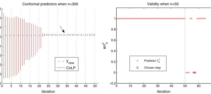
Γ_kε is valid. Moreover the criterion for choosing the CoLP is adapted to variable selection as conformal predictors con-structed here for different values ofλk, k=1, . . . , K bring into play different variables. This is illustrated in Fig. 1

(left) where we constructed the conformal predictors when

n=300. One can observe that all the conformal predictors are valid since they contain the true value of the labelynew. Hence our construction is suitable when the sample size is larger than the number of variables (i.e., n > p) but may be not appropriated whenp≥n. Figure1(right) shows an example where almost all the constructed conformal predic-torsΓ_kε, k=1, . . . , K, using the above algorithm are valid. Only six are not. One of them is the selected CoLP (itera-tion 57 in Fig.1(right)) which corresponds to the smallest predictor. In such cases (p≥n), a correction can be made and other choices for the accuracy measure are possible. We discuss this criterion in Sect.7. Let us add that we only il-lustrated the validity of the conformal predictors in Fig.1

(right) as the unstable zone (on the right side of the verti-cal line) makes the representation hard to be analyzed. More details are given in Sect.7.

Remark 4 In Step 1 of Algorithm1, we use the LARS al-gorithm for its ability to generate a small number of tuning parameter values of interest. It is an important aspect as it considerably reduces the computational cost. On-line sions could be implemented by plugging in an on-line ver-sion of the LASSO solution as in the paper by Garrigues and El Ghaoui (2008) and more recently by Langford et al. (2009) and Shalev-Shwartz and Tewari (2009). The analysis of such on-line versions is the object of work under progress.

Fig. 1 (Color online) Left: Conformal predictorsΓ_kεevolution through the iterations of the LASSO modification of the LARS algorithm when

n=300 (the first iteration corresponds toλmax and the last one

cor-responds toλmin). The CoLP is drawn in a large cyan line. It

corre-sponds to the 34-th iteration and is marked by the arrow. The horizon-tal dashed blue line corresponds to the value ofynew. Right: Validity

analysis (errε

n) of the conformal predictorsΓkεthrough the iterations of

the LASSO modification of the LARS algorithm whenn=50 (the first iteration corresponds toλmax and the last one corresponds toλmin).

The CoLP is marked by a black square and corresponds to the 57-th iteration. The vertical line represents a separation between a stable and an unstable zone

6 Extension to others procedures

In this section we generalize the construction of the con-fidence predictor to a family of estimators which includes selection-type methods as the Elastic-Net (Zou and Hastie

2005) and the Smooth-Lasso (Hebiri 2008). As for CoLP (Sect.4), we are interested in two properties of estimators: the piecewise linearity w.r.t. the responsey (to easily com-pute the nonconformity scores αi, i=1, . . . , n), and the piecewise linearity w.r.t. the tuning parameterλ(Rosset and Zhu2007) (to reduce computational effort by using a modi-fication of the LARS algorithm).

We use the same notation as in Sect.3 for the LASSO estimator. Set β(x,ˆ y)to be an estimator of the regression vectorβ based on x and y. Let alsos be the sign vector of the estimatorβ(x,ˆ y)(the components ofscan equal zero if the corresponding regression coefficients equal zero). On the other hand, using the notation in Sect.4, we setμˆ =xβ(ˆx,y)

where this timeβ(ˆx,y)is based on the augmented datasetx

andy.

Assumption 1 The estimatorμˆ can be written as: ˆ

μ=U (x, s)y+V (x, s), (13) where U (·) and V (·) are piecewise constant functions w.r.t.y.

As soon as Assumption1holds, we can construct a confor-mal predictor corresponding to the estimatorμˆ. Then many

estimators can be considered. The CoLP and CoRP obvi-ously belong to this class of predictors and we introduce here the Conformal Elastic Net Predictor (CENeP) which is a conformal predictor constructed based on the Elastic-Net modification of the LARS instead of the LASSO one (Step 1 in Algorithm1). Nevertheless, let us first mention that the functionsU (·)andV (·)in the CoLP construction induce the datasetxk instead ofx, where k is one step of the LASSO modification of the LARS algorithm. Then these functions map into a smaller space. For this reason, we will note for such iterative methodsu(·)andv(·)instead ofU (·)

andV (·), but we mention thatUandV can easily be recon-stituted usingu andv by adding, if necessary zeros to the proper places. Now letβˆbe the Elastic-Net estimator (Zou and Hastie2005). Based on the dataset(x,y), this estimator is defined by ˆ β(x,y)=argmin β∈Rp n−1 i=1 yi−xiβ 2 +λ p j=1 |βj| +ν p j=1 β_j2,

whereλ≥0 andν≥0 are two tuning parameters. We note

sits sign vector. Similarly to the LASSO we use a modifi-cation (the Elastic-Net here) of the LARS algorithm to it-eratively computeK >0 solutions β¯1, . . . ,β¯K (analogues to (5)), which easily provideKsolutions of the above min-imization problem by setting to zero the components cor-responding to non active variables. Note that for eachk∈ {1, . . . , K}, the vectorβ¯kis a|Ak|-dimensional vector given

by ¯

βk=xk(xkxk+νkIk)−1xky−λkxk(xkxk)−1sk,

wheresk is the sign vector at thek-th step of the Elastic-Net modification of the LARS algorithm andλk andνk are the tuning parameters evaluated at this step. Finally, follow-ing the same reasonfollow-ing as for the LASSO, Assumption 1

holds with the functions u(xk, sk)=xk(x_kxk +νkIk)−1x_k andv(xk, sk)= −λkxk(xkxk)−1sk, where Ik is the|Ak| × |Ak| identity matrix. In the same way, we can also define the Conformal Smooth Lasso Predictor (CoSmoLaP) based on a Smooth-Lasso modification of the LARS algorithm (Hebiri 2008). Here u(xk, sk)=xk(x_kxk+νkJk)−1x_k and v(xk, sk)= −λkxk(x_kxk)−1sk. The difference between the CoSmoLaP definition the CENeP one is the identity matrix

Ik which is replaced by the |Ak| × |Ak| matrix Jk whose components are such that(Jk)i,i=1 ifi=1 ori= |Ak|and (Jk)i,i =2 otherwise. Moreover for (i, j )∈ {1, . . . ,Ak}2 withi =j, we have(Jk)i,j = −1 if |i−j| =1 and zero otherwise. Note that the definition of Jkmakes the CoSmo-LaP more appropriated to model with correlation between successive variables.

As for CoLP, we can define the nonconformity score

α=(α1, . . . , αn) of an expected label y associated to the estimatorμˆ as follows:

α(y):= |y− ˆμ| = |(I−U (x, s))y−V (x, s)| = |A+B y|,

whereA=(a1, . . . , an)andB=(b1, . . . , bn)with

A:=(I−U (x, s)) (y1, . . . , yn−1,0)−V (x, s), B:=(I−U (x, s)) (0, . . . ,0,1),

and I is then×nidentity matrix. The quantitiesAandBare the analogues ofAk andBk respectively, when we consid-ered the CoLP at the transition pointλk, k=1, . . . , K. Then replacingAkandBk by respectivelyAandBin Step 2.a of Algorithm1, we obtain the conformal predictors associated to the estimatorμˆ.

Note that the dependency in the tuning parameter, notedλ, can be included inU (x, s)(as for CoRP) or V (x, s) or in both of them (as for the CoLP). For instance, in the con-struction of the CoLP, this dependency is underlined in the matrixxk and the sign vectorsk as they were computed by the LARS algorithm for a specified valueλk of the tuning parameterλ.

To evaluate the computational cost of the proposed algo-rithm, three main points should be taken into account. First, one run of the LARS algorithm requires the same cost as the computation of the least square estimation. Then we have to consider the number of conformal predictors we have to con-struct: each value of the tuning parameterλprovides a con-formal predictorΓλusing the algorithm described in Sect.5.

The final conformal predictorΓopt is then the one with the minimal length. As for the CoRP, the main problem is how manyλ’s do we have to test? One way is to use a grid of value forλwhich lets open the question of the choice of the grid and the window of this grid.

On the other hand, we saw that the LARS algorithm allows to reduce considerably the number of tuning meters to be considered. Indeed the grid of tuning para-meters values is directly described by the transition points

λ1, . . . , λK obtained from the run of the LARS algorithm. Finally, let us consider the construction of the conformal predictor itself: this point has been treated by Vovk et al. (2005, Chaps. 2.3 and 4.1). It turns out that sparse conformal predictors and in particular the CoLP require computation timeO(n2)which can be further reduced toO(nlog(n)).

7 Experimental results

In this section we present the experimental performance of the Sparse Conformal Predictors (SCP) with respect to their validity, their accuracy and also their selection power. As a benchmark, we use the CoRP2for its validity and accuracy and the original LASSO and Elastic-Net estimators for their selection3power.

Three SCPs are considered: the Conformal Lasso Predic-tor (CoLP was introduced in Sects.4and5) and the Confor-mal Elastic Net Predictor (CENeP was described in Sect.6). The last SCP called Conformal Ridge Lasso Predictor (CoR-LaP) is a mix of the CoRP and the CoLP. To construct the CoRLaP, we use the variables selected by the LASSO mod-ification of the LARS algorithm (Step 1 in Algorithm1 de-scribed in Sect.5). Then we use these variables to construct a CoRP. This conformal predictor can be seen as a restricted CoRP. All conformal predictors are constructed with confi-dence level 1−ε=90%.

7.1 Synthetic data

We consider four simulated datasets from the linear regres-sion model

y=Xβ+σ ξ,

withβ∈R50, and

X=(X1, . . . ,X50)∈R50, ξ∼N(0,1).

2_{We construct the CoRP associated to same tuning parameters as the} CoLP (i.e., the transition pointsλk observed in Sect.5). Note that the

performance would not be altered as conformal predictors according to this method are almost embedded and changes sensitively while the tuning parameter varies (Vovk et al.2005, p. 39).

3_{We use a BIC-type criterion to select the optimal tuning parameter.} Such a criterion is adapted to variable selection.

Fig. 2 (Color online) Analysis of conformal predictors length (y-axis)

through the LASSO modification of the LARS algorithm iterations (x-axis: the first iteration corresponds toλmax and the last one

cor-responds to λmin) in Example (c)[300/1] (top left) and in

Exam-ple (c)[50/1] (top right). The iteration associated to the CoLP is

marked by a blue star. Predictors which are non valid are marked by a black circle. The panel of bottom shows the lengths of intervals in a logarithmic scale associated to the same Example (c)[50/1] dis-played in the top right panel

Hencep=50 through the simulations. Noise levelσand the sample sizenare left free. They will be specified during experiments.

Example (a) [n/σ]: Very Sparse and Correlated. Here only

β1 is nonzero and equals 5. Moreover, the design cor-relation matrix is described by j,k=exp(−|j −k|) for (j, k)∈ {15, . . . ,35}2 andj,k=I(j =k)otherwise whereI(·)is the indicator function.

Example (b) [n/σ]: Sparse and Correlated. Correlations are defined as in Example (a) and the regression vector is given byβj = −5+0.2j forj =1, . . . ,5;βj =4+0.2j forj=10, . . . ,25 and zero otherwise.

Example (c) [n/σ]: Sparse and Highly correlated. We have

βj =5 for j ∈ {1, . . . ,15} and zero otherwise. We con-struct three groups of correlated variables: j,j =1 for everyj∈ {1, . . . , p}; forj =k,j,k≈1 (actuallyj,k=

1

1+0.01, due to an extra noise variable) when(j, k)belongs

to{1, . . . ,5}2,{6, . . . ,10}2and{11, . . . ,15}2and zero oth-erwise.

Example (d) [n/σ]: Non Sparse and Correlated. Hereβj= 3+0.2j for j ∈ {1, . . . , p} and the correlations are de-scribed byj,k=exp(−|j−k|)for(j, k)∈ {1, . . . , p}2.

We consider separately the three points of interest: accu-racy, validity and selection.

Accuracy. First of all, let us consider the length of the pre-dictorsΓ_kε, k=1, . . . , K obtained at the end of Step 2 in Algorithm 1 described in Sect. 5. We recall that each of these predictors is associated to an iteration of a modifi-cation of the LARS algorithm, that is the transition points

λk, k=1, . . . , K. Figure2illustrates the predictors lengths for the construction of the CoLP, when applied to Exam-ple (c)[n/1] withn=300 andn=50. Whenn=300, we note that the length of the Γ_kεs sensitively changes from

Table 1 Mean lengths [with

precision±95%] of the CoRP, CoLP, CoRLaP, CENeP, the Early-Stopped CoLP and the 2-PN CoLP based on 500 replications EXAMPLE σ CORP COLP CORLAP CENEP (a)[300/σ] 1 3.7±0.1 3.2±0.1 3.1±0.1 3.2±0.1 (a)[50/σ] 3 13.4±0.3 7.4±0.3 4.7±0.3 7.1±0.3 (b)[300/σ] 1 8.5±0.1 3.4±0.1 3.3±0.1 3.4±0.1 (b)[50/σ] 1 20.3±0.1 3.9±0.1 2.3±0.1 3.7±0.1 (b)[20/σ] 1 101.2±0.1 52.5±0.1 17.2±0.1 37.6±0.1 (c)[300/σ] 1 3.9±0.1 3.4±0.1 3.2±0.1 3.3±0.1 (c)[300/σ] 3 11.0±0.3 10.1±0.3 9.6±0.3 9.7±0.3 (c)[300/σ] 10 34.3±0.9 33.0±0.9 31.8±0.9 32.2±0.9 (d)[300/σ] 10 286.5±0.9 70.2±0.9 36.0±0.9 54.0±0.9 EXAMPLE σ CORP COLP STOPPED-COLP 2-PN-COLP (a)[50/σ] 3 13.1±0.3 7.2±0.3 9.1±0.3 9.5±0.3 (b)[50/σ] 1 20.7±0.1 3.9±0.1 5.5±0.1 5.9±0.1 (b)[50/σ] 10 55.3±0.9 32.1±0.9 46.2±0.9 48.7±0.9 (c)[20/σ] 3 28.3±0.3 7.44±0.3 13.2±0.3 14.1±0.3 (d)[20/σ] 10 233.0±0.9 115.3±0.9 164.1±0.9 170.2±0.9

one iteration to the following and that the larger predic-tor has a reasonable length compared to the smallest one (about 10 times larger). Then the construction is stable. We also observe that in the neighborhood of the optimal iter-ation (that is iteriter-ation 20), the conformal predictors have approximately the same size. Such an observation can also be made when we take a look at Fig.1(left) when applied to Example (b)[300/1]. On the other hand, whenn=50, it appears that the predictors length grows drastically at some iteration (around iteration 85). We even cannot compare the lengths of the bigger and smaller predictors (more than 104 times larger). In the same time, it seems that the construc-tion becomes unstable as strong variaconstruc-tions often happen af-ter this iaf-teration 85. We will consider in the next point the validity of these predictors. However let us mention that in Example (c)[50/1], the CoLP which is the smallestΓ_kεand then the selected predictor is not valid (in Fig.2(right), the selected predictor at iteration 93 is not valid). This aspect can also be observed in Fig.1(right) (the graph corresponds to Example (b)[50/1]) where the selected CoLP at iteration 57 is not valid. Similar strong variations of the correspond-ing predictors lengths would have been observed after iter-ation 49 if we have provided a graph as Fig.2(right).

Now let us compare the accuracy of the final conformal predictors obtained at the end of Step 3 in Algorithm 1

while using the different methods or different values for the setting parameters. Table1 sums up the obtained results. First of all, an important remark is that all Sparse Con-formal Predictors (CoLP, CoRLaP, CENeP, . . .) are more

accurate than the CoRP. Indeed, the length of the SCPs are most of the time more than twice smaller than the CoRP one. However when we treat problems with both small level of noise and big sample size, it happens that the gain of accuracy is limited as can be seen in Example (a)[300/1] and Example (c)[300/1]. In such situations, one should all the same mention that all provided conformal predictors are accurate. Through these observations we conclude that SCPs exploit favorably the sparsity in order to improve the accuracy of conformal predictors. Comparing the accuracy of the CoLP, the CoRLaP and the CENeP, it turns out that the CoRLaP is the more accurate SCP, whereas the CoLP is the less accurate one. In the other hand, let us now con-sider the influence of the setting parameters on the accu-racy. It seems to be clear that the smaller the sample size is or the higher the noise level is, the larger the length of the conformal predictors is (see Example (b)[n/1] and Exam-ple (c)[300/σ] respectively). Noise level and sample size seems to be the more influential parameters on the accu-racy of the predictors. Finally except for the case where the model is not sparse (Example (d)[n/σ]), one can ob-serve that the sparsity is not a crucial parameter on the ac-curacy. This can be illustrated through the obtained results on Example (a)[300/1], Example (b)[300/1] (for which the dataset is built with the same correlation matrix as in Example (a)) and Example (c)[300/1].

Validity. Now, we consider the validity of the selected pre-dictors (cf. Step 3 in Algorithm1). As shown in Table2, we observe that variations on the noise level, the vari-ables correlations and the sparsity of the model do not

Table 2 Validity frequencies

[with precision±95%] of the CoRP, CoLP, CoRLaP, CENeP, the Early-Stopped CoLP and the 2-PN CoLP based on 1000 replications EXAMPLE σ CORP COLP CORLAP CENEP (a)[300/σ] 1 0.899±0.019 0.886±0.020 0.854±0.022 0.882±0.020 7 0.894±0.019 0.908±0.018 0.894±0.019 0.899±0.019 15 0.893±0.019 0.893±0.019 0.879±0.020 0.887±0.020 (b)[300/σ] 1 0.901±0.018 0.895±0.019 0.889±0.020 0.892±0.019 (c)[300/σ] 1 0.900±0.019 0.900±0.019 0.891±0.019 0.901±0.018 (d)[300/σ] 1 0.892±0.019 0.895±0.019 0.895±0.019 0.895±0.019 (a)[50/σ] 3 0.887±0.020 0.668±0.029 0.414±0.030 0.789±0.025 (a)[20/σ] 3 0.865±0.021 0.596±0.030 0.304±0.028 0.685±0.029 EXAMPLE σ CORP COLP STOPPED-COLP 2-PN-COLP (a)[50/σ] 7 0.853±0.022 0.620±0.030 0.815±0.024 0.881±0.020 (b)[50/σ] 1 0.854±0.022 0.624±0.030 0.814±0.024 0.907±0.018 (c)[20/σ] 15 0.875±0.020 0.608±0.030 0.769±0.026 0.893±0.019 (d)[20/σ] 1 0.900±0.019 0.602±0.030 0.793±0.025 0.892±0.019

perturb the validity whereas the sample size relatively to the dimension p does. When n=300> p, all the pro-cedures seem to be quite similar and produce good pre-dictors. In the other cases, i.e., when n=p =50 and

n=20< p, the selected confidence predictors have worst performance than expected (validity with smaller propor-tion than 1−ε=90%). Moreover, Sparse Confidence Pre-dictors perform worst than the CoRP as observed in Ta-ble2. As pointed in the accuracy part, one explication can be observed in Fig.2as the selected predictor which also is not valid (iteration 93) corresponds to an iteration in the unstable zone (that is, after iteration 85). Then in order to reduce the gap between SCP and CoRP in the casesp≥n, we suggest to modify the selection criterion in Step 3 in two ways. (i) Early Stopping CoLP: do not consider (and do not construct) all the conformal predictorsΓ_kε. Stop the construction of the predictorsΓ_kε as soon as the length of

Γ_kε (predictor at iterationk) has a length at least 10 times larger thanΓ_kε₋₁; (ii)N Previous Neighbors CoLP: we can enforce the Early Stopping rule by considering as final pre-dictor:Γ_optε =_{j:0≤k−j <N}Γ_jε, wherekis the index of the (selected) smallest predictor andNis the number of neigh-bors we consider. Table1exemplifies the performance of these corrected versions of the CoLP according to their ac-curacy. Obviously both of the above rules provide slightly larger predictors than the original CoLP. In the same time we observe that the Early Stopping CoLP and 2 Previ-ous Neighbors CoLP are still much more accurate than the CoRP. Note further thatN Previous Neighbors rule does not alter a lot the accuracy of the Early Stopping CoLP (see Table1). This is due to the fact that the Early Stopping rule ensures that we are in the stable zone (cf. Fig.2(right) and Fig.1(right)). Moreover, note that theN Previous

Neigh-bors rule does not neither alter the selection properties of the Early Stopping CoLP asΓ_kεis usually constructed with more variables thanΓ_jε whenj < k. Finally Table2sums up the performance of the early-stopped CoLP and the 2-PN CoLP in term of validity. We observe the good adapta-tion of both methods to the casep=nand we remark that 2-PN CoLP nicely produce valid predictor even in the case

p > n. This improvement in the term of validity can also be illustrated by Fig.1(right) where we observe that in Ex-ample (b)[50/1], the early-stopped CoLP is valid whereas the original CoLP is not.

Selection. Here, we are concerned by the selection ability of Sparse Conformal Predictors. First of all, note that the se-lected variables in SCPs are directly linked to the selection ordering through the iterations of the LASSO or Elastic-Net modification of the LARS algorithm. Then, if the used modification of the LARS algorithm fails to recover the true model, we cannot hope to get a predictor which con-tains only the true variables. Figure3 illustrates the evo-lution of the variable selection of CoLP, CoRLaP and the LASSO on one hand and the CENeP and the Elastic-Net on the other hand, in Example (b)[300/1]. It turns out that CoLP and CENeP select larger model that expected (that is, some noise variables are selected), as the LASSO and the Elastic-Net do. Moreover CoRLaP uses to select a smaller subset of variables than the CoLP. Then it often produces a better variable selection performance than the other meth-ods. It often provides closer model to the true one. Com-pared to the LASSO, it seems that the CoLP and the CoR-LaP perform better in this example. However, we can not conclude to the superiority of the CoLP on the LASSO in term of variable selection. A similar conclusion can be

Fig. 3 (Color online) Variable selection analysis for the CoLP, the

CoRLaP and the CENeP in Example (b)[300/1] (variables 1 to 5 and 10 to 25 are relevant; see variables in dark blue on the plot). On the left, we consider the CoLP and the CoRLaP selected variables (x-axis) with respect to the LASSO modification of the LARS algorithm iter-ations (y-axis: the first iteration corresponds toλmax and the last one

corresponds toλmin). On the right, we consider the CENeP selected

variables (x-axis) with respect to the Elastic-Net modification of the LARS algorithm iterations (y-axis: the first iteration corresponds to

λmax and the last one corresponds toλmin). The selected iteration is

marked by red diamonds for the CoLP, green squares for CoRLaP and black squares for the CENeP

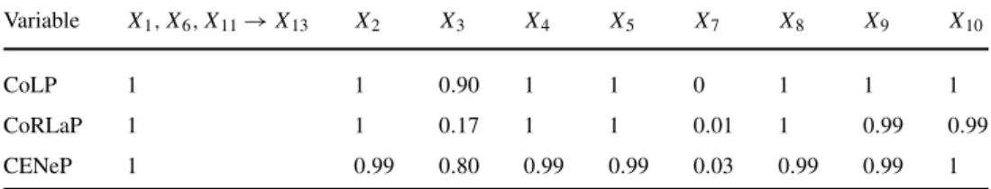
Table 3 Selection frequency of

each variable by the different SCPs on 150 random permutations of the House Boston dataset with (p=13 and

n=506)

Variable X1, X6, X11→X13 X2 X3 X4 X5 X7 X8 X9 X10

CoLP 1 1 0.90 1 1 0 1 1 1

CoRLaP 1 1 0.17 1 1 0.01 1 0.99 0.99

CENeP 1 0.99 0.80 0.99 0.99 0.03 0.99 0.99 1

given when we compare the CENeP and the Elastic-Net. Nevertheless, the CENeP seems to select little larger mod-els than the Elastic-Net. Finally, analogously to the superi-ority of the Elastic-Net compared to the LASSO, we can re-mark that the CENeP manages to have better selection per-formances compared to the CoLP and the CoRLaP when a group structure may exist between different variables (for instance in Example (d)[n/σ]). This is due to the LASSO modification of the LARS algorithm which uses to select some noise variables before relevant ones in such cases. 7.2 Real data

We apply SCPs on 150 random permutations of the House Boston dataset,4 in which we randomly choose one row to be the new pair (xnew, ynew). The original dataset con-sists of 506 observations with 13 variables. First Table 3

displays the obtained variable selection results. We note that almost all SCPs are constructed without the variable

4_{The data and their description are available athttp://archive.ics.uci.}

edu/ml/datasets/Housing.

X7=(x1,7, . . . , x505,7). This variable is selected with fre-quencies lower than 3%. The CoRLaP also does not con-sider the variableX3as relevant with a frequency equal to 17%. Conforming to Sect.7.1, we would better considerX3 irrelevant as the CoRLaP uses to produce better performance when variable selection is in concern. Then we conclude that the proportion of non-retail business acres per town and the proportion of owner-occupied units built prior to 1940 do not interfere in the value of owner-occupied homes. A gen-eral observation is that variable selection improves the ac-curacy of conformal predictors (as already seen in Table1). Here, the median lengths of the CoLP, the CoRLaP and the CENeP are respectively 13.61, 13.50 and 13.58, whereas CoRP length is 14.45.

To consider a high dimensional setting we use the same trick as in the paper by Bühlmann and Hothorn (2010). For this purpose, we look at a synthetically enlargement of the Boston Housing dataset. We add 483 additional, in-effective noise predictor variablesXadd ∼N483(0,I). The new design matrix X has then p=500 columns or vari-ables with at most 13 effective predictors. We fix this

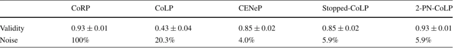
ma-Table 4 Validity frequencies (with precision±95%) and noise variables selection (variablesX14toX500) of the CoRP, CoLP, CENeP, the Early-Stopped CoLP and the 2-PN CoLP based on the augmented Boston Housing dataset (p=500 andn=50)

CoRP CoLP CENeP Stopped-CoLP 2-PN-CoLP

Validity 0.93±0.01 0.43±0.04 0.85±0.02 0.85±0.02 0.93±0.01

Noise 100% 20.3% 4.0% 5.9% 5.9%

trix. In the sequel, we arbitrarily chose 50 examples among the available 506 rows of this matrixX. As a consequence we have constructed two datasets: a training set with 50 instances and a test set with 456 instances. Each instance is a 500-dimensional vector. In this high dimensional set-ting, we apply the SCPs on 100 random permutations of the training dataset. Each time, we randomly chose one row in the test dataset to be the new pair(xnew, ynew). We study the behavior of the CoRP, the CoLP, the CENeP, the early-stopped-CoLP and of the 2-PN CoLP in such a frame-work.

As observed on synthetic data, all of the CENeP, the early-stopped-CoLP and the 2-PN CoLP have better perfor-mance than the original CoLP (see Table4). We also observe that the better performance is reached by the 2-PN CoLP and the CoRP with a validity equal to 0.93 (this is better than the expected validity level). However, an important point is that the 2-PN CoLP has also the advantage of producing a sparse predictor whereas the CoRP does not.

As for the accuracy, let us remark that the lengths of the SCPs are much smaller than the CoRP length. Indeed the median lengths of the CoLP, the CENeP, the early-stopped-CoLP and the 2-PN early-stopped-CoLP are respectively 1.5, 8, 8 and 8, whereas the CoRP’s length equals 19. This observation ad-vocates for the use of the 2-PN CoLP.

According to the selection task, we observe in Table 4

(last line) that at most 6% of the additional noise variables are selected by the SCPs (except the CoLP which selects more than 20% of these irrelevant variables). Concerning the original variables, onlyX1, X4, X6, X11, X12 andX13are selected. This at least confirms that the proportion of non-retail business acres per town and the proportion of owner-occupied units built prior to 1940 (X3andX7respectively) do not interfere in the value of owner-occupied homes as observed above in the casep≤n.

Remark 5 For comparison, Sparse Conformal Predictors have also been applied on the same setting as above but without the 483 additional noise predictor variables. It turns out that also in this situation the 2-PN CoLP has a valid-ity frequency equal to 0.92 which is larger than expected (0.9). The 2-PN CoLP seems to provide better performance than the CoRP and the CoLP in this dataset. Moreover, the same variablesX1, X4, X6, X11, X12have been considered as relevant.

8 Conclusion

In this paper, we introduced a new family ofl1regularized conformal predictors termed Sparse Conformal Predictors. We then focused on LASSO and Elastic-Net versions of these Sparse Conformal Predictors and illustrated their per-formance in terms of accuracy, validity and variable selec-tion. The experiments reported in the paper show that SCPs are valid and nicely exploit the sparsity of the model when the sample size is larger than the number of variables (i.e., whenn > p). We also provided a way to adopt these sparse predictors to the casep≥nthrough a pair of rules we called Early Stopping andN Previous Neighbors rules. It turns out that a 2 Previous Neighbors rule is really attractive. Indeed, even in a high dimensional setting, it allows to achieve good performance for all of the criteria: validity, accuracy and se-lection.

Several extensions of this work can be explored such as the construction of SCP with Adaptive LASSO (Zou

2006) or the adaptation of SCPs in the generalizedl1 reg-ularized linear model, using algorithmic developments pre-sented for instance by Park and Hastie (2007). These top-ics, as well as the combination of the conformal predic-tors with other sparsity inducing procedures, such as the exponentially weighted aggregate (Dalalyan and Tsybakov

2007,2008) or grouped variable Lasso (Yuan and Lin2006; Chesneau and Hebiri2008), are interesting avenues for

fu-ture research.

Acknowledgements We would like to thank the Referees for their helpful comments and suggestions. They helps us to improve signifi-cantly this revised version of the paper. We also would like to thank Professors Arnak Dalalyan and Nicolas Vayatis for insightful com-ments.

References

Bühlmann, P., Hothorn, T.: Twin boosting: improved feature selection and prediction. Stat. Comput. (2010, this issue)

Bunea, F., Tsybakov, A., Wegkamp, M.: Sparsity oracle inequalities for the Lasso. Electron. J. Stat. 1, 169–194 (2007)

Casella, G., Berger, R.L.: Statistical Inference. Duxbury, N. Scituate (2001)

Chen, S.S., Donoho, D.L.: Atomic decomposition by basis pursuit. Technical Report (1995)

Chesneau, Ch., Hebiri, M.: Some theoretical results on the grouped variables Lasso. Math. Methods Stat. 17, 317–326 (2008)

Dalalyan, A., Tsybakov, A.: Aggregation by exponential weighting and sharp oracle inequalities. In: Learning Theory. Lecture Notes in Comput. Sci., vol. 4539, pp. 97–111. Springer, Berlin (2007) Dalalyan, A., Tsybakov, A.: Aggregation by exponential weighting,

sharp pac-bayesian bounds and sparsity. Mach. Learn. 72, 39–61 (2008)

Efron, B., Hastie, T., Johnstone, I., Tibshirani, R.: Least angle regression—with discussion. Ann. Stat. 32, 407–499 (2004) Friedman, J., Hastie, T., Höfling, H., Tibshirani, R.: Pathwise

coordi-nate optimization. Ann. Appl. Stat. 1, 302–332 (2007)

Garrigues, P., El Ghaoui, L.: An homotopy algorithm for the lasso with online observations. In: Neural Information Processing Systems (Nips), vol. 21, pp. 489–496. MIT Press, Cambridge (2008) Györfi, L., Kohler, M., Krzyzak, A., Walk, H.: A Distribution-Free

Theory of Nonparametric Regression. Springer Series in Statis-tics. Springer, New York (2002)

Hebiri, M.: Regularization with the smooth-lasso procedure. Technical Report (2008)

Huang, C., Cheang, G.L.H., Barron, A.: Risk of penalized least squares, greedy selection and l1 penalization for flexible function libraries. Preprint (2008)

Kim, S.J., Koh, K., Lustig, M., Boyd, S., Gorinevsky, D.: An interior-point method for large-scale l1-regularized least squares. IEEE J. Sel. Top. Signal Process. 1, 606–617 (2007)

Knight, K., Fu, W.: Asymptotics for lasso-type estimators. Ann. Stat.

28, 1356–1378 (2000)

Langford, J., Li, L., Zhang, T.: Sparse online learning via truncated gradient. J. Mach. Learn. Res. 10, 777–801 (2009)

Meinshausen, N., Bühlmann, P.: High dimensional graphs and variable selection with the lasso. Ann. Stat. 34, 1436–1462 (2006) Osborne, M., Presnell, B., Turlach, B.: On the LASSO and its dual.

J. Comput. Graph. Stat. 9, 319–337 (2000a)

Osborne, M.R., Presnell, B., Turlach, B.A.: A new approach to variable selection in least squares problems. IMA J. Numer. Anal. 20, 389– 403 (2000b)

Park, M.Y., Hastie, T.:L1-regularization path algorithm for generalized linear models. J. R. Stat. Soc., Ser. B, Stat. Methodol. 69, 659–677 (2007)

Rosset, S., Zhu, J.: Piecewise linear regularized solution paths. Ann. Stat. 35, 1012–1030 (2007)

Santosa, F., Symes, W.W.: Linear inversion of band-limited reflection seismograms. SIAM J. Sci. Stat. Comput. 7, 1307–1330 (1986)

Shalev-Shwartz, S., Tewari, A.: Stochastic methods for1regularized loss minimization. In: Proceedings of the 26th International Con-ference on Machine Learning. Omnipress, Montreal (2009) Tibshirani, R.: Regression shrinkage and selection via the lasso. J. R.

Stat. Soc., Ser. B 58, 267–288 (1996)

Tibshirani, R., Saunders, M., Rosset, S., Zhu, J., Knight, K.: Sparsity and smoothness via the fused lasso. J. R. Stat. Soc., Ser. B, Stat. Methodol. 67, 91–108 (2005)

Vapnik, V.: Statistical Learning Theory. Adaptive and Learning Sys-tems for Signal Processing, Communications, and Control. Wiley, New York (1998)

Vovk, V.: Asymptotic optimality of transductive confidence machine. In: Algorithmic Learning Theory. Lecture Notes in Comput. Sci., vol. 2533, pp. 336–350. Springer, Berlin (2002a)

Vovk, V.: On-line confidence machines are well-calibrated. In: Pro-ceedings of the Forty-Third Annual Symposium on Foundations of Computer Science, pp. 187–196. IEEE Computer Society, Los Alamitos (2002b)

Vovk, V., Gammerman, A., Saunders, C.: Machine-learning applica-tions of algorithmic randomness. In Proceedings of the 16th In-ternational Conference on Machine Learning, pp. 444–453. ICML (1999)

Vovk, V., Gammerman, A., Shafer, G.: Algorithmic Learning in a Ran-dom World. Springer, New York (2005)

Vovk, V., Nouretdinov Ilia, G., Gammerman, A.: On-line predictive linear regression. Technical Report (2007)

Yuan, M., Lin, Y.: Model selection and estimation in regression with grouped variables. J. R. Stat. Soc., Ser. B, Stat. Methodol. 68, 49– 67 (2006)

Zhao, P., Yu, B.: On model selection consistency of Lasso. J. Mach. Learn. Res. 7, 2541–2563 (2006)

Zou, H.: The adaptive lasso and its oracle properties. J. Am. Stat. As-soc. 101, 1418–1429 (2006)

Zou, H., Hastie, T.: Regularization and variable selection via the elastic net. J. R. Stat. Soc., Ser. B, Stat. Methodol. 67, 301–320 (2005) Zou, H., Hastie, T., Tibshirani, R.: On the “Degrees of Freedom” of

the lasso. Ann. Stat. 35, 2173–2192 (2007). URLciteseer.ist.psu. edu/766780.html