Copyright by
Dylan Zachary Anderson 2015
The Thesis Committee for Dylan Zachary Anderson
Certifies that this is the approved version of the following thesis:
Supervised Gamma Process Poisson Factorization
APPROVED BY
SUPERVISING COMMITTEE:
Joydeep Ghosh, Supervisor
Supervised Gamma Process Poisson Factorization
by
Dylan Zachary Anderson, B.S.E.E.
Thesis
Presented to the Faculty of the Graduate School of the University of Texas at Austin
in Partial Fulfillment of the Requirements
for the Degree of
Master of Science in Engineering
The University of Texas at Austin May 2015
Supervised Gamma Process Poisson Factorization
by
Dylan Zachary Anderson, M.S.E. The University of Texas at Austin, 2015
SUPERVISOR: Joydeep Ghosh
This thesis develops the supervised gamma process Poisson factorization (S-GPPF) framework, a novel supervised topic model for joint modeling of count matri-ces and document labels. S-GPPF is fully generative and nonparametric: document labels and count matrices are modeled under a unified probabilistic framework and the number of latent topics is controlled automatically via a gamma process prior. The framework provides for multi-class classification of documents using a generative max-margin classifier. Several recent data augmentation techniques are leveraged to provide for exact inference using a Gibbs sampling scheme.
The first portion of this thesis reviews supervised topic modeling and several key mathematical devices used in the formulation of S-GPPF. The thesis then introduces the S-GPPF generative model and derives the conditional posterior distributions of the latent variables for posterior inference via Gibbs sampling. The S-GPPF is shown to exhibit state-of-the-art performance for joint topic modeling and document classi-fication on a dataset of conference abstracts, beating out competing supervised topic models. The unique properties of S-GPPF along with its competitive performance make it a novel contribution to supervised topic modeling.
Contents
Abstract . . . iv
List of Tables . . . vii
List of Figures . . . viii
Chapter 1. Introduction . . . 1
1.1 Problem Statement . . . 1
1.2 Contributions of this Thesis . . . 2
Chapter 2. Background . . . 5
2.1 Notation . . . 5
2.2 Topic Modeling . . . 6
2.3 Useful Distributions and Results . . . 12
2.4 Hinge Loss and Location-mixture of Normals . . . 16
Chapter 3. Supervised Gamma Process Poisson Factorization . . . 18
3.1 Generative Process . . . 18
3.2 Inference . . . 20
3.3 Training Phase . . . 26
3.4 Test Phase . . . 27
Chapter 4. Experiment Analysis . . . 28
4.2 ACM Conference Abstracts Classification . . . 32
Chapter 5. Conclusion . . . 40
5.1 Practical Suggestions . . . 40
5.2 Discussion and Future Work . . . 42
Appendices . . . 44
Appendix A. Proofs of Lemmas . . . 45
Appendix B. Conditional Posterior Derivations . . . 49
List of Tables
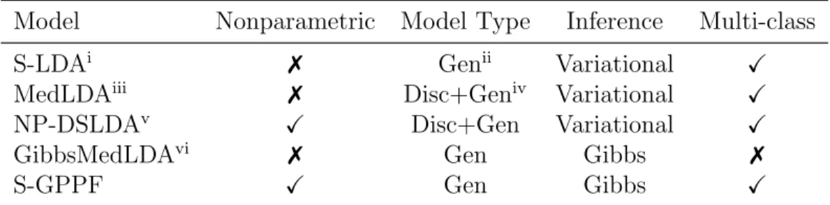
1.1 S-GPPF and Other Related Models . . . 3 4.1 Top topic for each conference . . . 39
List of Figures
2.1 Plate model for Latent Dirichlet Allocation . . . 8
2.2 Plate model for supervised latent Dirichlet allocation . . . 9
2.3 Plate model for Gamma Process Poisson Factorization . . . 12
2.4 Alternative constructions of the Negative Binomial distribution . . . . 15
3.1 Plate Diagram of Supervised GPPF . . . 21
4.1 Synthetic block diagonal data . . . 29
4.2 Reconstructed block diagonal X and z matrices . . . 30
4.3 Active topics in synthetic data . . . 31
4.4 Document- and word- topic affinities in synthetic data . . . 32
4.5 Class regression parameters in synthetic data . . . 33
4.6 Document length distribution in ACM conference abstracts . . . 34
4.7 ACM conference abstract statistics . . . 34
4.8 Classification Accuracy vs. Train Size . . . 37
Chapter 1
Introduction
This thesis considers the problem of modeling text and other count data in a fully probabilistic framework. Furthermore, each observation within a dataset is assumed to have a single categorical response variable. The objective is to jointly perform di-mensionality reduction and document class label prediction using the dimensionally-reduced space. This thesis describes the Supervised Gamma Process Poisson Factor-ization (S-GPPF), a fully probabilistic framework to jointly model count observations, latent factors, and observation class labels.
1.1
Problem Statement
Supervised topic modeling seeks to jointly perform dimensionality reduction into a latent topic space and predict document class labels. Some approaches provide su-pervision by labeling each document with its set of topics [Ramage et al., 2009, Rubin et al., 2012]. Other approaches [Mcauliffe and Blei, 2008, Zhu et al., 2009, Chang and Blei, 2009] assume that supervision is provided for a single response variable to be predicted for a given document. The response variable might be real-valued or categorical, and modeled by a normal, Poisson, Bernoulli, multinomial or other dis-tribution (see Chang and Blei [2009] for details). Other works deal with supervision at both the topic and document level [Acharya et al., 2013]. Some examples of docu-ments with response variables are essays with their grades, movie reviews with their numerical ratings, web pages with their number of hits over a certain period of time,
and documents with category labels.
Some supervised topic models [Mcauliffe and Blei, 2008, Chang and Blei, 2009] have found the categorical response variable difficult to model jointly with the latent topics as the resulting inference is intractable. Maximum Entropy Discriminative LDA (MedLDA, Zhu et al. [2009]) address this problem by solving two problems jointly: dimensionality reduction and max-margin classification using the features in the dimensionally-reduced space. MedLDA solves the inference problem via varia-tional approximations. Though the update equations are simple, the approximation negatively affects the empirical performance. Additionally, the model has both dis-criminative and generative components combined in a unified framework, thereby limiting the choice of priors and model flexibility. MedLDA has been extended to Gibbs sampling based inference [Zhu et al., 2013] with a completely generative model. However, it does so at the cost of multi-class response variable modeling. The so-called Gibbs-MedLDA must make use of a one-versus-all (OVA) framework to extend its binary classification to the multi-class setting.
The problem addressed in this thesis is joint modeling of dimensionality reduction and a multi-class response variable. Furthermore, additional properties are imposed upon the model which contribute to its novelty: the model is restricted to be fully generative, non-parametric, and must have exact inference.
1.2
Contributions of this Thesis
This thesis addresses the supervised topic model problem by developing the super-vised gamma process Poisson factorization framework. S-GPPF extends the Poisson factorization model put forth by Zhou et al. [2012] to the supervised setting. S-GPPF explicitly models multiclass document class responses, eliminating the need
Model Nonparametric Model Type Inference Multi-class
S-LDAi 7 Genii Variational X
MedLDAiii 7 Disc+Geniv Variational
X
NP-DSLDAv X Disc+Gen Variational X
GibbsMedLDAvi 7 Gen Gibbs 7
S-GPPF X Gen Gibbs X
iMcauliffe and Blei [2008] iiGenerative iiiZhu et al. [2009] ivDiscriminative+Generative vAcharya et al. [2013] viZhu et al. [2013]
Table 1.1: S-GPPF and Other Related Models
for a one-versus-all framework to extend a binary classification to the multiclass set-ting. Multiclass modeling improves classifier performance, particularly when there is a small amount of labeled data available as jointly modeling classes serves as an in-ductive bias in prediction of the other class labels, as in multi-task learning. S-GPPF is a fully generative model. This greatly expands the model flexibility in generalizing to new data and in providing interpretation for model predictions. S-GPFF is also a non-parametric model, automatically selecting the number of topics from the data. Finally, S-GPPF provides for exact inference via Gibbs sampling. No other supervised topic model provides a completely Bayesian formulation of a max-margin multiclass classification with an unbounded number of topics and closed form inference via Gibbs sampling. These properties are summarized in Table 1.1.
This thesis is organized as follows. In Chapter 2, relevant literature is reviewed and the mathematical machinery used to implement the framework is discussed. Chapter 3 describes the generative model and provides the Gibbs sampling update equations. It also describes running the model in separate training and testing phases and discusses parameter estimation. Chapter 4 uses S-GPPF to factor real data, and shows its empirical performance to be competitive to the state of the art. Finally, Chapter 5
concludes this thesis with a discussion of the work presented as well further avenues of research.
Chapter 2
Background
This chapter provides an overview of related literature and introduces the math-ematical devices used to develop the model and its closed form updates for Gibbs sampling. Note that a proof for each lemma presented can be found in Appendix A or the relevant literature. The chapter is arranged as follows. Section 2.1 introduces the mathematical notations used throughout this thesis as well as some terminology to describe data within the S-GPPF framework. Section 2.2 introduces the broad subject of topic modeling and discusses prominent models for both supervised and unsupervised topic modeling. Section 2.3 provides key results that are necessary for the derivations of the conditional posterior sampling equations for the S-GPPF and introduces uncommon distributions used in the S-GPPF model. Finally, Section 2.4 discusses the formulation of max-margin classifiers and their multiclass extensions in fully generative frameworks.
2.1
Notation
A consistent mathematical notation is adopted throughout this document. Bold, upper [lower] case letters such as A [b] denote matrices [vectors]. The element of a matrix Aat row i, columnj is denoted as aij. The set of real numbers is denoted as R. The set of numbers {x∈ R : x >0} is denoted R+. The set of positive integers
{0,1,2,· · · }is denoted asZ+. IK is used to denote aK×K sized identity matrix. A
asP k
xdk =x.k where the index of the axis that is summed over is replaced with a dot.
The notation x| · · · is used to denote the random variablex given all other variables in the model. The script letter N is used to denote the normal distribution.
Throughout this thesis, data is referred to within the context of text corpora. The smallest unit of discrete data is the word, which is an item from a vocabulary set indexed by {1,· · · , V}. Adocument is a sequence of words. A corpus is a set of documents indexed by {1,· · · , D}. Using text terms for describing data is useful for providing intuition behind modeling state variables. However, S-GPPF is not limited to textual data; the model is readily applied to supervised factorization of generic count matrices.
2.2
Topic Modeling
Topic modeling can be viewed as unsupervised dimensionality reduction and clus-tering of documents in a lower dimensional latent space. Topic modeling posits that underlying a corpus is a set of latent topics. From Blei et al. [2003], “each word is generated from a single topic, and different words in a document may be generated from different topics.” Each topic is a distribution over words and each document is in turn a distribution over topics. The key insight is that given a document about a particular topic or set of topics, the document should predominantly feature words related to those topics. Informally, topics represent the underlying thematic content of a document.
Underpinning the theory of topic modeling is an assumption of exchangeability of documents and words. In other words, the ordering of words within a document and documents within a corpus is inconsequential [Aldous, 1985]. This is clearly a simpli-fying assumption: the order of words in a sentence is paramount to understanding.
The exchageability assumption makes modeling and inference much more straightfor-ward and tractable. To introduce some dependency on the ordering of words, larger discrete units of data such as n-grams can be just as easily modeled under topic modeling. From the De Finetti et al. [1990] representation theorem, a collection of exchangeable random variables has a representation as a mixture distribution. In general, the mixture can be infinite, naturally lending to nonparametric Bayesian methods. This mixture representation motivates the most prolific topic model, latent Dirichlet allocation (LDA, Blei et al. [2003]), which is described in detail in the next section.
2.2.1 Latent Dirichlet Allocation
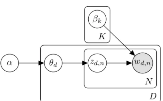
Latent Dirichlet Allocation [Blei et al., 2003] treats documents as a mixture of topics, which in turn are defined by a distribution over a set of words. LDA assumes the following generative process for each document from a corpus:
1. Draw the length of a document N ∼Poisson (ξ).
2. Draw the document’s distribution over topics θ ∼Dir(α). 3. For each word wn in the document:
(a) Draw the topic zn∼Multinomial(θ).
(b) Draw the wordwnfromp(wn|zn, β), a multinomial probability distribution.
The corresponding plate model is shown in Figure 2.1.
In its original formulation, LDA can be viewed as a purely-unsupervised form of dimensionality reduction and clustering of documents in the topic space, although several extensions of LDA have subsequently incorporated some sort of supervision. Two of these extensions are described in sections 2.2.2 and 2.2.3.
wd,n zd,n θd α βk N D K
Figure 2.1: Plate model for Latent Dirichlet Allocation
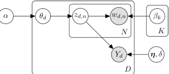
2.2.2 Supervised Latent Dirichlet Allocation
Supervised latent Dirichlet allocation (sLDA, Mcauliffe and Blei [2008]) extends LDA to include a single response variable for each document. Document responses are easily incorporated by using the topic-word distributions (z) to regress onto a response variable. The model also incorporates the regression coefficients in the probabilistic framework. The document responses are linked to their regression coefficients via a generalized linear model (GLM) framework. The leads to the following addition to the generative process of LDA:
• Draw response variable y|Z,η, δ ∼GLM( ¯z,η, δ) where ¯z = N1
N P n=1
zn is the mean of z for each document. The corresponding plate
model is shown in Figure 2.2. There are several features lacking from sLDA that are present in S-GPPF. First, sLDA is a parametric model: the number of topics K must be specified apriori. In practice, the number of topics must be determined using cross-validation as too many topics will lead to several junk topics that provide poor predictive information and do not represent thematic structure. The other major drawback of sLDA is that inference is via an expectation-maximization (EM) approximation to the maximum likelihood. EM provides an inexact estimate of model parameters, and is subject to local maxima.
wd,n Yd zd,n θd α βk η, δ N D K
Figure 2.2: Plate model for supervised latent Dirichlet allocation
2.2.3 Maximum Entropy Discriminant Latent Dirichlet Allocation
Maximum entropy discriminant latent Dirichlet allocation (MedLDA, Zhu et al. [2009]) differs from sLDA in that it optimizes a joint objective function that represents a combination of max-margin learning and a Bayesian topic model. Topics learned in MedLDA not only cluster the data but are learned in an optimal max-margin sense: the latent topics are well suited for use as predictive features. MedLDA provides inference via variational methods, which are detrimental to predictive performance. Additionally, the model has both discriminative and generative components com-bined under a single unified framework, limiting model flexibility. MedLDA is also a parametric model, requiring the number of topics be specified apriori. MedLDA has empirically shown very good performance, and is generally considered state of the art for class prediction in supervised topic modeling.
Further development of MedLDA has led to the so-called Gibbs MedLDA [Zhu et al., 2013]. Gibbs MedLDA employs a Gibbs sampling based inference framework on a completely generative model instead of using variational approximations by using various ideas from Gibbs-based classifiers. However, it does this at the cost of native multiclass classification, requiring a one-versus-all framework to extend binary predictions to the multiclass setting.
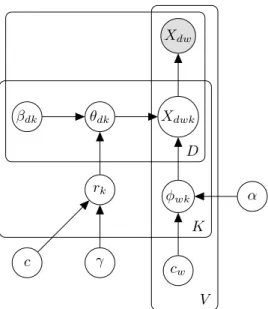
2.2.4 Poisson Count Matrix Factorization
An alternative to an LDA-based topic model is to factorize the corpus (which is represented by a document × word count matrix) using a latent variable model called Poisson factor analysis (PFA, Zhou et al. [2012]). The matrix X ∈ZD×V
+ has
a Poisson likelihood over the observed counts
X ∼Poisson (ΘΦ), (2.1)
where Φ∈RK+×V is the factor loading matrix or dictionary, Θ∈RD+×K is the factor score matrix.
PFA offers two major advantages over classical matrix factorization models that rely on Gaussian observation models [Mnih and Salakhutdinov, 2007]. Gaussian-based factorizations require intricate strategies to mitigate the effects of zeros in settings where zeros represent unobserved entries [Hu et al., 2008]. In contrast, PFA models zeros as the result of finite resources [Gopalan et al., 2013]. This can be easily seen by rewriting the factorization as a two level model: first draw a budget given byxd.,
which is Poisson-distributed according to the likelihood, then allocate the budget onto individual columns following a multinomial distribution (see lemma 2.3.4 for details). This allows PFA to explain zeros as partially due to a lack of resources. The other advantage of PFA is that it need only iterate over non-zero elements. In a latent variable model each element is represented by a summation of latent elements:
xdw= X
k
xdwk
Under a Gaussian likelihood and withxdw= 0, each of the latent values must also be
sampled because xdwk can be both positive and negative. On the other hand, with a
PFA represents a very general framework for factorization of count matrices. A wide variety of algorithms can all be posed as PFA by placing different prior distribu-tions on Φ and Θ. For example, non-negative matrix factorization [Lee and Seung, 2001, Cemgil, 2009], with the objective to minimize the Kullback-Leibler divergence between X and its factorization ΦΘ is PFA solved with maximum likelihood esti-mation. Imposing Dirichlet priors on both the columns of Φ and Θ makes LDA equivalent to PFA in terms of both block Gibbs sampling and variational inference. Placing gamma priors on Φand Θleads to the gamma-Poisson model [Canny, 2004, Titsias, 2008, Gopalan et al., 2014]. This flexibility makes PFA easy to extend to non-parametric factorizations by careful prior selection. A family of negative bino-mial (NB) processes, such as the beta-NB [Zhou et al., 2012, Broderick et al., 2015] and gamma-NB processes [Zhou et al., 2012, Zhou and Carin, 2015], impose different gamma priors onΘ. Marginalizing overΘexplains the latent counts using a gamma-Poisson construction of the negative binomial distribution. For example, the beta-NB process imposes θtk ∼Gamma (rt, pk/(1−pk)), where {pk}1,∞ are the weights of the
countably infinite atoms of the beta process [Hjort, 1990], and the gamma-NB process imposes θtk ∼ Gamma (rk, pt/(1−pt)), where {rk}1,∞ are the weights of the
count-ably infinite atoms of the gamma process. Both the beta- and gamma- NB process PFAs allow the number of latent factors, K, to grow without limits [Hjort, 1990].
As its name implies, S-GPPF uses a gamma process prior to control the number of latent factors. The unsupervised gamma process Poisson factorization [Zhou et al., 2012] has been extended to other problem settings, including dynamic count matrices where columns of the observed count matrix represent observations over time [Acharya et al., 2015] and network modeling where user network information is observed in addition to the count matrix [Zhou, 2015]. A plate model for the gamma process
Xdw Xdwk φwk cw α θdk rk γ c βdk D K V
Figure 2.3: Plate model for Gamma Process Poisson Factorization
Poisson factorization is shown in Figure 2.3.
2.3
Useful Distributions and Results
This section describes several distributions and processes used in the modeling framework of S-GPPF. Several properties are presented in the form of lemmas, the proofs of which can be found in Appendix A.
2.3.1 Gamma Distribution
Throughout this thesis, a random variable x∼Gamma (a, b) has probability den-sity function p(x) = Γ(a1)baxa
−1exp −x b
. This is the shape-scale parameterization of the Gamma distribution with shape a >0 and scaleb >0.
2.3.2 Gamma Process
The gamma process [Ferguson, 1973, Wolpert et al., 2011] G ∼ GaP(c, G0) is a stochastic process whose realizations are random measures: it is a probability
distribution over measures. This is called a completely random measure [King-man, 1967, 1992]. Realizations are drawn from the product space R+ ×Ω. The gamma process is parameterized with concentration parameter c and a finite and continuous base measure G0 over a complete separable metric space Ω, such that G(Ai)∼Gamma(G0(Ai),1/c) are independent gamma random variables for disjoint
partition {Ai}i of Ω. The L´evy measure of the gamma process can be expressed
as ν(drdω) = r−1e−crdrG
0(dω). Since the Poisson intensity ν+ = ν(R+ ×Ω) = ∞ and R
R+×Ωrν(drdω) is finite, following Wolpert et al. [2011], a draw from the gamma
process consists of countably infinite atoms, which can be expressed as: G= ∞ X k=1 rkδωk, (rk, ωk) iid ∼ π(drdω), π(drdω)ν+≡ν(drdω). (2.2) Imposing a gamma process prior on topics, assigns weights corresponding to the atoms of the process to the topics. This leads to the number of active topics being discovered automatically, rather than specified apriori.
2.3.3 Conjugate Prior Distributions
For computational convenience, many of the modeling assumptions are designed using conjugate prior distributions. Some results are presented here in the form of lemmas for ease of deriving the conditional posterior equations in Section 3.2. Lemma 2.3.1. If λ∼Gamma(r,1/c), xi ∼Poisson(miλ), then
λ|{xi} ∼Gamma (r+ P
ixi,1/(c+ P
imi)).
Lemma 2.3.2. If ri ∼ Gamma(ai,1/b) ∀i ∈ {1,2,· · · , K}, b ∼ Gamma(c,1/d), then
b|{ri} ∼Gamma K X i=1 ai+c,1/( K X i=1 ri +d) ! .
Lemma 2.3.3. Ifzi ∼N(µi, σ−1) ∀i∈ {1,2,· · · , K}, σ∼Gamma(a,1/b), thenσ|{zi} ∼
Gamma a+K/2,1/(b+ K X i=1 (zi−µi)2/2 ! .
Lemma 2.3.4. Let xk ∼ Pois(ζk) ∀k, X = PKk=1xk, ζ = PKk=1ζk. If (y1,· · · , yK) ∼
mult(X;ζ1/ζ,· · · , ζK/ζ), then the following holds:
p(x1,· · · , xK) = p(y1,· · · , yK;X).
2.3.4 Negative Binomial Distribution
The negative binomial (NB) distribution m ∼ NB(r, p) has probability mass function Pr(M = m) = Γ(mm!Γ(+rr))pm(1−p)r for m ∈
Z. NB variables can be
con-structed via augmentation into a gamma-Poisson construction as m ∼Pois(λ), λ ∼
Gamma(r, p/(1−p)), where the gamma distribution is parameterized by its shape r and scale p/(1−p). This construction can be extended via the following lemma Lemma 2.3.5. Ifλ ∼Gamma(r,1/c), xi ∼Poisson(miλ), thenx =
P ixi ∼NB(r, p), where p= P imi c+P imi.
The Negative Binomial can also be augmented under a compound Poisson repre-sentation [Zhou et al., 2012, Zhou and Carin, 2012] asm =Pl
t=1ut, ut iid
∼ Log(p), l∼
Pois(−rln(1−p)), where u ∼Log(p) is the logarithmic distribution [Johnson et al., 2005]. The two different constructions are shown graphically in Figure 2.4, and they lead to the following lemma:
Lemma 2.3.6. [Zhou et al., 2012] If m ∼NB(r, p) is represented under its compound Poisson representation, then the conditional posterior of l given m and r has PMF:
Pr(l=j|m, r) = Γ(r)
Γ(m+r)|s(m, j)|r
j, j = 0,1,· · · , m,
where|s(m, j)| are unsigned Stirling numbers of the first kind. We denote this condi-tional posterior as l|m, r∼CRT(m, r), a Chinese restaurant table (CRT) count ran-dom variable, which can be generated vial =Pm
m λ
r
p
(a) Gamma-Poisson Construction
m l
u r
p
(b) Compound Poisson Construction
Figure 2.4: Alternative constructions of the Negative Binomial distribution
This lemma allows leads to the next lemma, which provides closed form sampling of the gamma shape parameter via CRT data augmentation in the gamma-gamma-Poisson framework.
Lemma 2.3.7. If r1 ∼ Gamma(a,1/b), r2 ∼ Gamma(r1,1/d), xi ∼ Poisson(mir2) ∀i, then r1|{xi} ∼ Gamma(a +`,1/(b − log(1 −p))) where ` ∼ CRT(
P i xi, r1), p = P i mi/(d+P i mi) ∀i. 2.3.5 P´olya-Gamma Distribution
A random variable X has a P´olya-Gamma distribution [Polson et al., 2011] with parametersb >0 andc∈R, denotedX ∼P G(b, c), ifX =D 2π12
∞ X k=1
gk
(k−1/2)2+c2/4π2, where gk ∼ Gamma(b,1)’s are independent Gamma random variables, and where
D
= indicates equality in distribution. This leads to the following lemma:
Lemma 2.3.8. [Polson et al., 2013] If ω∼PG(b,0), then exp(ψ)a (1 + exp(ψ))b = 2 −bexp((a−b/2)ψ) Z ∞ 0 exp(−ωψ2/2)p(ω)dω (2.3) ω|ψ ∼PG(b, ψ) (2.4)
P´olya-Gamma random variables are used for augmentation in sampling the state variables that link the count matrix factorization to the document class labels in the S-GPPF model.
2.4
Hinge Loss and Location-mixture of Normals
The support vector machine (SVM) seeks to find a classification function f(x) by solving the following regularized learning problem:
arg min f(x) γ N X n=1 (1−ynf(xn))++R(f(x)), (2.5) where {(xn, yn)}nN=1 is the set of N observation tuples, xn ∈ R is a feature vector
and yn ∈ {−1,1} is the corresponding label for observation n. (1− ynf(xn))+ is the hinge loss, R(f(x)) is a regularization term that controls the complexity off(x), and γ is a tuning parameter controlling the trade-off between error penalization and the complexity of the classification function. The decision boundary is defined as
{x:f(x) = 0} and sign(f(x)) is the decision rule, classifying x as either −1 or 1. Polson et al. [2011] showed that for the linear classifier f(x) = hη,xi, minimizing Eq. (2.5) is equivalent to estimating the mode of the pseudo-posterior of η:
p(η|X,Y, γ)∝ N Y n=1
L(yn|xn,η, γ)p(η), (2.6)
where Y = (y1,· · · , yN) , X = (x1,· · · ,xN),L(yn|xn,η, γ) is the pseudo-likelihood
function, and p(η) is the prior distribution for the vector of coefficientsη. This can be seen by taking the exponential of the negative of Eq. (2.5), where the likelihood is given by the hinge loss and the regularization term is given by the prior on η. Placing a normal distribution prior onη is akin to L2 regularization. Estimating the mode of Eq. (2.6) is equivalent to finding the corresponding minimum of the loss in Eq. (2.5) since they are related under a monotonic transform. Lemma 2.4.1 enables one to solve the optimization problem in Eq. (2.6) using closed form Gibbs sampling updates via data augmentation.
Lemma 2.4.1. [Polson et al., 2011] If u∼N(µ, σ2), one can show that: exp (−2u+) = Z ∞ 0 1 √ 2πλexp −(λ+u) 2 2λ dλ (2.7) where p(λ−1|u)∼IG(kuk−1,1) (2.8) p(u|λ)∼N(µ0, σ02) (2.9) whereµ0 = λ((λµ+−σσ22)), andσ 02 = λσ2
(λ+σ2) andIGdenotes the inverse-gaussian distribution.
2.4.1 Formulation of Multiclass SVM
SVM has also been extended to solve multiclass problems [Weston and Watkins, 1998, Crammer and Singer, 2002, Lee et al., 2004]. Tewari and Bartlett [2007] de-scribes the theoretical consistency of different formulations of multiclass SVMs. S-GPPF uses the formulation of Lee et al. [2004] where the discriminant function for multiclass SVM is defined as fy(x) =hηy,xi,ηy being the weight vector
correspond-ing to the class label y ∈ {1,· · · , M}. The regularized risk minimization problem is given as follows: min η λ 2kηk 2 + D X d=1 X y6=yd hηy,xi+ 1 (M −1) + (2.10) such that M X y=1
hηy,xi = 0 ∀d. This formulation of multiclass SVM is amenable to
tractable inference when the features (i.e. x’s) are latent rather than directly observed as in a hierarchical model: for example, if they represent the assignment of documents to topics in a topic model framework.
Chapter 3
Supervised Gamma Process Poisson Factorization
This chapter describes the supervised gamma process Poisson factorization, which is the main contribution of this thesis. As previously discussed, the novelty of S-GPPF stems from several properties it simultaneously enjoys. First, the model is non-parametric; the number of topics present in a corpus are determined automatically through the use of a gamma process prior on topic weights. Second, the model provides for multiclass classification directly through the use of a multiclass max-margin formulation. Third, the model is fully generative, capturing the relationships between documents, words, topics, and class labels under a completely probabilistic framework. Finally, the model provides for closed form, exact inference through the use of data augmentation and Gibbs sampling. This chapter is structured as follows. Section 3.1 describes the generative process and the latent variables of the model. Section 3.2 details the inference procedure using Gibbs sampling. Section 3.3 describes training the S-GPPF model using documents with known class labels and Section 3.4 details using a trained S-GPPF model to predict unknown class labels.
3.1
Generative Process
Consider a corpus of D documents with a vocabulary of size V. The corpus is partitioned into two sets of documents: those with observed class labels (denoted as the training set) and those without observed class labels (denoted as the testing set). Each document label takes one of M possible values, and the notationyd denotes the
label for the dth document. The document × word count matrix, X, is decomposed as a product of two latent matrices (ΘandΦ) and a topic strength vector (r) under a Poisson likelihood. The generative process is described below, and the corresponding plate model describing the family of distributions of which S-GPPF is a member is shown in Figure 3.1.
For the dth document, sample θ
dk ∼ Gamma (τd,1/exp (−βdk)) ∀k, where τd ∼
Gamma (c0,1/d0),βdk ∼N 0, αdk−1
, and αdk ∼Gamma (g0,1/h0). θdk represents the
affinity of thedth document to thekth topic. Ideally,θ
dk would be used as feature to
predict document class labels. However it is not tractable to do so when using a multi-class max-margin multi-classifier. Instead, βdk is sampled as the per-document features
for classification. From the properties of Gamma distribution, we have E(θdk) = E(τdexp (βdk)) and hence any change inθdk gets reflected in βdk monotonically under
a logarithmic transformation. For thekthtopic, sampleφ
k ∼Dir(ξ) whereφk= (φwk) V
w=1andξis aV−dimensional parameter. Each φwk maps the affinity of word w onto topic k. A Dirichlet prior is
used instead of a hierarchical gamma structure to improve model identifiability. The strength of the kth topic is sampled as r
k ∼ Gamma (γ0/K,1/exp (−ζk)),
where γ0 ∼ Gamma (a0,1/b0), ζk ∼ N 0, νk−1
, and νk ∼ Gamma (u0,1/v0). This places a gamma process prior on the topic strengths, approximating an infinite number of topics with a finite number K; only a small number of topics will be appreciably larger than zero due to the stick-breaking construction of the gamma process. Ideally, therk’s would be used directly as part of the classification weights but as in the case of
θdk this is intractable under a max-margin classifier. Instead, theζk’s are used, which
are monotonically proportional to the rk’s under expectation. Theζk’s represent the
The count corresponding to the dth document and the wth word is sampled as xdw ∼ Poisson P k θdkφwkrk
. Alternatively, due to the property of Poisson distri-bution, one may write xdw =
X k
xdwk, where xdwk ∼ Poisson (θdkφwkrk) ∀k. Each
latent count variable represents the contributions of the kth topic onto the (d, w)th entry in the document ×word matrix.
The class labelyd∈ {1,2,· · · , M}for thedthdocument is calculated using a
multi-class max-margin multi-classifier. From the work of Lee et al. [2004], a pseudo-likelihood of the class label yd is defined as:
q(yd| · · ·) = exp − X y6=yd zyd+ 1 (M −1) + ! (3.1) where zyd ∼ N P k ηykβdkζk, σ−1 , σ ∼ Gamma (s0,1/t0) and M X y=1 zyd = 0. ηy =
(ηyk)Kk=1 is the set of weights corresponding to the yth class and is generated as ηyk ∼
N 0, −k1, k ∼ Gamma (e0,1/f0). ηyk represent the classifier weights for the kth
topic to theyth class label. This is the same formulation of the constrained multiclass SVM as described in Section 2.4.1 with the auxiliary variables {zyd} introduced to
provide closed form inference of the auxiliary variables {βdK} and {ζk} via a data
augmentation scheme.
3.2
Inference
Given the S-GPPF sampling model and a corpus, the main problem is posterior inference: finding the distribution of the model parameters given the observed data. Since S-GPPF seeks to also predict test set class labels, the unobserved class labels are also considered as unknown parameters. One method for estimating the poste-rior is through the use of Markov chain Monte Carlo Methods (MCMC, Hoff [2009],
Xdw Xdwk φwk θdk τd βdk αdk rk ζk νk γ0 ηyk k zyd σ yd ξw a0 b0 c0 d0 e0 f0 g0 h0 t0 s0 v0 u0 D K V M
Gamerman and Lopes [2006]). MCMC methods describe Markov chains that are easy to sample from and whose invariant distributions are the target posterior. Then the samples from the Markov chain are also distributed according to the posterior, and the distribution can be estimated via Monte Carlo integration. For a Markov chain to converge to its invariant distribution regardless of its initialization, it must be irreducible, invariant, and aperiodic [Cosma and Evers, 2010].
Hierarchical Bayesian models such as S-GPPF naturally lend themselves to Gibbs sampling [Cosma and Evers, 2010, Hoff, 2009, Gamerman and Lopes, 2006]. In Gibbs sampling, the conditional posterior distributions for each parameter are sampled pro-gressively one by one (there are other Gibbs sampling schemes, such as random scan but systematic scanning is considered here for simplicity). Parameters are drawn using the most recent samples of all of the other parameters. It has been shown that Gibbs sampling schemes are invariant [Cosma and Evers, 2010], so to show that a Gibbs sampling scheme is valid for posterior inference it must be shown to be aperi-odic and irreducible.
The proposed Gibbs sampling scheme for S-GPPF is easily shown to have both of these properties. With the exception of the latent count variables (xdwk), all of
the parameters are drawn either from gamma or normal distributions (excluding the augmented variables, since they are marginalized out). As such, each variable has positive probability mass on its entire state-space (eitherR,R+, orRK). This means that regardless of the current state of the chain, there is some positive (although it may be very small) probability to move to any other valid state. Therefore, the Gibbs sampling scheme forms an irreducible Markov chain. Furthermore, since the entire state space has positive probability mass, there is positive mass on staying in the same state. This implies that the chain is also aperiodic and therefore the Gibbs
sampling scheme is valid for posterior inference.
Enumerated below are the conditional posterior distributions for each of the model parameters. Full derivations of the sampling equations are provided in Appendix B. Sampling of (xdwk)Kk=1 (xdwk)Kk=1| · · · ∼mult rkθdkφwk K X k=1 rkθdkφwk K k=1 ;xdw (3.2) Sampling of θdk θdk| · · · ∼Gamma (τd+xd.k,1/(exp (−βdk) +rk)) (3.3) Sampling of τd ldk| · · · ∼CRT (xd.k, τd) (3.4) τd| · · · ∼Gamma c0+ X k ldk,1/(d0− X k log(1−pdk)) ! , (3.5) where pdk = exp(−βrk dk)+rk. Sampling of φk φk| · · · ∼Dir (ξ1+x.1k,· · · , ξV +x.V k) (3.6)
Sampling of rk rk| · · · ∼Gamma (γ0/K+x..k,1/(exp (−ζk) +θ.k)) (3.7) Sampling of γ0 lk| · · · ∼CRT (x..k, γ0/K) (3.8) γ0| · · · ∼Gamma a0+ X k lk,1/(b0− 1 K X k log(1−pk)) ! , (3.9) where pk= exp(−θζ.kk)+θ.k. Sampling of σ σ| · · · ∼Gamma s0+ M D 2 ,1/t 0 0 , (3.10) where t00 = t0+ X y,d (zyd− P k ηykβdkζk)2 2 . Sampling of k k| · · · ∼Gamma e0+ M 2 ,1/ X y η2 yk 2 +f0 !! (3.11) Sampling of νk νk| · · · ∼Gamma u0+ 1 2,1/ ζk2 2 +v0 (3.12)
Sampling of αdk αdk| · · · ∼Gamma g0+ 1 2,1/ β2 dk 2 +h0 (3.13) Sampling of zyd Since M P y=1
zyd = 0, we need only sample {zyd}y6=yd for each document d and assign
zydd=− P y6=yd zyd. Then for y6=yd: γyd| · · · ∼IG zyd+M1−1 2 −1 ,1 (3.14) zyd| · · · ∼N µ0, σ02 (3.15) where σ02 = γyd γydσ+1/4 and µ 0 =σ02 σP k βdkηykζk− 4γ 1 yd(M−1) − 1 2 , and IGis used to denote the inverse-Gaussian distribution.
Sampling of ηy ηy| · · · ∼N(µy,Σy), (3.16) where Σ−1 y = α1IK +σ(ζIK) P d (β0dβd) (ζIK) and µy =Σy σηy(ζIK) P d zydβd0 Sampling of βd ωdk| · · · ∼PG(xd.k+τd, βdk+ log(rk)) (3.17) βd| · · · ∼N(µd,Σd), (3.18)
where Σ−d1 = (αdIK) + (ωdIK) +σ(ζIK)P y ηy0ηy (ζIK) , µd= σP y [zydηy] (ζIK)−ωd(log(r)IK) + ν2d Σd, and νd={xd.k−τd}Kk=1. Sampling of ζ ωk| · · · ∼PG(x..k+γ0/K,log(θ.k) +ζk) (3.19) ζ| · · · ∼N(µ,Σ), (3.20) where Σ−1 = " (α2IK) + (ωIK) +σP y,d (βdIK)η0yηy(βdIK) # , µ= " σP y,d zydηy(βdIK)−log(θ)(ωIK) +λ/2 # Σ,λ={x..k−γ0/K}Kk=1, and θ ={θ.k}Kk=1.
3.3
Training Phase
In the training phase, the document class labels are observed and all model vari-ables are sampled in a Gibbs sampling scheme. The implementation used in this thesis forms parameter estimates after the training phase by computing the sample average as a Monte Carlo approximation of the posterior mean. This provides a point estimate for parameters that can be easily used for sampling in the test phase.
It is worth noting that since topics are related to both observed counts and class labels only through inner products, the resulting posterior distribution is not identi-fiable: the exact index, k, for a specific topic will vary between runs of the Markov chain. This has important ramifications for propagating multiple samples instead of single point estimates of parameters for the test phase. It is certainly possible to run separate chains for each sample, but care must be taken when concatenating the
samples: results should only be combined at the level of the observed data, i.e. it is invalid to combine the samples of θdk from multiple chains as draws from the same
posterior but it is valid to combine P k
θdkrkφwk across chains as all being drawn from
the same posterior.
The experiments presented in Chapter 4 use only point estimates of the posterior mean from the training phase. This makes the implementation simpler and eases the computational burden since only a single chain is run in test phase, but it is a simplification. In fact, using a point estimate gives up some of the advantage gained by using a fully generative framework with exact inference as an estimate of the full posterior distribution is no longer available. Incorporating better estimates between training and test phases provides an opportunity for improvement upon the work presented in this thesis.
3.4
Test Phase
The goal in the training phase it to estimate the model parameters that are not specific to any document. The test phase then uses these estimates to sample the posterior of the document specific parameters and uses the result to predict the un-known class labels. In test phase, the posterior mean estimates from training for all of the parameters that not document specific are held fixed. Gibbs sampling is then run on only those variables that are document specific. This means that for each test document d, only {θdk}Kk=1,{xdwk}kK,V=1,w=1, βd, and {αdk}Kk=1 are sampled. Since the class labels are unknown, βd is sampled without the influence of zyd, σ, and yd. To
estimate the class labels,zyd is estimated by its mean, given byP k
βdkηykζk. The class
Chapter 4
Experiment Analysis
This section describes using the S-GPPF model on two different datasets: a syn-thetic dataset used to explore and visualize the latent variables of the model and a corpus of abstracts from several conferences to compare the performance of S-GPPF against competing supervised topic models. S-GPPF is shown to have state-of-the-art levels of performance for classification of document labels.
4.1
Factorization of Synthetic Data
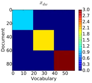
This section considers a synthetic corpus to gain intuition into the model parame-ters. The data has 90 documents and 60 words arranged in a block diagonal structure. The upper third of the block diagonal are assigned a count value of one, the middle third are assigned a count value of two, and the final third block diagonal are assigned a value of three. All other values in the document × word matrix are set to zero. Accordingly, the first third of the documents are assigned a class label of one, the second third are assigned a class label of two, and the final third are assigned a class label of three. The document × word matrix and class labels are shown in Fig 4.1. Sampling is run for 1,000 iterations, with the first 500 discarded and the last 500 averaged to generate point estimates of the posterior mean for the parameters. These estimates are what is displayed throughout this section.
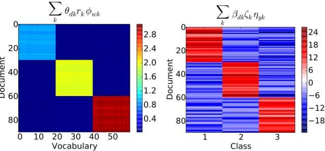
The S-GPPF accurately models the synthetic data. To illustrate this, the original document × word count matrix and document class labels are estimated from the
0 10 20 30 40 50
Vocabulary
0
20
40
60
80
Document
x
dw
0.0
0.3
0.6
0.9
1.2
1.5
1.8
2.1
2.4
2.7
3.0
(a) Document×Vocabulary count matrix.
0
20
40
60
80
Document
y
d
0.0
0.3
0.6
0.9
1.2
1.5
1.8
2.1
2.4
2.7
3.0
(b) Document class labels.
Figure 4.1: Synthetic block diagonal data
model parameter estimates. Since the data is assumed to be drawn from a Poisson likelihood, the count matrix is estimated as ˆxdw =
K P k=1
θdkrkφwk. Similarly, the zyd
parameters are estimated by their mean, ˆzyd = P
k
βdkζkηyk. The class labels can then
be estimated by Eq. (3.1). These parameter estimates are shown in Fig 4.2.
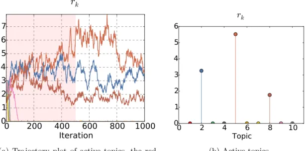
The next thing to evaluate is whether the Markov chain has converged to the stationary distribution and if the non-parametric process is working as expected. An ad-hoc method for assessing the convergence of Gibbs sampling is to examine trajectory plots of parameter samples. Such trajectory plots are generated for the strength of the topics, given byrk in Figure 4.3. The red region on the plot highlights
the “burn-in” iterations. The trajectory plots are indicative of a chain which has reached its invariant distribution. From the clearly defined block diagonal structure in the input data, three distinct topics should emerge from the data. The gamma process prior on rk allows for the automatic discovery of the number of topics. In
0 10 20 30 40 50
Vocabulary
0
20
40
60
80
Document
Xk
θ
dk
r
k
φ
wk
0.4
0.8
1.2
1.6
2.0
2.4
2.8
(a) Estimate of Document × Vocabulary count matrix from model parameters.
1
2
3
Class
0
20
40
60
80
Document
Xk
β
dk
ζ
k
η
yk
18
12
6
0
6
12
18
24
(b) Estimate ofz matrix from the model pa-rameters.
Figure 4.2: Reconstructed block diagonal X and z matrices
(see Figure 4.3) assigns significant weight to only three topics, which is the desired behavior in non-parametric modeling. A parametric model (such as LDA) assigns weights for all ten topics.
To further explore and understand the latent topic space of S-GPPF, it is useful to examine the mappings from documents and words to latent topics. Given the block diagonal input structure, each third of documents should map onto its own topic. The affinity between documentdand topick is computed asθdk
√
rk. This quantity can be
thought as the degree to which the content of document d is from topic k. Likewise, each third of the vocabulary should map onto a single topic, and that topic should be the same as the corresponding third of documents (due to the block diagonal input structure). The affinity between word w and topic k is computed as φwk
√
rk. This
quantity gives the relative weighting for a word w onto the topics. The document-and word- topic affinities are shown in Figure 4.4, document-and have the expected structure.
0
200 400 600 800 1000
Iteration
0
1
2
3
4
5
6
7
r
k
(a) Trajectory plot of active topics, the red highlight indicates burn-in iterations
0
2
4
6
8
10
Topic
0
1
2
3
4
5
6
r
k (b) Active topicsFigure 4.3: Active topics in synthetic data
Note that the product of these matrices leads to the estimate for xdw, as shown in
Figure 4.2.
Also of value to explore are the higher level document and class mappings that are used for class label prediction. Recall that using the document-to-topic map-pings given byθdk
√
rkdirectly as the classification feature matrix is intractable under
the multiclass max-margin formulation used in S-GPPF. Instead, βdk and ζk are
in-troduced, which are logarithmically proportional under expectation to θdk and rk,
respectively. Ideally, the higher level document-to-topic affinities given by βdk should
have similar structure as θdk. The classification weights to assign class label y from
topic topic k is given by ηykζk. Under the block-diagonal structure of the data, the
class label of each third of documents should map onto the same latent topic as its corresponding documents. These quantities are shown in Figure 4.5, and have the desired structure. Note that the product of these matrices leads to the estimate for
0
2
4
6
8
Topic
0
20
40
60
80
Document
θ
dk
pr
k
3
6
9
12
15
18
21
24
(a) Document-to-topic affinity
0
2
4
6
8
Topic
0
10
20
30
40
50
Vocabulary
φ
wkpr
k0.015
0.030
0.045
0.060
0.075
0.090
0.105
(b) Vocabulary-to-topic affinityFigure 4.4: Document- and word- topic affinities in synthetic data
zyd, as shown in Figure 4.2.
4.2
ACM Conference Abstracts Classification
The ACM conference abstracts text corpus described by Acharya et al. [2013] con-sists of abstracts collected from four data mining related conferences and two VLSI conferences. The data mining conferences are Knowledge Discovery and Data Mining (KDD), the International Conference on Machine Learning (ICML), the Special Inter-est Group on Information Retrieval (SIGIR), and the International World Wide Web conference (WWW). The two VLSI conferences are the International Symposium on Physical Design (ISPD), and the Design Automation Conference (DAC). A total of 5,755 abstracts were collected. The documents in this dataset are abstracts and the class labels are the conferences in which each abstract appeared.
The abstracts are preprocessed as follows: each abstract is converted to a count vector under a bag-of-words assumption. Bag-of-words assumes that the specific
0
2
4
6
8
Topic
0
20
40
60
80
Document
β
dk
4
3
2
1
0
1
2
3
(a) Higher level document-to-topic affinity
0
2
4
6
8
Topic
1
2
3
Class
η
yk
ζ
k
2.4
1.6
0.8
0.0
0.8
1.6
2.4
3.2
4.0
(b) Class-to-topic affinityFigure 4.5: Class regression parameters in synthetic data
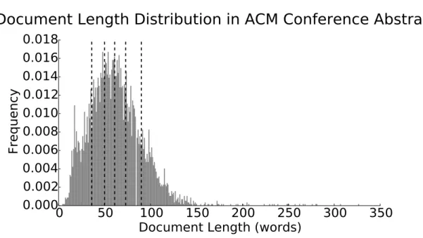
ordering of words within a text document is unimportant (this is not really the case: consider any paragraph in this document as an example). Hence each document is represented as a “bag” of the words found in the document. Raw text is tokenized using the Natural Language Tool Kit (NLTK, Loper and Bird [2002]) word tokenizer with punctuation and numeric words stripped from the resulting tokens. Tokens are stemmed using a Porter stemmer [Porter, 2001]. The set of English stop words provided by NLTK are removed from the resulting tokens. Additionally, rare corpus words (words that appear in less than 1% of all documents) and corpus specific stop words (words that appear in more than 50% of all documents) are also removed. After preprocessing, the vocabulary size is 971 words. A histogram of document lengths (in words) is provided in Figure 4.6. The black vertical lines indicate the edges of bins used to compute classification accuracy vs. document length. The document frequency of words and the number of document per length bin are shown in Figure 4.7.
0
50
100 150 200 250 300 350
Document Length (words)
0.000
0.002
0.004
0.006
0.008
0.010
0.012
0.014
0.016
0.018
Frequency
Document Length Distribution in ACM Conference Abstracts
Figure 4.6: Distribution of abstract lengths (in words) of ACM conference data. Black lines denote the bins used for computing classification accuracy vs doc length (see Figure 4.9)
10 % 20 % 30 % 40 %
Document Frequency
0
50
100
150
200
250
300
Number of Words
Document Frequencies for
ACM Conference Vocabulary
(a) Document frequencies of words in ACM conference dataset vocabulary after prepro-cessing.
[0-36][36-50][50-61][61-73][73-90][90-350]
Bin Edges (words)
Number of Documents
1013 1012
925 950 955 900
Number of Documents Per Bin
(b) Number of documents assigned to each document length bin.
The following models are also run on the ACM conference abstracts dataset with identical preprocessing to compare against S-GPPF. All model parameters were se-lected using a standard 10-fold cross validation on the entire dataset.
• Maximum entropy discrimination latent Dirichlet allocation (MedLDA, Zhu et al. [2009]). Model parameters are the number of topics, K = 50, and the max-margin penalty factor,C = 30. This model is intended as a strong baseline as it jointly models both the class labels and count matrix, and is generally considered state-of-the-art in supervised topic modeling.
• Latent Dirichlet allocation [Blei et al., 2003] with support vector machine (LDA + SVM). LDA is fit on the entire dataset, and the resulting document-topic matrix (the θ parameter from LDA) is used as the feature matrix for a linear support vector classifier. Model parameters are the number of topics, K = 50, and the standard linear SVM tuning parameters with margin penaltyC = 1.0. This model is intended as a weak baseline, as topics and class labels are learned in a disjoint manner.
Tests are run as follows. Twenty five independent splits of the data into equal test and train sets are generated, maintaining class proportions to be the same as in the whole dataset. Results are aggregated across independent splits, computing the mean and standard deviation (the standard deviation is represented in performance plots as error bars). Within this framework, accuracy is compared against two different variables: amount of training data and document length. The model is sampled for two thousand burnin and two thousand collection iterations for each independent run of the model.
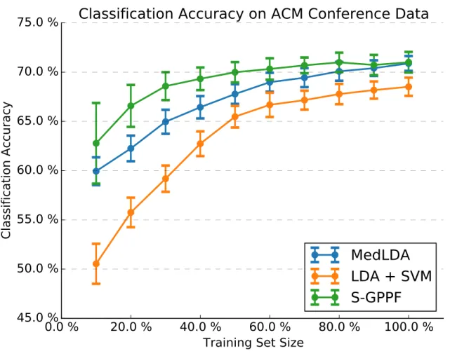
The first test compares classification accuracy vs. the amount of training data. For each train/test split, only a portion of the training data is available to the mod-els. The training data is subsampled to maintain relative class proportions in 10% increments up to 100% of the training data. The results of this test are shown in Fig-ure 4.8. Since S-GPPF is a fully generative model, it outperforms the state of the art model, MedLDA, by a large margin when there is limited training data available. By using fully probabilistic priors, S-GPPF better generalizes to unseen data than dis-criminative models. The LDA + SVM performs worse than S-GPPF and MedLDA, which both jointly learn the topics and labels. This is exaggerated for small amounts of training data since the topics learned in the disjoint model are not well suited to the classification task.
The second test compares classification accuracy vs. document length. All of the training data is available in these tests. The documents are binned in to equal volume bins (see Figure 4.6 for the bin placement and Figure 4.7 for the bin volume). Classification accuracy is then computed for each of the bins. The results of the test are shown in Figure 4.9. These plots show that S-GPPF uniformly outperforms competing supervised topic models for widely varying document lengths, a useful property for modeling the long tail often found in real-world data [Gopalan et al., 2013].
The topics learned in S-GPPF are easily interpreted. To visualize this, a single run of S-GPPF is considered using all of the available training data. For each conference, the document-to-topic weights (θdk
√
rk) are summed along the document axis and the
topic with the greatest weight for each conference is considered. Each topic can be viewed as a distribution over words, given by φwk. The top ten words (by weight) for
0.0 %
20.0 %
40.0 %
60.0 %
80.0 %
100.0 %
Training Set Size
45.0 %
50.0 %
55.0 %
60.0 %
65.0 %
70.0 %
75.0 %
Classification Accuracy
Classification Accuracy on ACM Conference Data
MedLDA
LDA + SVM
S-GPPF
Figure 4.8: ACM conference abstracts classification accuracy vs. percent of training data observed
0
50
100
150
200
250
Document Length
55.0 %
60.0 %
65.0 %
70.0 %
75.0 %
80.0 %
85.0 %
90.0 %
Classification Accuracy
Classification Accuracy on ACM Conference Data
MedLDA
LDA + SVM
S-GPPF
Figure 4.9: ACM conference abstracts classification accuracy vs. document length in words
KDD ICML SIGIR WWW ISPD DAC
deal algorithm dynamic server plan system
mixture outperform return weight router device
algorithm minimum query appropriate device appropriate
people propose test provide algorithm throughput
growth embed baseline system chain life
propose baseline insert difficulty baseline simulate approximate gather minimum utility throughput methodology
set retrieval reliable deal retrieval period
differentiable configure period baseline outperform arising
minimum set approximate internet worst process
recall solve independent procedure learn technology decision architecture propose determine busy solution
retrieval context textual ir view hidden
strong approximate latter supply intelligent partial Table 4.1: Top topic for each conference
(KDD, ICML, SIGIR, and WWW) feature words related to data mining: minimum, query, approximate, etc. The VLSI conferences (ISPD and DAC) prominently feature words related to the VLSI field: router, throughput, device, etc. This indicates that the Poisson factorization captures the low dimensional topic space known to exist in the data.
Chapter 5
Conclusion
S-GPPF represents a novel supervised topic model due to its unique properties. S-GPPF addresses the supervised topic modeling in a fully probabilistic framework. It directly models multiclass document labels and automatically selects the number of latent topics present in a corpus. Furthermore, S-GPPF provides for exact infer-ence by using several data augmentation techniques for closed form Gibbs sampling updates. S-GPPF is shown to provide state-of-the-art levels of performance, simul-taneously learning clearly interpretable features and document class labels. Because of its fully probabilistic framework, S-GPPF gains further advantage over competing models when the amount of training data available is limited.
This chapter is structured as follows. Section 5.1 provides suggestions on imple-menting and running S-GPPF in practical applications. Section 5.2 concludes this thesis with a discussion of further avenues of research and provides final thoughts.
5.1
Practical Suggestions
S-GPPF is a good choice for document classification when the resulting classifier should use clearly interpretable features in its decisions. The latent topic representa-tion makes the S-GPPF model easy to interpret, as documents and class labels are represented as mixtures of topics which are in turn mixtures of words. The fully gen-erative nature of S-GPPF makes the class-decision rules easy to understand as they are given by probability distributions. S-GPPF also gains clear advantage when the
number of topics present in a corpus is not easily discernible or known apriori: extra topics are automatically pulled to zero to avoid junk topics. This means that S-GPPF can be used to estimate the number of clusters in a labeled corpus. Additionally, S-GPPF gains substantial computational benefits by not requiring a cross-validation over the number of topics.
The implementation of S-GPPF used in this thesis leads to several suggestions regarding efficient computation and numeric stability in practice. This implemen-tation makes use of the Armadillo C++ library for linear algebra [Sanderson, 2015] and the GNU Scientific Library [Galassi et al., 2010] for random number generation. The conditional posterior sampling requires the inversion ofK×K precision matrices for multivariate normal sampling. Recognizing that precision matrices are positive semi-definite allows for more stable and faster methods of inversion such as through the use of the Cholesky decomposition, which is provided by the Armadillo library.
Samplers for several of the distributions found in the conditional posterior updates are not readily available in common libraries: namely the Chinese restaurant table count, P´olya-Gamma, and inverse-Gaussian random variables. The Chinese restau-rant table can be implemented as a sum of Bernoulli draws with varying parameters [Zhou et al., 2012] and inverse-Gaussian sampling can be implemented using a Gaus-sian sampler [Michael et al., 1976]. Polson et al. [2013] describe an efficient sampler for P´olya-Gamma random variables, but it requires integer valued parameters. S-GPPF makes use of P´olya-Gamma random variables with real-valued parameters, requiring a truncation of an infinite sum of gamma distributed random variables. Such a sum works wells for most parameter values, but becomes unstable for small floating point values of parameters. The parameter values required for S-GPPF are very small due to the sparsity in latent topics. The implementation used in this thesis corrects for
this floating point bias by scaling the result of the P´olya-Gamma sampler to ensure that the first moment of the resulting samples maintains the expected value.
Other variables in the model are subject to floating point errors when they become sufficiently small. Specifically,rkand θdk (since they are sparse in topic space and are
used under a logarithmic transform in the sampling of other variables) and αdk, k,
andνk(since they represent precisions). Since the values need only be small compared
to the active topic values, a minimum value clamp can be used to prevent numerical instabilities. The implementation used here clamps these variables to greater than 10−10.
5.2
Discussion and Future Work
There is room for improvement in the classification performance of S-GPPF due to the multi-class max-margin formulation used. The formulation requires the introduc-tion of the latentzyd random variables, which add Gaussian noise to the classification
features. The zyd’s are needed due to the sum-to-zero constraint of Eq. (2.5). This
constraint makes it intractable to directly linkη,β, andζ to the class labels. Adopt-ing a different multi-class max-margin formulation or data augmentation strategy that does not require the introduction of z should lead to an increase in classifier performance. Additionally, the current formulation does not fit intercepts. Adding an intercept term to the learned parameters could also boost classifier performance.
The multi-class nature of S-GPPF can be extended to a multi-task setting. The latent variables are already formulated in a multi-task framework: different class labels serve as an inductive bias for inferring document labels. The existing classifier structure suggests easy extensions to problems where a vector of binary labels are observed for each document rather than a single multi-class response variable. In such
a problem, a document may belong to multiple classes: for instance, a movie may belong to multiple genres. The framework can also be extended to the active learning setting similar to Acharya et al. [2013]. In the active learning setting, classification labels are very expensive to obtain. The modeling process formulates queries of the training examples for which class labels would be the most informative in modeling. S-GPPF fits neatly into a group of several models which extend non-parametric PFA to problems in which information in addition to the count matrix is observed. In S-GPPF, document class labels are also observed. Acharya et al. [2015] extends PFA to modeling count matrices when the columns are temporally related. Zhou [2015] jointly models count matrices along with network side information. There is potential to unify these modeling extensions under a single, broad non-parametric PFA framework. Such a framework could jointly model count matrices with the side information available on a case-by-case basis.
This thesis developed and presented the supervised gamma process Poisson fac-torization model. S-GPPF represents a novel supervised topic model; it is fully gen-erative and nonparametric, allows for multi-class classification, and provides for exact inference via Gibbs sampling. S-GPPF is shown to outperform MedLDA and other competing topic models for classification. S-GPPF fits neatly into a framework of ex-tending the broad class of algorithms that can be unified under Poisson factorization to including additional side information.
Appendix A
Proofs of Lemmas
Proof of lemma 2.3.1. The proof follows directly from application of Bayes’ rule
p(λ|{xi})∝p(λ|r, c) Y i p(xi|mi, λ) ∝λr−1exp (−λc)Y i λxiexp (−m iλ) =λr+ P i xi−1 exp −λ c+X i mi !! =⇒ λ|{xi} ∼Gamma r+ X i xi,1/ c+ X i mi !!
Proof of lemma 2.3.2. This lemma follows directly from application of Bayes’ rule
p(b|{ri})∝p(b|c, d) Y i p(ri|ai, b) = Gamma (b;c,1/d)Y i Gamma (ri;ai,1/b) ∝bc−1exp (−bd)Y i baiexp (−r ib) =bc+ P i ai−1 exp −b d+X i ri !! =⇒ b|{ri} ∼Gamma c+ X i ai,1/ d+ X i ri !!
Proof of lemma 2.3.3. This lemma follows directly from application of Bayes’ rule p(σ|{zi})∝p(σ|a, b) K Y i=1 p(zi|µi, σ) = Gamma (σ;a,1/b) K Y i=1 N zi;µi, σ−1 ∝σa−1exp (−σb) K Y i=1 σ1/2exp −σ(zi−µi) 2 2 ! =σa+K/2−1exp −σ b+ K X i=1 (zi−µi)2 2 !! =⇒ σ|{zi} ∼Gamma a+K/2,1/ b+ K X i=1 (zi−µi)2 2 !!
Proof of lemma 2.3.4. The joint distribution for {yk}Kk=1 is given as p(y1,· · · , yK;X) =X! K Y k=1 (ζi/ζ)yk yk! = X! ζX K Y k=1 ζyk k yk! ∝1 " K X k=1 yi =X # K Y k=1 ζyk k yk!
which has the same form as p(x1,· · · , xK) since K P k=1
xk =X by construction.
Proof of lemma 2.3.5. Since a summation of Poisson random variables is also a Pois-son, x ∼ Poisson λP i mi
distribution of x: p(x) = ∞ Z 0 Gamma (λ;r,1/c) Poisson x;λX i mi ! dλ = ∞ Z 0 λr−1exp (−λc) crΓ(r) λP i mi x x! exp −λ X i mi ! dλ = P i mi x cr x!Γ(r) ∞ Z 0 λr+x−1exp −λ c+X i mi !! dλ = P i mi x cr x!Γ(r) Γ(r+x) c+P i mi r+x = Γ(r+x) x!Γ(r) P i mi c+P i mi x 1− P i mi c+P i mi r =⇒ x∼NB r, P i mi c+P i mi
Proof of lemma 2.3.6. The derivation of this lemma is found in Zhou et al. [2012]. Proof of lemma 2.3.7. Since the summation of Poisson random variables is also Pois-son, x =P i xi ∼Poisson r2 P i mi
. From lemma 2.3.5, this implies x∼ NB(r1, p) where p = P i mi d+P i
mi. Then from the compound Poisson construction of the Negative
Binomial, l ∼ Poisson (−r1log(1−p)). From lemma 2.3.6, l|x, r1 ∼ CRT(x, r1). Fi-nally, by the gamma-Poisson conjugacy (lemma 2.3.1),
Appendix B
Conditional Posterior Derivations
Sampling of (xdwk)Kk=1
The conditional posterior of (xdwk)Kk=1 follows directly from the multinomial-Poisson distribution equivalence lemma 2.3.4.
p(xdw1,· · · , xdwK| · · ·)∝ Y k p(xdwk|rk, θdk, φwk) =Y k Poisson (xdwk;rkθdkθdk) xdw= X k xdwk (xdwk)Kk=1| · · · ∼mult rkθdkφwk K X k=1 rkθdkφwk K k=1 ;xdw (B.1) Sampling of θdk
The conditional posterior of θdk follows directly from the gamma-Poisson conjugacy
lemma 2.3.1.
p(θdk| · · ·)∝p(θdk|βdk, τd)p(xd.k|rk, θdk)
= Gamma (θdk;τd,exp (βdk)) Poisson (xd.k;rkθdk)
Sampling of τd
The conditional posterior of τd follows by repeated application of the CRT
aug-mentation lemma 2.3.7. Introduce ldk ∼ Poisson (−τdln (1−pdk)) where pdk =
P k
rk
exp(−βdk)+rk. The posterior is then found by application of the gamma-Poisson
conju-gacy lemma 2.3.1. Then
ldk| · · · ∼CRT (xd.k, τd) (B.3) τd| · · · ∼Gamma c0+ X k ldk,1/(d0− X k log(1−pdk)) ! (B.4) Sampling of φk p(φk| · · ·)∝p(φk|ξ) Y p(x.wk|rk, θ.k, φwk) φk| ∼Dir (ξ1+x.1k,· · · , ξV +x.V k) (B.5) Sampling of rk
The conditional posterior of rk follows directly from the gamma-Poisson conjugacy
lemma 2.3.1.
p(rk| · · ·)∝p(rk|γ0, ζk)p(x..k|rk, θ.k)
= Gamma (rk;γ0/K,exp (ζk)) Poisson (x..k;rkθ.k)
rk| ∼Gamma (γ0/K+x..k,1/(exp (−ζk) +θ.k)) (B.6)
Sampling of γ0
The conditional posterior of γ0 follows by repeated application of the CRT aug-mentation lemma 2.3.7. Introduce lk ∼ Poisson (−γ0/Kln (1−pk)) where pk =