Digital twin using multivariate prediction

Digital Twin using Multivariate Prediction

Jere Puolakanaho

2380155

Research Unit of Mathematical Sciences

University of Oulu

Abstract

Digital Twin is a digital replica of physical assets, processes and systems that can be used for various purposes. Virtual model is constructed from the corresponding physical model and these two are then connected by generating real time data using sensors. Resent advances in technology have enabled this, because they have made digital environments cost-efficient. The goal is to simulate the real world with minimal physical resources using machine learning, multivariate analysis and other mathematical techniques. Optimally no physical resources go to waste in testing and development.

Runtime validation means monitoring and validating a running system with both digital and physical models. Simulated (digital) model parameters are used in the physical model and then the simulated model is updated with new data from the physical model. Simulated model gains more and more data over time becoming more accurate.

This thesis studies the applicability of mathematical models as a prediction tool to predict and validate systems behaviour as a part of simulation. And further, be used in analysis in a digital twin model.

Keywords: Digital Twin, multivariate analysis, prediction, runtime validation

Tiivistelm¨

a

Digitaalinen kaksonen on digitaalinen kopio fyysisist¨a voimavaroista, prosesseista ja systeemeist¨a, jota voidaan k¨aytt¨a¨a moniin tarkoituksiin. Virtuaalinen malli rakennetaan vastaavasta fyysisest¨a mallista ja n¨am¨a yhdistet¨a¨an toisiinsa luomalla reaaliaikaista dataa sensoreilla. Viimeaikaiset kehitykset teknologiassa ovat mahdollistaneet t¨am¨an tekem¨all¨a digitaalisista ymp¨arist¨oist¨a kustannustehokkaita. Teht¨av¨an¨a on simuloida oikeaa maailmaa minimaalisilla fyysisill¨a resursseilla k¨aytt¨aen koneoppimista, monimuuttuja-analyysi¨a ja muita matemaattisia tekniikoita. Parhaimmillaan fyysisi¨a resursseja ei menisi hukkaan testauksessa ja kehityksess¨a.

Ajonaikainen validointi tarkoittaa toimivan systeemin tarkkailua ja validointia fyysisen ja digitaalisen mallin avulla. Simuloidun (digitaalisen) mallin arvoja k¨aytet¨a¨an fyysisess¨a mallissa ja simuloitua mallia p¨aivitet¨a¨an uudella datalla fyysisen mallin tulosten perusteella. Simuloitu malli saa yh¨a enemm¨an dataa ajan saatossa ja t¨at¨a my¨ot¨a paranee.

T¨am¨a tutkielma tutkii matemaattisten mallien k¨aytett¨avyytt¨a ennustukseen ja systeemin validointiin sek¨a simulaatiossa ett¨a digitaalisen kaksosen analyysiss¨a.

Avainsanat: Digitaalinen kaksonen, monimuuttuja-analyysi, ennustaminen, ajonaikainen validointi

Foreword

I want to thank Nokia Solutions and Networks for providing me this opportunity to do my master’s thesis for their company. This process of making the thesis was a fascinating and educational journey. I have learned a lot about Nokia as a company and community. New topics that came through this journey have kindled my interest to continue on this career/profession.

From the Nokia Solutions and Networks, I want to especially thank my thesis supervisor Mr. Pekka Tuuttila, and Mrs. Kirsti Simula. Your technical guidance and feedback helped me a lot during this process. Thank you for keeping me motivated.

From the University of Oulu, I want to thank my principal supervisor docent Erkki Laitinen for guiding me in my studies and through this process. I also want to thank Leena Ruha, PhD, for being the second examiner of my thesis. I want to thank the University of Oulu and the Research Unit of Mathematical Sciences for offering magnificent education during these five years.

This master thesis work has received funding from the Electronic Component Systems for European Leadership Joint Undertaking under grant agreement No 737494. This Joint Undertaking receives support from the European Union’s Horizon 2020 research and innovation programme and Sweden, France, Spain, Italy, Finland, Czech Republic.

Abbreviations and symbols

SSres Sum of Squares of Residuals

SStot Total Sum of Squares

ALD Analysis-Led Design ANN Artificial Neural Network DTA Digital Twin Aggregate DTE Digital Twin Environment DTI Digital Twin Instance DTP Digital Twin Prototype

LS-SVM Least-Squares Support-Vector Regression MVA Multivariate Analysis

NIPALS Non-linear Iterative Partial Least Squares PCA Principle Component Analysis

PCR Principal Component Regression PLM Product Lifecycle Management

PLS Partial Least Squares or Projection to Latent Structures PRESS Predictive Error Sum of Squares

RDA Redundancy Analysis

RMSEP Root Mean Squared Error of Prediction SVD Singular Value Decomposition

SVR Support-Vector Regression

VIP Variable Importance in Projection Symbol

λ Eigenvalue

B Regression coefficient matrix

C Loading ofY

Cxy Covariance matrix ofX and Y

E Error matrix

H Score ofY

i Index number

j Index number

P Loading ofX

Pw(x) The projection of a vector x onto a vector w

Q2 _{Goodness of prediction}

R2 Goodness of fit

T Score ofX

X Input matrix

xij Element of input matrix

Y Output matrix

Contents

Abstract 1

Tiivistelm¨a 2

Foreword 3

Abbreviations and symbols 4

1 Introduction 8 1.1 Scope of thesis . . . 9 2 Product simulation 11 2.1 Digital twin . . . 11 2.2 Project development . . . 14 2.3 Continuous development . . . 17 3 Multivariate analysis 19 3.1 Multivariate prediction . . . 19 3.2 Proposed solution/method . . . 21 3.3 Data . . . 21 3.3.1 Data quality . . . 22 4 Mathematical theory 23 4.1 Pre-process and notations . . . 23

4.1.1 Feature space . . . 24

4.2 Principal components analysis . . . 27

4.3 Principal component regression . . . 30

4.4 Partial least squares . . . 32

4.4.1 Power iteration . . . 36

4.4.2 Non-linear iterative partial least squares . . . 37

4.4.3 Model variation . . . 39

4.5 Validation . . . 40

4.5.1 Variable importance in partial least squares projection 43 5 Implementation 44 5.1 Technology process . . . 44

6 Discussion 48 6.1 Other methods . . . 49 7 Summary 51 References 53 Appendix A 55 Appendix B 56 Appendix C 57

1

Introduction

Creating and testing products or processes require a lot of resources and time. Just a prototype can cost a fortune and not even work properly. Further testing can be a laborious task and essentially lead to the unseen problems. These unseen problems are many, but most harming would be the incapable hardware. Meaning, new parts must be produced costing the company more money. The current product might perform well in the preliminary testing, but further testing shows faults and errors which again leads to additional costs. To avoid unnecessary work and to prevent errors beforehand, simulating has been considered as a probable solution. Simulation, we speak of, is virtually imitating a process or product with algorithms and mathematical models. Potential problems could be seen before production or after the first prototypes.

Virtual environments have become a necessity these days and for a reason. Digitalisation has enabled us to perform more complex tasks virtually and these virtual tasks are cheaper and faster than physical tasks. Think of an algorithm that can do a rather complex task in matter of seconds. Human doing the same would require hours or days and not even reach the same precision as a computer. Now imagine if the same could be done to an engine. Many moving parts and a huge number of variables to take into consideration. This can be done using simulation. If there is data regarding a process, it can be simulated virtually, cutting costs and time used significantly. After process is simulated, built and put to use, data can be collected and once again simulated. At this point those simulations can improve the process further. To be precise, past data is used to predict how a process behaves in new areas. As time goes by, data volume grows.

The size of the data has greatly increased as processes have become more complex. Univariate analysis has been the way of the world for quite a while now, but since the amount of variables have increased to hundreds, we encounter a problem. Traditional univariate analysis methods struggle analysing when there are more than a few variables. And even if variables are analysed one by one, there are still relations between variables that univariate analysis might not notice. Thus, multivariate analysis seems to be a solution. Multivariate methods are sufficient here, since now we are focusing on multiple variables and the relations between them.

monitored actively, most error analyses are done long after an error has occurred as a post-analysis. This can be disastrous in many cases as most of the equipment might be harmed. More adequate approach would be to have some initiative and prevent such event from happening beforehand. To achieve that, we consider predicting the process behaviour with some degree of accuracy. Simulation could give a hint of errors and reasons to them beforehand. Proper countermeasures could be made and resources saved.

Reasons are many to research simulation. As said before, a large amount of resources could be saved and redirected to other purposes and there is a good chance that one way of simulation could be implemented on various cases. If that is indeed the case and a proper simulation methods/algorithms are found, then cloudification of these methods would further enhance their usability. Multiple personnel of a company could run their cases regardless of the location or the programs they hold access to. As long as they have access to the cloud, simulation can be used. The usage of data and simulation bring efficiency to the project and the whole industry.

1.1

Scope of thesis

Thesis focuses on the simulation of a multivariate data via multivariate prediction. We research our chosen methods reliability and how to use it. More precisely, how to predict new feature values in unknown value ranges. We also try to handle data variation because of the stochastic nature of data. Meaning, how to assimilate non-functional properties.

This thesis studies data from Nokia and its multivariate models performance and predictability. Legacy data is used to build a multivariate model and its validity is measured. If model parameters are adequate, new input data is either measured or created according to the model parameters. For example, we want to increase some output values so we change the input values according to the model parameters. With the new input, the model is used to predict the corresponding output values. The iteration continues until acceptable results are accomplished or other problem is encountered. Other problems are a lack of explaining variables, possible physical limits and many more. The model is built using Projection to Latent Structures Regression or more famously Partial Least Squares (PLS).

method. Thesis provides validation to prediction and means to see the inner relations. Inner relations are then used to optimise process/product to direction needed/wanted.

Structure of this thesis is the following: Chapter 2 has the concepts behind this thesis. Chapter 3 is about why we chose multivariate method and what method specifically. In chapter 4, we go through our analysis method in detail using mathematical theory. Chapter 5 is about experimentation and implementation. Chapter 6 is reserved for discussion of results and the future possibilities. In Chapter 7, we round up our research and conclusions.

2

Product simulation

Digitalization and Internet of Things have enabled us to perform efficiently in the digital world. This has brought up testing and performing most if not all products with simulations using machine learning and other powerful algorithms. Nowadays computers have the power and scalability making these kind of algorithms possible to successfully compute in a reasonable time. This on the other hand has raised a possibility to simulate a product virtually, without the need to actually build the product itself. And even if a product is built it can be monitored via simulated model if there is enough knowledge or data. For example, maintenance can be optimized and planned with a simulated model which ”knows” when the product is on the brink of malfunction. Downtime of the system would diminish and the planned maintenance could be as efficient as possible. Data driven solutions have become viable.

2.1

Digital twin

By definition, a Digital Twin is a virtual model of a process, product or service or in other words physical asset. This pairing of the virtual and physical worlds allows analysis of data and monitoring of systems to head off problems before they even occur, prevent downtime, develop new opportunities and even plan for the future by using simulations.

The concept of Digital Twin was first introduced in 2002 at the University of Michigan by Michael Grieves for Product Lifecycle Management (PLM). Back then it was just a conceptual idea, but it already had all the elements of the Digital Twin: the real and the virtual space, data flow from the real space to the virtual space and information flow from the virtual space to the real space and also possible virtual sub-spaces. Even though the virtual space mirrors the real space, as it holds all the data which the real space has, they are meant to work together through links. [6]

At first the conceptual idea of Digital Twin was referred to as the Mirrored Spaces Model. Name changed as years passed by until 2011 when the concept was referred to as Digital Twin. This name became the norm because of its descriptiveness.

Figure 2.1: Digital Twin model [19].

and developing their systems virtually, as they could not do that physically. Digital Twin has more applications than that and now that technology and other factors have matured enough, industry has taken notice of the Digital Twin models usefulness. [12]

Digital Twin has many different manifestations such as Digital Twin Prototype (DTP), Digital Twin Instance (DTI), Digital Twin Aggregate (DTA) and more. Like name suggests, DTP describes the prototypical physical asset. It contains the informational sets necessary to describe and produce a physical version that duplicates virtual version. DTP can contain more information than what is necessary. DTI is a specific to certain product or process and is linked to that certain product through its lifetime. DTA is the aggregation of all the DTIs. As such, it may not be an independent data structure. DTA could actually be considered as a Big Data format which combines all DTI information. Digital Twin Environment (DTE) is an integrated, multi-domain physics application space for operating on Digital Twins for a variety of purposes. Two of these purposes are predictive and interrogative. The predictive purpose would be predicting future behaviour and performance of the physical product. The interrogative purpose is to be used to inquire products current or past history. For example, this way Digital Twin would know space shuttles past locations and current fuel amount without shuttles sensors. This could lessen shuttles number of components and make its composition less complex. To achieve this, the Digital Twin model of a space shuttle must

Figure 2.2: Relations in Digital Twin model [19].

be identical to the physical shuttle. Digital Twin surely has more manifestations than what are mentioned here, but these are the most common concepts to this topic. This thesis focuses on the predictive purposes of Digital Twin. [6]

As discussed above, Digital Twin can be considered as a bridge between the physical and the virtual world. Smart components that use sensors to gather data about real-time status, working condition, or position are integrated with a physical item. The components are connected to a system that receives and processes all the data the sensors monitor. This input is analysed against business and other contextual data. Results of analysis are then brought back to the physical model as information. The physical model is then modified according to the virtual models information. The virtual model becomes embedded to the physical model through sensors and this cycle of exchanging information continues.

Optimal usage of Digital Twin would be construction of virtual item, testing and improving of it, before the physical item is built. This way the physical item could be developed and optimised to the fullest before production.

Digital Twins uses are many, but it could help project management and such in an efficient way. Usually, projects mission is to produce a product that responds to customers needs and ideas. The product is designed and then created as a prototype. This prototype is then tested and validated. After many rounds of improvement, product is delivered to the customer who does some more tests. Along this road there are numerous ”potholes” and

every one of them costs money and time. With Digital Twin these ”potholes” could be evaded/dodged, but this is explained in detail in the next chapter.

2.2

Project development

Project is a combination of plans and people to achieve a certain aim. In business world, project is about making a product/process. Whole project planning and handling follow the Agile process, which is an iterative process. When the first iteration has been completed, new iteration starts with formers problems and new goals. This kind of process fits perfectly with simulation and Digital Twin as you will see later in this chapter.

Figure 2.3: Process of Agile by [26].

Firstly, customers needs are investigated or received. Those needs become the milestones to the project. The project continues to a planning phase, where approaches and details are discussed to achieve the milestones and more. Then those plans are realised through design and development. Afterwards the product is released and monitored. Monitoring might reveal new problems but overall it is part of the cycle to gather data for other/further plans. This cycle continues spiralling until defined goals are

met. In Figure 2.3 we do not see the whole idea very clearly, but combined with Figure 2.4 we start to see how simulation and analysis fit to the project design rather well.

Figure 2.4: Analysis-Led Design.

Analysis-Led Design (ALD) has the same structure as Agile, but it has more practical approach. ALD begins with a requirement analysis and after it follows the iteration of the concept design. Best tools for a certain problem are revised here. Third phase uses the concept design -loops results and builds an optimal model with simulation and analysis. Model building is also an iterative loop, so that the most competent model is found. Then more detailed design is iterated. The product is then built based on all the previous results and tested. Test results and feedback decide if the cycle continues. Agile’s design part includes the right half of Figure 2.4, but ALD emphasizes more on the analysis. As Figure 2.4 shows, design and development are actually more complex tasks than Figure 2.3 lets us to understand. Coming up with designs and performing simulation and analysis are iterative operations.

ALD concept is adequate as it is, but it is too lacking to fully utilize the Digital Twin. Hence, we introduce next concept that does that. In Figure 2.5 we see the same life cycle of product design as in the others with small but important changes.

Figure 2.5: Model -based process in business processes [8].

The distinguished difference to the previous concepts here is the back and forth movement between phases which are done during products virtual life. Other design models go full round before coming back to the requirement analysis or others. Back and forth movement opens up efficient communication between departments and customers. Defined requirements can be confirmed and then redefined if needed. It is also possible for the customer to want something more now that it has been proven with models and such that the company is capable of delivering a product that fulfils the previous requirements. Possibility of not being able to fulfil requirements is also an option, but this could be noticed before producing any physical products. Back and forth iterations improve the virtual product to the fullest and then the physical product is produced based on the virtual product. Since the virtual product has been optimized, physical product should pass those tests as well. This means that the production of the physical product is much faster and there should be little to no errors. The whole process might take longer than the previous concepts, but troubleshooting becomes easier and cheaper. Most potential problems are

noticed in simulations and fixed accordingly be it insufficient part or system error. Of course, producing a product solely in the virtual space requires advanced methods of simulation and modelling.

The benefit of doing almost all development in the virtual space is that producing the physical product is rather expensive. If this is done after every little upgrade, costs would be significant. What makes it worse is the fact that not every prototype can be reused in the next revision, making it nothing but trash. Upgrading the virtual product on the other hand is more manageable. Improving code or algorithm does not create as much waste. Testing and observing the product can also be dangerous or impossible in physical environment. Like in NASA’s case testing the prototype of a space shuttle in space is quite expensive, but also difficult to some extend, since sensors and cameras would have to be placed in every spot to see what happened.

The virtual life of a product can be thought as a construction of a Digital Twin. Data and models are used to imitate the physical product. Data can be from previous revisions or other similar sources if deemed relevant. Even though, Digital Twins definition dictates that Digital Twin is a virtual model of a physical asset, it is not necessary to have that physical asset. With enough knowledge and data about physical asset, Digital Twin can be made.

2.3

Continuous development

MegaM@Rt2 -projects (https://megamart2-ecsel.eu/) goal is to produce a framework incorporating methods and tools for continuous development and validation leveraging the advantages in scalable model-based methods. This framework consists of parts seen in Figure 2.6. Simulation and Digital Twin terms fit the description well and thus, are used to reach projects goal.

Frameworks continuous development is maintained by a system, data gathering and validation like in Figure 2.6. System is made of multiple models which analyse data. In our case the system would predict behaviour with new input values using past data. Prediction results are expected behaviour of the real asset. New input data is then used in real machinery, collecting output data. Output data goes to the system to validate models success rate. Depending on the results, models are modified and the last output data is added to the past data increasing the legacy data with every run.

Figure 2.6: MegaM@Rt2 _{runtime approach [13].}

Everything here has one thing in common; data, which acts as the base and fuel. Without data, Digital Twin is impossible to build. Without data, simulations can not be improved. Since this is the case, we must consider data-driven solutions. Human intuition can only take us so far, while data-driven models have concrete evidence on the data behaviour. Thus, mathematical models can provide us with a solution. More specifically, multivariate analysis seems to be the correct path.

3

Multivariate analysis

Multivariate analysis (MVA) is analysis of more than a few variables. Unlike univariate analysis which focuses on one variable, MVA analyses multiple variables together. Depending on a method, MVA can use correlation or such to study variables and their relations to each other. There are many methods to perform MVA depending on the data at hand. [21]

Analysing only one variable can be efficient and fast, but that one variable may not tell enough. For example, think of human senses. By using all our senses, we are in fact performing multivariate analysis. We see, feel and so on to notice various things. If we tried to observe our surroundings with one sense, like univariate analysis does, our understanding would be very limited. And this is true with science, economics and others. One cannot predict weather with seasons alone.

Often variables are not independent of each other. This relation is sometimes rather hard to notice with univariate methods. When it is cloudy then sometimes it rains but without clouds it hardly ever rains. Weather being cloudy and when it rains have some correlation between them and other variables. These kind of relations are actually important when inspecting complex systems. Many variables contribute to a certain behaviour. System error could be caused by two variables that both reached a certain limit. Individually these two variables could have bigger range, but simultaneously they break the system.

Using multivariate analysis method over univariate seems appropriate, since we are dealing with complex systems. Also interpreting variable relations adds value to multivariate analysis over univariate.

3.1

Multivariate prediction

Multivariate prediction is usually done with multivariate methods, which form a regression model between independent (predictor) and dependent (predicted) variables.

Multivariate prediction has many algorithms that are used in different situations like machine learning methods, multivariate linear regression, etc. Traditional methods are quite accurate, even with limited amount of data, but they are often so called ”black box” methods or they overfit to a

training data too easily. With ”black box” we mean that it is not known what happens and for what reason inside a chosen method. There are situations, where it is imperative to know correlations and explaining factors. Especially in simulation, where explaining factors could reduce number of test and potentially optimize the process. Overfitting, on the other hand, means that the built model fits to the training data too well impairing models predictive power.

We chose to use PLS as our method of analysis because of its success in chemistry and its fundamental qualities. Multivariate data tends to have more variables than observations and those variables usually correlate with each other i.e. multicollinearity. In these cases other methods perform poorly or not at all if multicollinearity is too high. Otherwise as the observations increase, the accuracy of PLS improves. Other problem is models overfitting to data it is built from. PLS is observed to not overfit so easily than similar methods [11] [22]. Overfitting is related to models prediction rate with a training data. Data model is built from the training data. If the model overfits, the model might lose its generality. Other data, that we use in testing, validation or prediction, might not share the same relations as the training data.

Other similar methods are Redundancy Analysis (RDA) and Principal Component Regression (PCR). RDA was developed by Van den Wollenberg (1977) and focuses more on the output variation than input. Lack of inputs influence when defining variable components erodes prediction accuracy. [20] [29]

PCR is a regression analysis technique that is based on the Principal Component Analysis (PCA). As such, PCR chooses the variable components according to the maximum variation in the input data. This can yield important information about the factor space, but that information might not be associated with correct shape of prediction. [10]

PLS is somewhat between these two as the components are calculated with both input and output variation in mind. PLS is considered to be better at predictive analysis than the two other candidates [18]. Another way to relate the three techniques is to note that PCR is based on the spectral decomposition of XT_{X, where X is the matrix of factor (input)}

values; RDA is based on the spectral decomposition of ˆYT_Yˆ_{, where ˆY is the}

matrix of (predicted) response values; and PLS is based on the singular value decomposition of XTY. [20]

3.2

Proposed solution/method

We are to predict system behaviour with the Digital Twin concept. To make that happen, we have the following proposal. Use multivariate prediction method to perform prediction with data-driven models. Our chosen method PLS makes a model out of data, which can then be used to predict new output values using new input values. In this sense PLS works like a Digital Twin. Data from a product or system is fed to the PLS algorithm that forms a model (or a Digital Twin) based on the incoming data. Then the new predicted output values are brought back to the physical product as information. In short, PLS creates an environment for the Predictive Twin. If the validation parameters of the model are good enough, that information can be used. Then we know how the product or system behaves with new input values. Even if the estimates are not exact, they can be used as a hint. PLS has an option to optimise model variables. Depending on how the input and output variables correlate with each other, it is possible to see which input variables must be modified to change a certain output variables. Other way around does not matter because the output variables are dependant of the input variables and the input variables are independent variables.

Here we must remember that the capability of the model is much dependant on the data used to built it. Too little data might not capture overall behaviour of a system. Data can also be inadequate, meaning there are not enough measured variables or no meaningful variables at all. In latter case other analysis method should be considered. If there are not enough measured variables, then the data collection might need some re-evaluation.

PLS can be used in many fields because the only crucial part is data. This also makes it easier to update a model by rebuilding it with new/more data.

3.3

Data

Data is a collection of information. Data can be from multiple sources and of multiple observations. Data can be divided into a numeric and non-numeric data. Numeric data is all the data with only numbers. Non-numeric data is the rest of the data like strings of letters and/or numbers. Non-numeric data

is hard to analyse mathematically since we cannot use arithmetic operations on it.

Because, we are considering data-driven models, the quality of data is an important factor in analysis.

3.3.1

Data quality

Data quality refers to the overall utility of a dataset(s). Data is considered high quality if it fits to intended purpose or if it represents the real-world well. There are many definitions to data quality. [5]

Since, our method is data-driven, we must make sure that the used data is of adequate quality. If the data is garbage, then the results will also be garbage like in Figure 3.1. To ensure that data quality is top-notch, the

Figure 3.1: Relations between data and model quality [27].

process of data gathering should be well planned and supervised. The purpose to which the data is gathered needs to be well defined. Data gathering is then planned to match defined purposes. This way most if not all required data will be gathered. Out of context data can be combined to the main data if deemed necessary.

All sorts of problems can be encountered when gathering data. There can be problems with faulty sensors, multiple data formats and so on. These problems can create biased data, making it useless and if analysed can produce wrongful results. Faulty results on the other hand lead to wrong decisions which complicate things even further.

There is also a problem with the relevancy of data. As we use legacy data, the system now and the system before might be too different so that the data between those systems is no longer compatible. This is a serious concern to the model built with both these datasets. Old data affects the model and models bias might increases. This problem should be evaluated with an expert’s knowledge.

4

Mathematical theory

This chapter roughly follows the book ”Kernel Methods for Pattern Analysis” [9] from the relative parts. The book in question contains more on the topic and is a great source for further studies. Other articles and books back up the information [1] [10] [11] [22] [28] [16].

Partial Least Squares (PLS) is a widely used regression modelling technique which models the relationship between two datasets. The input dataset is denoted as X and the output as Y. PLS finds the directions in the predictor variables, X, and the responses, Y, corresponding to the maximum covariance between X and Y. PLS model parameters are used for analysis of data and for regression. With regression, we can predict data values other than the observed data. We start with some notations which are necessary for our theory section and continue through PCA to PLS model validation. This is done so that the reader gets a firm grasp on the theory behind PLS modelling.

4.1

Pre-process and notations

Matrix X is l×n consisting of column vectorsX = [x1 . . . xn] where each

vector is xi = (x1, . . . , xl)T, i = 1,2, . . . , n. The transpose of matrix X is

denoted as XT. The number of columns n is the amount of features and l

is the number of observations in the matrix. As a standard procedure, we perform normalisation in which each column of matrix X is centred by the columns mean and divided by the columns standard deviation

xi−µi

σi

, i= 1,2, . . . , n,

where µi and σi are mean and standard deviation values of vector xi. Note

thatµiandσiare scalars. This is done in order that no variable outweighs the

other because of its value scale. We standardize the values of different scales to a notional common scale. For example, the scale of weight is somewhat different than the scale of height. This is fine because these scales are similar but if the scale difference is too big it will lean our analysis towards variables with a larger scale. This is not necessarily a bad thing as long as it is noticed. There are cases where standardisation is not needed if variables are in close enough scales. In these cases, mean-centring is the only pre-processing

needed. Mean-centring matrix X follows a process

xi−µi, i= 1,2, . . . , n.

This is a minimum condition to our PLS analysis.

Since, regular PLS falls into a linear regression category, if there are non-linear data relations, then a PLS model might not perform all that well. But if these non-linearities are noticed, data can be transformed to be linear. There are many methods like exponential, logarithmic, etc. data transforms. For example, using exponential transform, we take the exponent of all variable values and fit a linear model to the transformed data. If the validation measures of the model improve, then the data has become more linear than before. Without prior knowledge, these methods are hard to use, especially in multivariate cases, because of the amount of variables. These are usually executed via trial and error to see whether the model parameters get better. Combinations in trial and error method are many and might not make the regression model significantly better. Before the data are transformed, residual plots can provide a hint to the need of data transform. [11]

4.1.1

Feature space

In this section we show dataset properties in feature space and introduce projection of data onto a subspace. Feature space is a space where our variables are located. Basic knowledge is needed to understand and form upcoming theory and proofs. For some column vector xin matrixX, theL2 norm of a vector is given by

kxk2 = p kxk2 ₌p_hx,xi = √ xT_x= q x2 1 +. . .+x2l.

The L2 _{norm measures the length of a vector. To normalise a feature vector,} we divide the vector by its length

ˆ

x= x kxk.

The projectionPw(x) of a vector xonto some vector w is given as

Pw(x) =

hw,xi kwk2 w.

With this we can compute projections of vectors in the feature space. Projection PV, where V = [w1 . . . wk] is the basis of the projection,

satisfies PV(x) =PV2(x) and PV(x),x−PV(x) = 0,

with its dimension dim (PV) given by the dimension of the image ofPV. The

orthogonal projection to PV is given by

P_V⊥(x) =x−PV(x),

which projects the data onto the orthogonal complement of the image of PV,

so that dim (PV) + dim(PV⊥) = n, the dimension of the feature space. The

orthogonal projection P_V⊥ satisfies the rules above. The projection Pw(x) of

a vector xonto some vectorwcan be expressed differently if we assume that

w is normalised

Pw(x) = hw,xiw=wTxw =wwTx.

Rearranging the equation changeswwT to become a matrix. The orthogonal projection can be formed similarly,

P_w⊥(x) = (I−wwT)x.

If w is not normalised then the projection would become

Pw(x) =

hw,xi hw,wiw=

wT_x

wT_ww.

The deflation of matrix XT_{X, meaning the removal of some eigenvalue}

λ of the matrix XTX using the corresponding eigenvectorw, is the same as projecting the data using P_w⊥. In this way we get a new data matrix ˜X.

˜

This combined with the fact that XT_{Xw=λw gets us} ˜ XTX˜ = (I−wwT)XTX(I−wwT) =XTX−wwTXTX−wwTXTX+wwTXTXwwT =XTX−λwwT −λwwT +λwwTwwT =XTX−λwwT,

where λ is an eigenvalue corresponding to a normalised vector w.

We now consider how to find an orthonormal basis for such a subspace. More generally we seek a subspace that fits the data in the sense that the distances between data items and their projections into the subspace are small.

Well-known method to do this is the Gram-Schmidt orthonormalisation. Given a sequence of linearly independent vectors the method creates the basis by orthogonalising each vector to all of the earlier vectors. Hence, if we are given the vectors

x1,x2, . . . ,xl,

the first basis vector is

q₁ = x1 kx1k

.

The next vectors are then obtained by subtracting the projection of xi to

previous basis vectors from xi to ensure orthogonality.

xi →xi− i−1 X j=1 hq_j,xiiqj = (I−Qi−1Q T i−1)xi,

where Qi is the matrix whose columns are the firsti vectors q1, . . . ,qi. The

matrix (I −Q_iQT

i ) is a projection matrix onto the orthogonal complement

of the space spanned by the first i vectors q₁, . . . ,q_i. Taking norm of our projection and presenting it as follows

vi =k(I−Qi−1Q

T

i−1)xik,

we can express basis vectors

With these xi gets following form xi =Qi−1Q T i−1xi+viqi =Qi QT i−1xi vi =Q   QTi−1xi vi 0l−i  =Qri,

where matrix Q = Ql contains vectors qi as columns. By expanding to

matrix XT _{expression becomes}

XT =QR,

suggesting to use QR-decomposition to solve the basis vectors, since matrices

QandRare the same in both cases. In ”Partial least squares” section we use Gram-Schmidt orthonormalisation as a frame to compute the basis vectors to the new feature space.

4.2

Principal components analysis

Principal component analysis focuses on directions that have the maximum variance in feature space. Data has been centred as a pre-process mentioned in the beginning of this chapter. To find the directions of maximum variance we must first solve projections variance. The variance of the projection onto a vector w is calculated using expected mean of the squared deviation from the mean. The expected mean value of the projection onto a vector w is

ˆ E[Pw(x)] = 1 l l X i=1 Pw(xi).

The variance of the projection onto a vector w is then

σ_w2 = ˆE(kPw(x)k −µw)2 = ˆEkPw(x)k2 = 1 l l X i=1 kPw(xi)k2, (4.2)

where kPw(x)k = wTx/(wTw) = wTx is the norm of the projection of

is centred, the mean value of data is µw = 0. Equation 4.2 can be followed further 1 l l X i=1 kPw(xi)k2 = ˆE[wTxxTw] =wTEˆ[xxT]w = 1 lw T_XT_Xw=wT_C xxw, where Cxx = 1 lX

T_{X is the covariance matrix of the data sample. With}

eigenvalue decomposition we get the relation lCxx = XTX = UΛnUT. To

find the direction that maximises variance, next problem must be solved

maxw wTCxxw

subject to kwk2 = 1. (4.3) Eigenvectors for maximising variance follow from quotient

ρ(w) = w

T_C xxw

wT_w .

The reason for using eigenvectors to define the directions of maximum variance is that the eigenvalue corresponds to the variance of data. By finding the largest eigenvalue and eigenvector respect to that eigenvalue, we have then found the direction of maximum variance in the data. The solution of 4.3 is the direction that maximises ρ(w). This follows from the

Rayleigh quotient wT_C xxw wT_w =λ wT_w wT_w =λ. (4.4)

We can conclude thatρ(w) =λand thatwis an eigenvector corresponding to the largest eigenvalue ofλ. Rayleigh quotientis subjected to Courant-Fisher theorem 1 so that we find the largest eigenvalues with their corresponding eigenvectors to equation 4.3.

Theorem 1 (Courant-Fisher). If A ∈ _Rn×n _{is symmetric with eigenvalues}

λ1 ≤. . .≤λn, then for k = 1, . . . , n, the kth eigenvalue λk(A) of the matrix

A satisfies

λk(A) = max

dim(T)=kv6=0min,v∈T

vT_Av

vT_v =_dim(Tmin_{)=n−k+1v6=0}max_,v∈T

vT_Av

vT_v ,

The direction that has second largest variance in the orthogonal subspace can be found, by looking for the largest eigenvector in the matrix obtained by deflating the matrix Cxx with respect to w. This gives the eigenvector

of Cxx corresponding to the second largest eigenvalue. Repeating this step

shows that the mutually orthogonal directions of maximum variance in order of decreasing size are given by the eigenvectors of Cxx.

In fact, the size of the eigenvalue is equal to the variance in the chosen direction. This way explained variance can be expressed as a percentage value by dividing our eigenvalue with the sum of all eigenvalues.

Since eigenvectors are unaffected by rescaling and it only rescales eigenvalues, matrix lCxx = XTX can be analysed so that we find the

directions of maximum variance ie. eigenvectors. By analysing the matrix

XT_{X we can use our knowledge of projections. The first eigenvalue of the}

matrix lCxx equals to the sum of the squares of the projections of the data

into the first eigenvector in the feature space. From the Courant-Fisher theorem 1 follows λ1(lCxx) = λ1(XTX) = max dim(T)=1 min u6=0,u∈T uT_XT_Xu uT_u = max u6=0 uTXTXu uT_u = max_u6=0 kXuk2 kuk2 = max_u6=0 l X i=1 Pu(xi)2 = l X i=1 kxik2−min u6=0 l X i=1 kP_u⊥(xi)k2, (4.5)

whereP_u⊥is the projection ofxinto the space orthogonal tou. The last step is possible because of the Pythagoras’s theorem and the fact that projections are orthogonal,

kPu(xi)k2 =kxik2− kPu⊥(xi)k2.

Do note that vectors ui are columns of matrix U of the eigenvalue

decomposition

XTX =UΛUT.

Courant-Fisher theorem 1

λi(lCxx) =λi(XTX) = max

dim(T)=iu6=0min,u∈T

uT_XT_Xu

uT_u

= max

dim(T)=iu6=0min,u∈T l X j=1 Pu(xj)2 = l X j=1 Pui(xj) 2_,

that is, the sum of the squares of the projections of the data in the direction of theith eigenvectorui in the feature space. Now if we want to project into

the space Uk defined by the first k eigenvectors, we get k X i=1 λi = k X i=1 l X j=1 Pui(xj) 2 ₌ l X j=1 k X i=1 Pui(xj) 2 ₌ l X j=1 kPUk(xj)k 2_{, (4.6)}

wherePUk(x) denotes the orthogonal projection ofx into the subspaceUk= {u1. . .uk}. If k =N, then the projection becomes the identity

N X i=1 λi = l X j=1 kPUN(xj)k 2 ₌ l X j=1 kxjk2.

The k first principal components minimise the difference between the projection and the original data

l X j=1 kPUk(xj)k 2 ₌ l X j=1 kxjk2− l X j=1 kP_U⊥ k(xj)k 2_,

where dim U =k. Proof to this can be found from [9] page 148.

As such, PCA forms the principal axes of the training data and projects the data into the space defined by a set of eigenvectors. New coordinates are known as the principal coordinates with eigenvectors referred to as the principle axes. The advantage of PCA is that as it uses eigenvalues and eigenvectors, explained variance of each component can be measured. This new space can be used for regression and other analyses.

4.3

Principal component regression

Standard multivariate linear regression becomes impossible to solve if there is high multicollinearity in the input matrix. Multicollinearity means that

two or more variables are highly correlated. Because of the multicollinearity, coefficient matrix B has no explicit solution when using the ordinary least-squares estimator. But if we use the space and the features from the PCA we can overcome multicollinearity and perform least squares regression.

In our case we have multiple response variables formingl×m matrix Y, so the formula is

min

B kXB−Yk

2

F,

which involves the squared Frobenius norm instead of the squared L2 _norm. The Frobenius norm is the square root of the sum of the absolute squares of the matrix elements. For matrix A with size m×n the Frobenius norm is

kAkF = v u u t m X i=1 n X j=1 |aij|2

We also use SVD of XT _{= UΣV}T _{during estimating the coefficient B.}

Matrices U sizen×n andV sizel×l are the singular matrices of XT and Σ size n×l is the diagonal matrix with eigenvalues. By inverting the diagonal values of Σ we get Σ−1_{. This is also true for Σ}T _{because it is a diagonal}

matrix.

As the name Principal Component Regression (PCR) suggests, by performing PCA we find a new space where we perform the regression. We take the first k eigenvectors of XT_{X as features. These features form the}

principal axes of our feature space. So instead of using X, we use new scores XUk which are in the new space defined by PCA. Matrix Uk is the

first k columns of the matrix U from SVD XT _{= UΣV}T_{. We leave Y as it}

is. The least squares regression using PCR becomes the following min B kXUkB−Yk 2 F = min B hXUkB −Y, XUkB−YiF = min B (tr(B T_UT kX T_XU kB)−2tr(BTUkTX T_Y) + tr(YTY)) = min B (tr(B T_UT kXTXUkB)−2tr(BTUkTXTY)).

The regression coefficients are given by UkB and the minimum is found by

computing the gradient with respect to B and setting to zero. This results

U_kTXTXUkB =UkTX

By performing SVD on XT _{we get the regression coefficient B as}

B = ¯Σ−_k2U_kTXTY,

where ¯Σ−_k2 is a square matrix containing the first k columns of Σ−_k2. This way we only need to compute matrices Σ and U to solveB.

As seen above, PCR is quite simple yet effective method. Though, the problem of not taking into account features of Y will not make the most efficient linear regression coefficients regarding prediction. It is still important to note that good qualities of PCA are present in PCR, like noise reduction and dimension reduction.

4.4

Partial least squares

PLS is an extension of the Principal Component Analysis (PCA) and is in a bit different aspect than Principal Component Regression which performs least squares regression in the PCA defined space. Instead of the variance of inputs, it might be more important to observe the covariances of the inputs and the outputs. And that is precisely what PLS uses to determine the new feature space. Derived feature space is then used to perform regression.

The covariance between two datasets that lay in different spaces can be difficult to measure. That is why we project the data onto a direction w. In this case we have two directions wx and wy. These form random variables

wxTx and wyTy, which we use to asses the relation between x and y.

We must first find the directions of maximum covariance between two separate spacesXandY. Here is the covariance of our two random variables.

ˆ

E[wxTxwyTy] = ˆE[wxTxyTwy] =wxTEˆ[xyT]wy =wxTCxywy,

where Cxy is the sample covariance matrix between X and Y. We can also

write Cxy = ˆE[xyT] = 1 l l X i=1 xiyTi = 1 lX T_Y,

where xi and yi are row vectors of their respective matrices. To find

following way, maxwx,wy C(wx,wy) =wx T Cxywy =wxT 1 lX T Ywy subject to kwxk2 =kwyk2 = 1. (4.8) This problem is similar to the PCA maximum variance problem.

Proposition 1. The directions that solve the maximal covariance optimisation are the first singular vectors wx = u1 and wy = v1 of the singular value decomposition of Cxy

Cxy =UΣVT;

the value of the covariance is given by the corresponding singular value σ1. Proof. Using the singular value decomposition ofCxy and taking into account

that U and V are orthogonal matrices so that, for example, kVwk = kwk and anywxcan be expressed asUuxfor someux, the solution to the problem

4.8 becomes max wx,wy:kwxk2=kwyk2=1 C(wx,wy) = max ux,vy:kUuxk2=kVvyk2=1 (Uux)TCxyVvy = max ux,vy:kuxk2=kvyk2=1 uxTUTUΣVTVvy = max ux,vy:kuxk2=kvyk2=1 uxTΣvy.

The last line has a maximum of the singular value σ1, when we takeux =e1 and vy = e1 the first unit vector in optimal case. Thus, the solution is to take wx =u1 =Ue1 and wy=v1 =Ve1, respectively.

Following Proposition 1, we can now compute the directions that maximise the covariance. To identify more directions, deflation is used. Similarly to equation 4.1

X ←−X(I −u1uT1) and Y ←−Y(I−v1vT1). The covariance matrix is then as follows

1 l(I−u1u T 1)X T Y(I−v1vT1) = (I−u1uT1)UΣV T (I−v1vT1) =UΣVT −σ1u1vT1 =Cxy −σ1u1vT1.

The next two directions of maximal covariance will now be given by the second singular vectors u2 and v2 with the value of the covariance given by

σ2. The rest follows the same pattern. The sum of all these deflating terms forms the singular value decomposition of Cxy

Cxy = l

X

i=1

σiuivTi .

Thus, the directions of maximum covariance can be found simply by the singular value decomposition of matrix XT_Y.

Least squares using directions that maximise covariance is similar to ”Principal component regression” sections least squares. Equation 4.7 can be extended now that we are using the covariance matrix XT_{Y to define}

the feature space.

U_kTXTXUkB =UkTX T

Y =U_kTUΣVT = ΣkVkT. (4.9)

The solution of B is then solved with, for example, a Cholesky decomposition of UT

kXTXUk. There is a problem with finding the latent

structures if we deflate with SVD components. By doing this we limit the number of components to the number of variables in Y [9]. Lets observe the computation of regression coefficient. The regression coefficient of the case

k = 1 can be given as bvT 1, where b = σ1 uT 1XTXu1 . (4.10)

The approximation of Y will then be

bXu1vT1.

Hence, the values across the training set of the hidden feature that has been used are given in the vector Xu1. So instead of deflating XTY, we should deflateX by projecting its columns into the space orthogonal toXu1. Using equation 4.1, we can deflate the matrix X =X1 as follows

X2 = I− X1u1u T 1X1T uT 1X1TX1u1 X1 =X1− X1u1uT1X1TX1 uT 1X1TX1u1 =X1 I− u1u T 1X1TX1 uT 1X1TX1u1 . (4.11)

The next direction will be orthogonal to Xu1, since it will be linear combination of the columns of the deflated matrix all of which are orthogonal to that vector. The reason for the conjugacy is that Xu1 =σ1v1 is the first eigenvector. Conjugacy means that vectors are in different direction to each other in respect to X if uT_{Xv = 0. Thus, using the}

eigenvectors results in features that are automatically conjugate.

Now that we have deflated with Xu1 which contributed to the maximal covariance, the maximal covariance of the deflated matrix must be at least as large as σ2, the second singular value of the original matrix. Also, now that we only deflate matrixX, size restrictions defined byY do not apply. Matrix

Y can be deflated in a similar manner toX but it has no consequences to the subsequent feature extraction. This is usually done for analysis purposes.

There is also a problem with matrixU not relating to the original matrix

X directly because the column vector of matrix U are defined from deflated matrices. Because of this we must observe the properties of deflation.

Even though vectors ui are conjugate they are also orthogonal. Suppose

for any i < j, we have

Xj =Z Xi− XiuiuTi XiTXi uT_i X_iTXiui ,

for some matrix Z. From this follows

Xjui =Z Xi− XiuiuTi XiTXi uT i XiTXiui ui = 0. (4.12) Now if we let p_j = X T j Xjuj uT jXjTXjuj , and also uT

i pj = 0 for i < j. The latter is so because

uT_ip_j = u

T

i XjTXjuj

uT_jX_jTXjuj

= 0, (4.13)

which follows from equation 4.12. Clearly uT

jpj = 1 so the projection of Xj

can also be expressed as

Xj+1 =Xj I−uju T jXjTXj uT jXjTXjuj =Xj(I−ujpTj). (4.14)

Lets expand this X =Xk+1+ k X j=1 XjujpTj. If we multiply with U XU =Xk+1U + k X j=1 XjujpTjU = ˆXU P T U,

where Xk+1U = 0 like in equation 4.12 and matrix ˆXU is the term that we use in regression. Now we can relate our original matrix X to the weight matrix U as follows

XU(PTU)−1 = ˆXU.

By virtue of this we can compute the estimates for the regression coefficients as

B =U(PTU)−1CT, (4.15) where C is a matrix with columns

cj = YT_X juj uT jXjTXjuj .

Now we can perform regression with PLS. Next we introduce a couple of algorithms to make computing PLS a lot easier.

4.4.1

Power iteration

There is an other method than SVD to compute eigenvectors of the covariance matrix. Iterative computation of singular vectors can be done using the iterative power method. It can also be used to find the largest eigenvalue of a matrix. This provides us a faster method than SVD when dealing with large matrices. Iteration starts with initialising a random vector. This random vector is then multiplied with the matrix. Then the product is normalised. This multiplying and normalising continues until the product of normalisation converges.

Asx= (ZΛZT)sx=ZΛsZTx≈z1λs1z

T

This vector converge to the largest eigenvector provided zT

1x 6= 0. Convergence is guaranteed since, our starting vector x = c1v1 +. . .+cnvn

has the following form after k iterations

Akx=λk₁ c1v1+c2 λ2 λ1 k v2+. . .+cn λn λ1 k vn ≈λk₁c1v1,

where the ratios

λi

λ1 k

→ 0 as k → ∞ if λ1 is the dominant eigenvalue. The speed of convergence depends on the eigenvalue ratio. [14]

With the iterative power method, we no longer need to compute the singular value decomposition of our covariance matrix, which is less efficient than the iterative method in some cases. This is so because matrix multiplication requires a larger number of operations (O(n3)). But if the power method is used then the number of operations diminishes to O(n2_). With large matrices this is quite important. Somewhat different techniques regarding the use of kernels can also be applied to PLS. Kernel PLS achieves the same results but much faster. For more information about kernel methods, read reference [9].

4.4.2

Non-linear iterative partial least squares

Next we inspect the Non-linear Iterative Partial Least Squares (NIPALS) algorithm which computes the PLS coefficients. The idea is to decompose both the design matrix X and the response matrix Y.

X =T PT Y =HCT, (4.16)

where t = Xu and h = Yv. Vectors t and h are the column vectors of their respective matrices. Coefficientsu andv are the left and right singular vectors of the covariance matrix XT_{Y SVD. We use vectors u and v as}

weight vectors for X and Y. Vector t is the score ofX and h is the score of

Y. Using the NIPALS algorithm, we decompose matrices X and Y. Firstly, we randomly initialise a vector h and then iterate similarly to the iterative

power method h:=y_jfor somej Loop p:=XTh/kXThk t :=Xp c:=YTt/kYTtk h:=Yc

Untilt stops changing

(4.17)

In the case when the Y block has only one variable, we can set c to 1 and the last two steps of the loop can be omitted.

The above gives the routine for finding the first set of PLS components and loadings p and c. The loadings are the original vector space axes fitted onto the new feature space. Because of normalisation, loadings have a maximum length of 1. If one plots the scores and loadings, this fact helps to measure the loadings’ significance in the reduced space. For subsequent components and vectors, we have to deflate matrices X and Y. With this we ensure that we find the largest eigenvalue and the eigenvector per iteration after deflating.

X :=X−tpT

Y :=Y −hcT

and repeat the same steps. Matrices T, H, P and C are combined from the respective vectors. To get a regression model we perform regression between

T and H,

H =T B.

Now we can solve Y by using the following equation

Y =HCT =T BCT =XP BCT.

a bit more closely to see that our iterative method works. p=XTh/kXThk =XTYc/kXTYck =XTY YTt/kXTY YTtk =XTY YTXp/kXTY YTXpk = 1 λ(Y T X)T(YTX)p (4.18)

In other words, pis an eigenvector of covariance matrix ofYTX. In fact, 4.18 is exactly the update rule in the iterative power method uses for computing the largest eigenvalue-eigenvector pair for the symmetric XT_{Y Y}T_{X matrix.}

Now we have shown how PLS projects current data into a new space, which is defined by the eigenvalues and eigenvectors. This is very important, since we can now make analysis on the variance of multivariate data. [25]

4.4.3

Model variation

A model built using PLS follows the multidimensional line it defines. But often the modelled process does not behave the same during each run even if the input parameters are the same. This stochastic nature of a process is something we want to simulate. To explore the possibilities, we expect our data to be of a process that has been performed multiple times with the same input and that there is some difference in the output due to stochastic nature of the process. Time or similar variable that measures the duration or steps of process are important factors since process most likely does not behave the same through the whole process or during all the steps. If the process is compressed into a single observation then the duration does not hold the same meaning as before.

Multivariate linear regression equation could be modified to contain a random term F

Y =XB+F.

Random matrix F adds random value to the model to simulate stochasticity of a process. As to how to specifically form F, we do not propose any exact methods because it is somewhat problematic and varies from case to case. Each case would need a different aspect to go on and the usefulness of doing

this is not always clear. If the shape of data is non-linear, then the random term F might lead to impossible values if linear model is used. This can also happen when using a non-linear model if the model does not fit to the data all that well. The shape of data is quite difficult to observe in multivariate setting so it might be a bit safer to consider non-linear models.

It might be better to cast aside our linear regression model and focus on the minimum and maximum borders. In this case our model would be the random term F which uses the extrema and minima of data variables to determine range in which the stochastic performance happens. All the process iterations fit in between the minimum and maximum borders and as such they should be used in the model. Simply put, pick a random point between borders at any step or time point and fit a line through those random points. Picking a point uses probability distributions of each variable. Simplest case uses uniform distribution where each point in range has an equal chance. Formed line is one possible behaviour model of a process. With this we can create numerous samples of process behaviour from data. One possible problem is the data cloud of multiple process iterations. It might be impossible for certain behaviour to happen at latter steps if previous steps do not enable it to happen. Evaluation of this should be left for experts as this problem requires different methods or deeper knowledge on the process data.

Other option would be to use stochastic models. These models would fit to our problems rather well but validation parameters become rather hard to understand. Obviously, this methodology needs more investigation. We leave that to future works to consider.

4.5

Validation

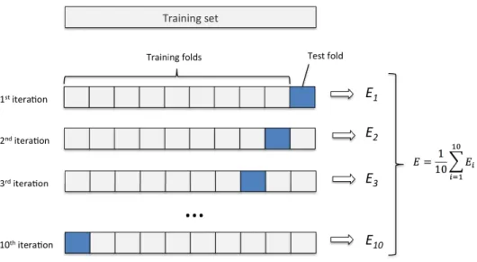
The performance of a model can be validated with a number of techniques. Bootstrapping, jackknifing and cross-validation are the most common resampling methods used in statistics. Cross-validation seems to fit our needs in assessing prediction validity. We asses validity for each response variable separately. Multiple types of cross-validation exist, but we inspect the k-fold cross-validation method.

Cross-validation is used to validate the predictive performance of a model. This is done via error terms. In the k-fold cross-validation, training set is split into k equally sized subsamples. Each subsample is omitted once one

Figure 4.1: Ten-fold cross-validation

at a time as in Figure 4.1. Model processes test fold and compares results to measured values. The difference between predictions and measured values form our error term. This is done as many times as there are subsamples. After all subsamples have been omitted once, the mean of the results is calculated. This mean represents the error of the model.

PLS models validation parameters are R2 _{and Q}2 _{where the first one}

measures ”goodness of fit” and the latter estimates ”goodness of prediction”. We calculate these quantities for each response variable separately in the following equations. R2 _{measures how well the model fits to the data. This is}

calculated using the sum of squares. The Total Sum of Squares (proportional to the variance of the data):

SStot = l

i=1

(yi−y¯)2,

where ¯yis the mean of vectoryandyi is an individual element of that vector. The Sum of Squares of Residuals, also called the residual sum of squares:

SSres= l i=1 (yi−fi)2 = l i=1 ei2,

wherefi is the predicted value from the fitted model at the same point as yi.

The formula of R2 is as follows,

R2 = 1− SSres

SStot

. (4.19)

So ifR2 value is 1 then the model and the measured data would be identical, meaning that the model fits to data perfectly. On the other hand if the value is near to 0 then the model does not fit to data at all.

Q2 is determined by error terms like in Figure 4.1. Parameter Q2 is actually a cross-validatedR2_{, but instead ofSS}

res, the Predictive Error Sum

of Squares (P RESS) is used. Model is built from the data in training folds and P RESS is calculated from the test folds.

PRESS =

l

X

i=1

(yi−fi)2,

wherefi is the predicted value from the fitted model andyi is the real value.

This way Q2 formula is

Q2 = 1− P RESS

SStot

, Q2 ≤1. (4.20)

Value of 1 means that the model predicted test fold values perfectly. Smaller value decreases models predictive credibility. [10] [23]

There are other besideQ2 _{to assess the predictive performance of a model.} The Root Mean Squared Error of Prediction (RM SEP) is a widely used method to measure difference between data and predicted values. RM SEP

is similar to P RESS. RMSEP = v u u u t l P i=1 (yi−fi)2 n (4.21)

The closer the value of RM SEP is to 0, the better.

Measures like Q2 _{and RM SEP should be interpreted carefully. Even if}

Q2 _{were somewhat high in value it does not necessarily mean that the model} predicts perfectly forever. If the new input values are too different from the previous values, one can only hope that the model guesses right. That is, of course, possible if analysed phenomenon has some degree of regularity in it.

For example, some stocks have some regularity in their growth and decline of worth, but some irregularities might cause spikes (anomalies) in value to either direction. These kind of situations are hard for a model to notice if they were not present in the data on which it was built on. In that sense,

R2_{, Q}2 _{and RM SEP are only local quantities.}

4.5.1

Variable importance in partial least squares

projection

The Variable Importance in (PLS) Projection (VIP) is a variable selection method. This way the relevancy of the input variables is measured. The VIP value is namely a weighted sum of squares of the PLS weights, which takes into account the explained variance of each PLS dimension. The VIP of the

jth input variable is VIPj = s nPk a=1R 2_{(y, t} a)(uaj/kuajk)2 Pk a=1R2(y, ta) ,

where uaj is the weight of the jth predictor variable in a component a, k is

the number of PLS components, n is the number of variables and R2(y, ta)

is the fraction of the variance in y explained by the new score ta =Xaua of

a component a. This fraction of the variance is calculated like in equation 4.19. The higher the VIP score the more relevant the variable is. Usually

V IPj >1 is considered good. We use the VIP scores to see if certain input

5

Implementation

In this chapter we experiment with PLS on a dataset to see how the prediction model performs and what other properties of PLS we can use. Simple R-code is provided in Appendix A. This chapter uses ”pls” package from the reference [4]. All images related to analysis are located in Appendix C.

5.1

Technology process

The technology dataset originates from a certain process/processes from Nokia which are kept secret because of legal reasons. The dataset contains 58 input variables and 9 output variables. The dataset has over one hundred thousand observations, but only a fraction of it is used. This is so because it takes a tremendous amount of time to compute such a massive collection of data. We settle on a few thousand observations for the sake of convenience.

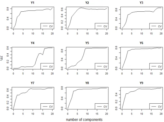
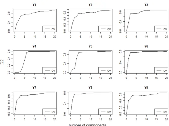
Before we build our model, we must decide how many components we want to use in our model. The number of PLS components can not exceed the number of input variables. Because our case has a large amount of input variables, it is safer to start with many components, so that we see the model improvement clearly. In this case we use 20 components and the results of this are in Figure 7.2. After 6 PLS components the Q2 _{reached good values} in most output variables. All response variables were over 0.5 and some were even higher. It has been proposed that 0.5 is a passable threshold and over 0.75 is a good value [10]. It seems that our model predicts the data well enough. After 15 PLS components Q2 _{does not seem to grow in} most variables. Some variables might improve slightly if more components are used. For example, variable Y1 might get a better Q2 _{value if more} components were used since it seems to increase a bit in Figure 7.2. There is a possibility that slight increase is caused by some statistical irregularity in our data but used training data is somewhat large so it is less likely. Increase happens because the new model component explains some of the variance of Y1. It decreases when unnecessary variation is added that does not explain Y1 but something else. ParameterQ2 _{tends to decrease when a large amount} of components are used resulting a higher variance in a model [10] [7]. This problem is called overfitting. We use 15 components in prediction, because

almost all output variables reach adequate validation values.

To make the predictive performance of the model more clear, Figure 7.3 displays the differences of the model predictions and the actual values. Values on the diagonal line mean that the predicted and the measured values are the same. Values outside of the diagonal line have some deviation from the actual values. Do note that the model predicts some values to be lower than zero. This is obviously not possible in our case since the lower limit of our variables is equal to zero. Regression can make this kind of results which should be corrected or noted in analysis. In Figure 7.3, we see that the model predicts rather well but that there are some outliers. Reasoning as to whether outliers should be retained or deleted from the data is up to the analyst, since they might be results of a normal behaviour of the system. The majority of variables are rather nicely on the line, but Y4 blows up quite a bit compared to others. The model obviously cannot predict it too well. To see things from a different angle we can use residual plot. In Figure 7.4 the difference between actual and predicted values is presented using residuals. This method lets us to inspect the prediction results in clearer manner. Fundamentally, Figures 7.3 and 7.4 hold the same information. Now we can see better if variables are non-linear. It seems that Y3 is a little bit non-linear since it starts to curve down. Y2 also seems to curve but more data is needed to make that conclusion. Variable Y6 seems to have a form slightly similar to a 3rd degree polynomial. Current model being a linear model works quite well despite slight non-linearities but if we try to predict outside our value range then these non-linearities could mean that the results have a large error to them. Y4 variables heteroscedasticity is seen more clearly in Figure 7.4. Heteroscedasticity means that the data population has different variance in sub-populations. This does not affect models variable relations or linear estimates, but the model variance will be biased. There are only mild heteroscedasticities in some of our results so it is not a huge problem but it does lessen the prediction credibility when predicting large values because there is larger error.

The overall importance of the variable in the projection (VIP) is seen in Figure 7.5. Some variables explain more than others. VIP provides a good tool to measure predictors modelling power in the model. Variables X25 and X54 have a very little variable importance in the model due to near zero values. Their proportion might increase if more components were included, meaning that they would actually explain variation in output variables but this is unlikely because both variables are close to 0 at all times in data and