Probabilistic Location Estimate of Passive Mobile Positioning Events

(1)

UNIVERSITY OF TARTU

Institute of Computer Science

Computer Science Curriculum

Joosep Rõõmusaare

Probabilistic Location Estimate of Passive Mobile

Positioning Events

Master's Thesis (30 ECTS)

Supervisor: Toivo Vajakas, MSc

(2)

Passiivsete mobiilipositsiooni sündmuste tõenäosuslik asukoha

hinnang

Kokkuvõte: Uurijad, kes on püüdnud mõista inimeste liikumise mustreid, korjavad andmeid mobiilivõrkudelt. Mobiilid teevad sündmuse kirjeid iga kord, kui nendega helistatakse, saadetakse SMSi või kasutatakse Interneti. Sündmuste kirjed sisaldavad informatsiooni sellest, millisesse võrgu transiiversisse mobiiltelefon oli sel hetkel ühendatud. Võrgu ühe transiiveri leviala saab kasutada, et püüda positsioneerida telefoni geograalist asukohta. Kasutades positsioneerimiseks transiiveri leviala, siis need hinnatavad asukohad pole punktid kaardil, vaid geograalised alad, kus telefon võib olla kui ta on transiiveriga ühendatud.

Mobiilide ühendamine transiiveritega sõltub mitmest muutujast, mis tähendab, et mobiil ei ole alati ühendatud kõige tugevama signaaliga transiiveriga. See teeb mobiili asukoha hindamise keerulisemaks, sest transiiverite levialad võivad üksteisest üleulatuda.

Võrguplaan kirjeldab võrgus olevate transiiverite levialasid ning seda kasutatakse, et de-neerida transiiverite levialasid.

Selles lõputöös hinnatakse mobiilisündmuste positsioneerimise kvaliteeti ruumilise jaotuse ti-hedusfunktsioonidega. Luuakse erinevad võrguplaani variandid ja erinevate võrguplaanide kvali-teeti hinnatakse Bayesi statistikaga ja kasutatakse reaalseid asukoha andmeid. Erinevate võrgu-plaanide kvaliteeti hinnatakse suurima tõepära meetodiga.

Võrreldi RSSI ja Voronoi põhjal tehtud võrguplaane ja nende modicatsioone ja leiti, et Voronoi võrguplaanide puhul paistis asukoha positsioneerimine paremini kui RSSI võrguplaanide puhul.

Lisaks uuriti, kuidas transiiverite levialade üleulatamisel arvestamine Bayesi meetodiga mõjutab asukoha positsioneerimise täpsust. Leiti, et Bayesi levialade üleulatamise meetod tegi halvemate võrguplaanide täpsust paremaks, aga paremate võrguplaanide täpsust halvemaks.

Võtmesõnad: võrguplaan, mobiilivõrk, visualiseerimine, mobiilne positsioneerimine

CERCS: P170 Arvutiteadus, arvutusmeetodid, süsteemid, juhtimine (automaatjuhtimisteoo-ria)

(3)

Probabilistic Location Estimate of Passive Mobile

Position-ing Events

Abstract: Researchers, who are trying to understand human mobility patterns, collect data from cellular telephone networks. Mobiles are creating events every time they are used for calling, SMS, or the Internet. The events contain the information, in which network cell that mobile was at the moment of the event. Cell's coverage can be used for estimating the geographical location of the mobile. The estimated locations are not a point on the map, but the possible area, where the mobile may be when they are connected to that specic cell.

Mobiles connecting to cells are depending on multiple variables, meaning, that a mobile may not always connect to the cell with the strongest signal. That makes estimation of the mobile location more dicult, as the coverage areas may overlap with each other.

Cell plan is a description of cell coverage areas and there are multiple ways for dening cell coverage areas.

This thesis is about estimating mobile events positioning quality with spatial probability density functions. Dierent cell plan variants will be implemented and real ground truth location data is used to nd the modication that maximizes the likelihood estimation.

RSSI-based and Voronoi-based cell plans and their modications were compared. Results showed that Voronoi-based cell plans are better for location positioning than the RSSI-based cell plans.

Furthermore, Bayesian overlapping method was examined to see if applying it would im-prove location positioning accuracy. It was found that applying Bayesian overlapping methods improved the accuracy of the worse cell plans, but made accuracy worse for the better cell plans. Keywords: cell plan, cellular network, visualizing, mobile positioning

(4)

5 Acknowledgment 32 A CDR and GPS x locations with assessments in Estonia and close up in Tartu 36 B Cell Plan Calculator conguration le 37 C Mathematical model of Spatial Probability Density Function 38 C.1 Algorithm for computing the Bayesian PDF of cells and the heat map aggregate statistics using the cells . . . 39

D BEC2016 paper 40

(5)

List of Figures

1 The Illustration of PSTN and hierarchy of its network components [Tiru, 2014]. . 11

2 Cell RSSI decreases with distance increase from the cell site [Agrawal and Zeng, 2010]. 11 3 Best serving data where each cell is in the dierent color [Calabrese, 2011]. . . . 12

4 Voronoi tessellation where the rectancle points are cell sites [Calabrese, 2011]. . . 12

5 Cell plan with cells are colored by the frequency. Dots are the cell sites. . . 12

6 Phone location positioning using cell coordinates[Ahas et al., 2014]. . . 14

7 Users' YouSense event counts per user and per user per month. . . 19

8 Users' CDR event counts per user and per user per month. . . 20

9 CDR GPS counts overview per assessments and per user per assessments. . . 20

10 Voronoi cell plan with gray arrows as cell's direction and brown dots as cell sites. A questionable shape of the cell 3836 is depicted. . . 23

11 RSSI cell with its dBm values example near water. . . 24

12 Relative performance of the various cell plan variants: a) contains cell plans with Bayesian overlapping; b) cell plans without Bayesian overlapping. c) shows eect of the Bayesian overlapping. . . 29

13 Cells SPDF for sequential line of pixels with and without using Bayesian overlap-ping cell model, calculated using Formula 5. . . 30

A.1 Users' GPS x locations with assessments in Estonia. . . 36

A.2 Users' GPS x locations with assessments in Tartu. . . 36

List of Tables

1 YouSense GPS data example. . . 19

2 CDR data example. . . 20

3 Cells basic CSV example. . . 22

4 Cell Plan Calculator input rules le example. . . 25

List of Algorithms

1 CDR and GPS events merging algorithm. . . 21

(6)

List of Abbreviations

A-GPS Assisted Global Positioning System

AML Active Mobile Location

BSC Base Station Controller

BSD Best Serving Data

BTS Base Transceiver Station CDMA Code Division Multiple Access

CDR Call Detail Record

CGI Cell Global Identity

CI Cell Identity

CSV Comma Separated Value

GPS Global Positioning System

GSM Global System for Mobiles

HSPA High Speed Packet Access

HSPA+ Evolved High Speed Packet Access IMEI International Mobile Equipment Identity JSON JavaScript Object Notation

LAC Location Area Code

LBS Location Based Services

LTE Long Term Evolution

MCC Mobile Country Code

ME Mobile Equipment

MLE Maximum Likelihood Estimation

MNC Mobile Network Code

MNO Mobile Network Operators

MPS Mobile Positioning System

MSC Mobile Switching Centers

NMS Network Management System

PDF Probability Density Functions PSTN Public Switched Telephone Network

(7)

RSSI Received Signal Strength Indicator SIM Subscriber Identity Module

SINR Signal-to-Interference-and-Noise Ratio SPDF Spatial Probability Density Functions

TA Timing Advance

UMTS Universal Mobile Telephone System VLR Visitor Location Register

WCDMA Wideband CDMA

WiFi Wireless network

(8)

Denitions of some basic terms.

Mobile network

Base Station Controller - Part of the mobile network. Controls BTSs in a single location area. Handles allocation of radio channels, frequency, power, signal measurements, and handovers within a single location area.

Base Transceiver Station - Mobile equipment access point to the network. Handles speech encoding, encryption, multiplexing and modulation/demodulation of the radio signals. Each BTS has an assigned CGI.

Cell - The geographical area covered by a BTS.

Cell plan - Mapping of each cell in the mobile network so each cell has an approximated geo-graphic area where the ME can connect to that cell. In practice, it is usually dened as a polygon for each cell. In this work we use the same term for the set of continuous SPDF estimates for each cell in the mobile network.

Handover - Changing ongoing call or data session from one BTS to another.

Mobile Equipment - Physical phone or device what is used for connecting to the cellular network. Each ME is uniquely identied by the IMEI number.

Network Management System - Part of the mobile network. Handles administrative and central procedures. Holds data storages warehouses and network handling servers. Mobile Positioning Data - Data collected with mobile positioning about the mobile device

location and movement.

Mobile Switching Center - Part of the mobile network. Controls BSCs. Handles call and messaging routing, updating dierent registries within MSC and the central system, and handovers between dierent location areas.

Statistics

Maximum Likelihood Estimation - MLE is a method of estimating population character-istics from a sample by choosing the values of the parameters that will maximize the probability of getting the particular sample actually obtained from the population. Probability Density Function - The PDF of a continuous random variable is a function that

can be integrated to obtain the probability that the random variable takes a value in a given interval. Formally, the PDF fx(x)of a continuous random variable X is the derivative of thefx(x) = dFx(x)

(9)

1 Introduction

1.1 Motivation

Researchers are trying to understand human mobility patterns. Insight to human mobility could help with dierent issues. In urban planning, understanding how people come and go helps to determine how to build infrastructure, how to reduce trac congestions, or how to reduce pollution. Knowing people home and work locations, helps to plan commuting routes between work and home. In medicine, it could help to understand how some disease spreads. Human movement data is needed to analyze this kind of problems. Collecting that data traditionally is costly. Doing movement surveys and direct observations need time, money and usually, result in small sample sizes [Becker et al., 2013].

A simpler way to collect data is to use the Mobile Network Operators (MNO) collected positioning data. Most people in the world use mobile phones and MNO collects events made when mobiles are used for SMS, calling or the Internet. These events metadata includes the cell tower where the mobile device was connected at the time of the event. This data is collected for other purposes but the location info can be used for positioning the mobile devices [Tiru, 2014]. The cell tower is at one point on the map, but that does not mean that the mobile device is there. Location positioning accuracy could be 100m to 1km in urban areas and in rural areas up to 30 km [Saluveer et al., 2012]. To describe the possible location area for the mobile device, that is connected to some cell, cell plans are used to visualizing cell eective area coverage. MNOs usually have details following: each cell tower location on the map; which direction each cell on the tower is facing; other cell describing attributes [Tiru, 2014]. What they do not always have is eective area coverage information. For that dierent algorithms are used for generating that area.

1.2 Structure of the thesis

Chapter 1 has the introduction. It gives an overview of the topic, describing cellular network and mobile positioning data. After that, there is described what has been previously done in this topic research and what this thesis will add to that. Chapter 2 describes the data and dierent methods what are used in this thesis. Chapter 3 shows the results of the thesis and Chapter 4 contains the conclusions and the discussion about the results.

1.3 Background

1.3.1 Description of the eld

Mobile technologies. To call another person, you need a mobile phone and the network connection. So the rst thing you need is Mobile Equipment (ME), that is your physical phone or device what is used for connecting to the cellular network. Each ME is uniquely identied in the network by the International Mobile Equipment Identity (IMEI) number. In Europe, everyday phone users do not encounter this problem, but ME must be able to operate on a cellular network. There are two basic technologies in mobile phones: Code Division Multiple Access (CDMA) and Global System for Mobiles (GSM) [COAI, 2016].

Segan [Segan, 2015] describes what technology you need when you want to buy a new phone in the United States. In Europe, GSM radio system is used. Problem is that with GSM carriers verify users with Subscriber Identity Module (SIM) card and CDMA carriers use network-based whitelists. Phones with only GSM support can not operate in CDMA networks and vice-versa.

(10)

Besides that when you change the phone you just have to take out the SIM in GSM phone and put it into another phone. In CDMA you need carrier's permission to change the phone.

The main dierence is in the core radio signaling technology. CDMA uses spread spectrum signal encoding, which transmits data of each subscriber over the entire frequency spectrum of the antenna all the time, while GSM assigns a time slot for each subscriber's data where no other subscriber can have access [Tiru, 2014]. In CDMA code division each subscriber unique key is assigned which is used to decode combined signal into its individual calls. In GSM time division subscriber pieces the call back together from assigned time slots.

Code division method need more processing power, but is more powerful and exible technol-ogy and when GSM was upgraded to 3G, it started to use CDMA technoltechnol-ogy, but it was called Wideband CDMA (WCDMA) or Universal Mobile Telephone System (UMTS). WCDMA uses wider channels than CDMA (like the name suggests) but has more data capacity. To increase data transfer speeds, GSM 3G was upgraded to High Speed Packet Access (HSPA), which is known as 3.5G. Later HSPA was upgraded to Evolved High Speed Packet Access (HSPA+)(3.75G).

Both systems will be soon upgraded to a common global standard named Long Term Evo-lution (LTE). LTE is globally accepted 4G wireless standard. Report [OpenSignal, 2016] shows that currently there are 148 countries with LTE networks and 10 countries are scheduled to go online with LTE networks. First LTE network was deployed in Estonia 2010 by Telia (then named EMT), and all three main MNOs had LTE support from the beginning of 2013.

Besides technological platforms CDMA, GSM or LTE, there are also dierent standards and protocols that must be supported by the mobile devices. This includes network generations 2G, 3G, 4G and frequency bands that they work in. 2G was rst digital network and had added a link to the Internet. 3G increased the communication speed and added various value-added services like video calling, live streaming, mobile internet access, etc. 4G (also known as LTE) enabled ultra-broadband Internet access, gaming services, and high denition television [Tondare et al., 2014].

In Estonia, 2Gs is supported on bands GSM 900, GSM 1800, 3G on UMTS 900, UMTS 2100, 4G on LTE 800, LTE 1800, LTE 2600 [GSMArena, 2016]. Numbers behind the technologies are showing in what frequency band they are working (i.e. 900 means that it works in a frequency band that is near 900MHz).

Public switched telephone network Mobile equipment connects to the network by the Base Transceiver Station (BTS). It is the antenna that is on top of the radio tower. It carries out radio communications between the network and the mobile equipment. It handles speech encoding, encryption, multiplexing and modulation/demodulation of the radio signals [Tiru, 2014]. BTS has an assigned CGI value. CGI is made of four identication values: Mobile Country Code (MCC), Mobile Network Code (MNC), Location Area Code (LAC) and Cell Identity (CI). MCC shows in what country cell is location, MNC to which network operator it belongs to and LAC shows in which location area it belongs. CI shows cell id, depending on MNOs it may be unique over all network or unique in LAC [shareTechnote, 2016].

There are two types of BTSs: directional and omnidirectional. BTSs have usually the directed antennas and one BTS covers 120-180 degree sector of an area and a tower with 3 BTSs will cover all 360 degrees. Depending on use cases one tower could also hold only one or two BTS with dierent sector degrees and for redundancy one tower could also be serviced by several overlapping BTSs. Omnidirectional antennae transmit in all directions and are usually alone on their tower [Kwan et al., 2012].

Base Station Controller (BSC) controls a number of BTSs in a proximate geographical area, that is BTS in a single location area. BSC handles allocation of radio channels, frequency, power and signal measurements. If ME changes BTS in a single location area, then BSC is responsible

(11)

Figure 1: The Illustration of PSTN and hierarchy of its network components [Tiru, 2014]. for handover procedures. Handover is changing ongoing call or data session from one BTS to another.

BSCs are controlled by Mobile Switching Centers (MSC). MSCs are one or many, depending on the size of the MNO. MSC handles the call and messaging routing, updating dierent reg-istries within MSC and the central system and handover between dierent location areas and MSCs. MSC also contains Visitor Location Register (VLR). VLR is the registry for holding the information about the location area and the BTS to which ME are connected.

MSC reports to the Network Management System (NMS). All the administrative and central procedures are done in NMS. Data storage warehouses and network handling servers are also there. This network with connections to the other MNOs is called Public Switched Telephone Network (PSTN) and is illustrated in Figure 1.

MNOs could share some of the network equipment and network modules between themselves (e.g. it is not uncommon to share the antenna between MNOs). There are even virtual MNOs that do not own any network infrastructure but rent it from other MNOs [Tiru, 2014].

Figure 2: Cell RSSI decreases with

distance increase from the cell site [Agrawal and Zeng, 2010].

Cell plan. Each BTS has a Cell Identity (CI), like was mentioned in the last subsec-tion. Cell is a geographical coverage area, where ME could connect to that cell BTS. Ra-dio tower where the BTS is connected is called the cell site. The cellular network is made of BTSs and their cells, hence the name. Each cell can cover a limited number of ME within the cell coverage area. Capacity is limited by available bandwidth and operational require-ments. To give the best user experience, MNO has to add or remove BTSs and size cells after the need to handle expected trac demands [COAI, 2016].

BTS with omnidirectional antennae tend to have cell with a hexagonal pattern, di-rectional antenna is ofter diamond-shaped [Kwan et al., 2012]. But in real world shapes

(12)

con-nects to a BTS over radio signal, so probability for ME to connect to a specic BTS is depending on Received Signal Strength Indicator (RSSI). Signal strength is measured in dBm, further the ME from BTS is, the lower the dBm value. RSSI change with cell's distortions and overlapping is illustrated in Figure 2 [Agrawal and Zeng, 2010].

Figure 3: Best serving data where each cell is in the dierent color [Calabrese, 2011].

Figure 4: Voronoi tessellation where the rectan-cle points are cell sites [Calabrese, 2011].

Figure 5: Cell plan with cells are colored by the frequency. Dots are the cell sites.

When ME is close to the edge of a cell, where RSSI is low, then handover occurs and ME is serviced by another BTS. When ME is near the edges of multiple cells, then ping-pong eect may occur, meaning ME will be switched from one BTS to another multiple times in a row. For ME user everything works ne, but by BTS positioning, it will show that ME location starts jumping fast from one cell to another [Vajakas et al., 2015].

Cell size depends on its frequency and type. Higher frequency cell's strength will de-crease faster than with lower frequency. Cells are categorized by their size from largest to smallest: macro, micro, pico, femto.

Macro cells main purpose are to cover large areas. Radius may be up to several kilometers. Generally most rural and suburban areas are covered by macro cells.

Micro cells are mostly used in urban areas with a radius of hundreds of meters. They are deployed to places with higher trac densities, e.g. large shopping malls.

Pico cells are small cells with radius up to tens of meters. Used in places with very high trac volume, e.g. train stations or of-ce buildings. BTS of pico of-cells tend to be omnidirectional.

Femto cells are smallest cells that are used in residential indoors where the mobile opera-tor network may not be provided by the oper-ator. Instead, it may be connected to the dig-ital subscriber line (i.e. digdig-ital data is trans-mitted over telephone lines) .

These categories are complemented with two additional types: umbrella and metro cells. Umbrella cells are the combination of larger cells with several smaller cells, where a larger cell is used for providing coverage and mobility between smaller cells. Metro cells are very similar to micro cells, but metro cells in-tegrate all elements required for the BTS oper-ation in one compact device [Penttinen, 2015]. Cell plan is the mapping of each cell in the

(13)

to that cell [Vajakas et al., 2015].

CDR gives a cell ID, usually in a form of CGI) where the ME was connected on when some event happened. That ID gives the cell site geographical location. When BTS is omnidirectional, then site's location could be good enough for ME location, because it is in the center of its coverage area. When BTS has a directional antennae, then BTS is at the corner of the coverage area and mostly ME is somewhere else when it is connected to that BTS. More precise positioning would be using the center of the coverage area geometry. There are two methods to get the cell geometry. One is to measure or calculate RSSI measures for any geographical location. MNOs have special programs for generating best serving data (BSD). Best serving data is cell map that takes into account cell sector and propagation models and is made on simulated coverage. Each location in a grid is associated with the BST which covers that location best as shown in Figure 3 [Calabrese et al., 2014]. This method assumes that when ME is in some location where some BTS has the best serving (RSSI value is better than other cells), then ME would connect to that cell.

Another way to create the cell geometry is a more simple way without the need for radio measurements. Free-space propagation is assumed with that all BTSs have the same equivalent radiated power. With these assumptions, Voronoi tessellation technique could be used on the cell site locations. Voronoi tessellation partitions the space into cells based on the distance between each point and the closest BST. Set of points that are closer to the one BST than others is included to that cell [Csáji et al., 2013]. Resulting graph is shown in Figure 4.

Cell plans in real world are not so clear as in Figure 3 and Figure 4. As mentioned before, cells can have dierent frequencies and sizes. They can also overlap to produce better coverage. Cells with dierent frequencies do not form cellular-like network, because it is not unusual that on the same tower two directional BTSs with dierent frequencies or technologies are directed in the same direction. When taking into account all the frequencies and technologies that are used in building the mobile network, picture would be more as seen in Figure 5, where each technology with its working frequency (e.g. GSM900, UMTS2100) are shown using dierent color for each dierent technology.

Mobile Positioning Data. Collecting people location information by surveys and observation is too resource-consuming work, a cheaper method for data with bigger sample size would be mobile data. That is considered most promising data source for measuring the mobility of people [Tiru, 2014]. Most people in the world has a mobile phone. There are 5 billion subscribers to mobile networks. Subscriptions devices itself has reached 7.4 billion. Which means that there are more devices connected to the mobile network than there are people in the world. And that num-ber is growing around 3 percent per year. That numnum-ber is so large due to inactive subscriptions, multiple device ownership and subscriptions for a dierent type of calls [Ericsson, 2016].

Mobile devices can be used for collecting their location data with mobile positioning. The mobile positioning means that it is possible to locate devices in time and space with certain accuracy using technology (e.g. mobile network infrastructure or Global Positioning System (GPS)) to get the location of the mobile device. That data about the location and movement of mobile devices is called mobile positioning data.

There are three methods for collecting data. 1. GPS and Assisted GPS (A-GPS)

2. Wireless network (WiFi) location databases 3. Network antenna-based location database

(14)

Assisted GPS is used to speed up rst GPS location calculation. Usually using WiFi and net-work antenna-based location databases to pinpoint device location before getting a more precise reading with GPS [Waadt et al., 2010]. WiFi and network antenna-based location databases use information about where the given network antenna or WiFi transmitter geographically is located to predict mobile device location. WiFi and network antenna-based locations are used when there is not possible to use GPS location. As for GPS to work, there must be line-of-sight to at least three GPS satellite. So GPS do not work indoors and in the urban canyons created by buildings on either side of a street [Mountain and Raper, 2001].

Network antenna-based location database system with common name Mobile Positioning System (MPS) is used by MNOs to pinpoint the location of the mobile phones using network infrastructure. There are dierent methods to locate a mobile device [Tiru, 2014].

• Cell Global Identity (CGI)

• Trilateration of antenna to device and back • Angle of received signal

• Timing Advance (TA - radio signal arrival time from antenna to device and back)

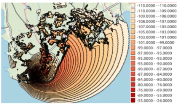
A mobile device knows to which cell it is connected and what is that cell's CGI. From MNO side they can see to which cell the mobile device is connected and what is the cell's identication. From that MNO can look what is that cell's geographical location and know that the mobile device must be somewhere near the cell's location as seen in Figure 6. Trilateration is three sites to pinpoint the location of a mobile device. The angle of received signal uses an array of smart antennas that help to determine the angle of the incoming radio signal. Then it is possible to triangulate known signal angles from at least two base stations. Timing Advance takes into account time needed for the signal to reach mobile device and back to cell station [Ratti et al., 2006].

Figure 6: Phone location positioning using cell coordinates[Ahas et al., 2014].

Most commonly CGI+TA+angle of re-ceived signal is used, where cell's location is rst found after cell's identier and after that TA is used for calculating how far the mobile device is from the cell tower and direction of the device is determined after the angle on re-ceived signal [Tiru, 2014].

Mobile positioning data can be collected with two dierent methods: active positioning and passive positioning.

Active positioning. Active positioning needs active request and usually requires au-thorization from device owner. When the po-sitioning request is made then device owner has to give the consent for the request. Most people have seen location request pop-ups on applications and map-related websites or user had to approve location request when in-stalling the application . There are also re-quests made without user consent. User authorization is not needed if location request is done in the case of emergency. That usually means using MPS, but from July 2016 Estonia and

(15)

the United Kingdom have implemented the Active Mobile Location (AML) system. AML is emergency call-based location solution in Android phones. When smartphone recognizes that an emergency call is made, then phone activates its location services and sends that info to the emergency services automatically before turning the location services o again [EENA, 2016].

Most usual active positioning is installed applications ability to use the location of the mo-bile device and positioning work real-time or near-real time. Location Active positioning has beneciaries from dierent user groups [Ratti et al., 2006].

Active positioning applications can be divided by their target group of users.

• Services for individual users

Navigation aids

Geographically distributed yellow pages Educational services

• Services for group of users

Distributed chats and friend tracking Location-based gaming

Trac services Digital tapestries Coordinated actions

• Services for third parties

Public safety and security Family security

Emergency relief

Business safety and eciency

Commercial and information services Location sensitive billing

Urban Systems mapping

There are dierent applications that are used where location positioning is the main intention, but there are other applications where location data is still collected for value-added services or statistics. Social media applications (e.g. Twitter and Facebook) do not always need location data, but the data is still collected [Tiru, 2014].

There are advantages and disadvantages to active positioning compared to passive positioning. Just like with in person, on-line or telephone surveys, active participation could be requested and sampling techniques could be used. Data collection is easy because participants only need to install positioning application to their phone or approve the periodical network-based location requests. The disadvantage is the need to recruit the respondents, resulting small sample size [Tiru, 2014].

(16)

Passive positioning. The dierence in a passive and active positioning is, that passive positioning does not need to send a request to a mobile device, to position it. Instead of actively making position request, data is already collected to some database by the MNOs or applica-tions. This data usually is not collected with the purpose to collect the location. Applications and MNOs are logging mobile devices activities and these logs can have data that could be linked to a location [Tiru, 2014]. This data is used mostly internally for business and marketing purposes (e.g. billing clients, providing statistics, marketing). Location data is used seldom [Ahas et al., 2011].

Passive mobile positioning data is mostly referred to the data from MNOs. MNOs are col-lecting a lot of business purposed data, among them are Call Detail Record (CDR). One CDR contains a lot of technical information about the recorded activity, but the important elds are subscriber identication, time of the event and identication of the antenna, where the mobile device was connected at the time of the activity. CDRs include in and out calls, SMS and MMS messages activities. If mobile devices use also Internet trac, then these activities are also in-cluded in CDR. MNOs can choose what data they want to store and because of that data about mobile devices locations and how precise could location detection be may dier. The size of the data may also vary, meaning that MNOs may store only 2-3 CDRs or even 200-300 CDRs per mobile device per day.

People carry their mobile devices always with them, so CDR data gives an overview of human movements based where they are using their phones. MNOs have also extra info about their subscribers, there may be also access to additional data about the socio-demographic prole (e.g. gender, age) for each mobile device owner.

The main advantages compared to active positioning is the cost-eectiveness of collecting a large sample of data for all the phone users. With passive data collecting, there is no burden on the respondents because data is collected automatically [Ahas et al., 2011]. Access to that data is more dicult. That is because of privacy. People do not like that other people get access to that sensitive data like their location history. At the same time, MNOs do not like to share their data on business related reasons. If MNO would give their CDR data for research, then it would still not contain the full sample of the whole country. One country can have more than one MNO providing their services (e.g. Estonia have three main MNO companies: Telia, Elisa, Tele2). If selecting only one company then sample contains only their clients and mobile devices that uses their cellular network [Tiru, 2014]. Another problem is the CDR data itself. Even if the data size is very large, data accuracy itself is not as good as with GPS collected data. In practice, most CDRs do not have enough information to use more precise positioning methods like using TA or angle of signal arrival because they need more than one base station, but only the base station that is carrying mobile communications are recorded in CDRs [Zang et al., 2010]. Data privacy. A big problem with Location Based Services (LBS) is that people do not like that their movements can be tracked. To encounter that problem there are two solutions. One is asking each person's permission to track them for research purposes. But this means small sample size because you have to interact with each one. A second way is to anonymize the data. That means there is not possible to connect the data with the person whose data it is. Ratti et al. [Ratti et al., 2006] shows the European Union directives, that ensures people privacy rights. There are very precise cases when service providers could work with people's privacy data and when they can give it to third parties. With the European Union directives they can only do that when they have the consent of the service user and the user is informed of the purpose and duration of the process. Another way is to analyze and to give that data to the third party to analyze it, is to anonymize it. Most researchers working with MNOs mobile positioning data are using anonymized and aggregated data.

(17)

Datasets are anonymized to bypass the problem of privacy, so researchers can not track data back to the user to whom that data belongs. Researches like [Ahas et al., 2007, Ratti et al., 2006, Ahas et al., 2011] have to use it to work with the data without the breach of privacy. Ahas et al. [Ahas et al., 2011] and Tiru [Tiru, 2014] bring out the problem, that anonymizing could lose the dierent aspects of the data, that could be useful to research. Wicker [Wicker, 2012] brings out that anonymizing must be done correctly because with location traces could be de-anonymized through correlation with publicly available databases.

Besides the people's data privacy, another big problem is MNOs business secrets. They do not want to share their cell tower locations and information to others. In this thesis users and cell towers identications and are changed because of privacy issues. Cell towers real geographical locations are also hidden.

1.3.2 Related work

Passive mobile positioning with CDRs has been used for some time.

Articles [Mountain and Raper, 2001] and [Ahas et al., 2007] used it to research seasonality of foreign tourists space consumption in Estonia. Article [Ratti et al., 2006] used it to analyze urban activities in Milan, Italy. Article [Saluveer and Ahas, 2014] describes how passive mobile positioning can be used to nd peoples home and work location. But it also mentions that there are accuracy problems and discusses what kind of extra information should be added to MNOs CDR data, to get the more precise location prediction (i.e.. take into account that ME location probability is higher in the places where there are roads, point of interests or buildings.)

Article [Vajakas et al., 2015] used passive mobile positioning with CDR data to reconstruct people movement trajectories.

Using Voronoi with clustering close BTSs together was used as a cell plan in [Csáji et al., 2013]. They used Voronoi-based cell plan with only omnidirectional cells. They took into account that ME may be in the other cell area not in the one, it is connected to. They proposed to use BSD information instead of simple Voronoi. They also used Maximum Likelihood Estimation (MLE) for estimating the position of frequent locations.

Article [Zang et al., 2010] described the methodology applying Bayesian methods for dening the Spatial Probability Density Functions (SPDF) for mobile positioning. Estimation was based on Signal-to-Interference-and-Noise Ratio (SINR) calculations. Bayesian probability estimate was provided for the situations where CGI was the only information to know and no other cells had good enough SINR. The method was tested on the subset of emergency call data, that was limited to situations where only one cell was within the reach of the BTS. They found that the dierence between the location measured by the GPS and the MLE provided by that method was improved by 20%, compared to the baseline method. No direct Probability Density Functions (PDF) tests were performed and they did not consider that the probability to connect to a specic cell will be reduced where other cells are reachable.

Unpublished paper [Vajakas and Vajakas, 2014] created SPDF estimations with Bayesian rule method. Formulas were created that took into account that probability to connect to a concrete cell will be reduced in locations where other cells are reachable, but the paper was lacking in real world tests.

1.4 Contributions of this work

This thesis concentrates on algorithms on how to position mobile devices from CDR information. Dierent cell plans creation methods are described and tested with mobile device GPS location and connected cell CGI data.

(18)

Passive mobile positioning SPDF estimations are used for comparing quality of the cell plans. This thesis continues the work [Vajakas and Vajakas, 2014] which started the research on SPDF estimations with Bayesian rule. Important part of the article is added to the appendix C. SPDF estimations methods with and without Bayesian rule are used to verify if the cell plan overlapping is important.

The theoretical foundation of SPDF and application of Bayesian rule were devised by Toivo Vajakas (original ideas) and Jaan Vajakas (ensured mathematical correctness).

The author applied and adapted the theoretical base to concrete technological stack in Reach-U: devised conversion algorithms for concrete cell plan inputs, implemented the algorithms for cell plan data processing and evaluation (except the code described in appendix C), analyzed the results.

Paper [Vajakas and Rõõmusaare, 2016]1 _{will be published based on the theory of SPDF}

es-timations with Bayesian rule and the results of this thesis. Paper that was sent to the review is included in the Appendix D.

1_{Jaan Vajakas was not included as an author, because as a Google Inc employee, he did not have time to get} permission from Google Inc.

(19)

2 Methods

2.1 Description of the data

2.1.1 User data

There were ve test users with the identications 1,2,3,5 and 6. Data collection time period was almost 8 months: 01.04.2015 - 18.11.2015. User 4 only collected the YouSense data for the rst month, and because of that this users data was discarded.

YouSense data. GPS and connected cell information were collected from our test users with android application YouSense, an active positioning application created by the company OÜ Positium LBS.

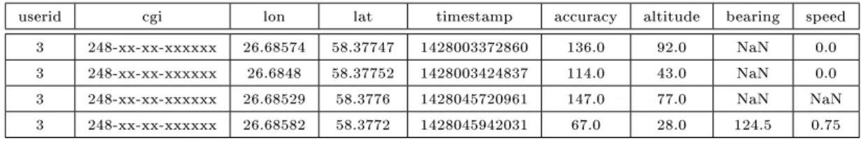
Example collected data is seen in Table 1. The timestamp is in Unix epoch milliseconds. the application collected GPS locations every 1 second if ME was moving faster than 3 m/s and every 16 seconds if it was moving slower than that. The application turns GPS tracking o when ME moves less than 20 meters in 4 minutes or GPS x could not be obtained for 60 seconds. When ME starts moving again, GPS tracking will be turn on. There may be caps in the collecting when the ME do not have its GPS turned on.

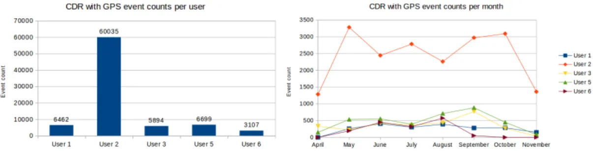
Figure 7 shows how many GPS events each user collected in the whole period and how many events each month.

userid cgi lon lat timestamp accuracy altitude bearing speed 3 248-xx-xx-xxxxxx 26.68574 58.37747 1428003372860 136.0 92.0 NaN 0.0 3 248-xx-xx-xxxxxx 26.6848 58.37752 1428003424837 114.0 43.0 NaN 0.0 3 248-xx-xx-xxxxxx 26.68529 58.3776 1428045720961 147.0 77.0 NaN NaN 3 248-xx-xx-xxxxxx 26.68582 58.3772 1428045942031 67.0 28.0 124.5 0.75

Table 1: YouSense GPS data example.

Figure 7: Users' YouSense event counts per user and per user per month.

CDR data. With our test users permission, we also collected their CDR data from MNO for the same period as GPS data. CGI values are used for positioning from CDR data because MNOs do not always have better CDR data for passive mobile positioning than just a CGI value. The example of the data is seen in Table 2. the timestamp is in Unix epoch seconds. CDR contains events with dierent types, this is given in the event column. They could be call, SMS, location update, etc. This thesis does not take event type into account for positioning.

(20)

Figure 8: Users' CDR event counts per user and per user per month.

Figure 9: CDR GPS counts overview per assessments and per user per assessments. Figure 8 shows how many CDR events each user made in the whole period and how many events each month.

userid timestamp MCC MNC LAC CI Event type

3 1427856959 248 xx xx xxxxxx 85

3 1427900159 248 xx xx xxxxxx 85

3 1427980327 248 xx xx xxxxxx 18

3 1427980332 248 xx xx xxxxxx 85

Table 2: CDR data example.

Combining CDR events with GPS data. A program was created to merge CDR and GPS events. It reads in CDR events and uses GPS data to nd the ME's real geographical location. For each CDR event, GPS event x will be created based on the GPS events before and after the CDR event time. GPS location selection process is described with Algorithm 1. Each selected GPS event x has an assessment for how precise that GPS could be. Overview of the result is given in Figure 9.

GPS xes points locations are showed in the Appendix A. Figure A.1 shows location points over Estonia and Figure A.2 shows close up in Tartu, where the majority of events were made. There are big lines from yellow dots with assessment Too far in time that show how unrealistic these measurements are. CDR events with GPS xes with assessment Too far in time and Too far in location were discarded. That means from all the events there are 37370 useful CDR events with GPS xes.

(21)

Algorithm 1 CDR and GPS events merging algorithm.

For each user:

• Remove CDR events that are outside of the GPS events time frame, because extrapolation is not supported. • For each remaining CDR event :

Use binary search over time-sorted GPS events to nd the GPS event with the smallest time that is larger or equal to the CDR event time.

Found GPS event will be known as the next x.

The GPS x before the next x is known as the previous x.

∗ If the next x is the rst recorded GPS event, then it will be used as the previous x and the next GPS event after that will be the next x.

Calculate interpolated GPS x.

∗ The interpolated GPS x values are a weighted average of the previous and the next x with the time of the CDR event.

· Each GPS x weight is time dierence from the GPS x time to the CDR event time.

Select assessment for the interpolated GPS x.

∗ If the previous and the next x are farther than 15 minutes from the CDR event time, then assessment is Too far in time.

∗ If the previous and the next x are both closer than 10 seconds from the CDR event, then: · if both xes are farther from each other than 100m then Too far in location is chosen. · if both xes are closer than 100m, then interpolated x is chosen.

∗ if the previous and the next x are closer than 15 minutes from the CDR event, then: · if the previous x is closer than the next x, then previous x is chosen. · if the next x is closer than the previous x, then next x is chosen.

Select GPS x based on the assessment.

∗ With assessments interpolated x, Too far in location and Too far in time, interpolated GPS x is chosen.

∗ With assessments previous x, previous GPS x is chosen. ∗ With assessments next x, next GPS x is chosen.

2.2 Cell plan creation techniques

Cell plan can be generated using multiple dierent approaches.

What method to use depends on the cell plan's purpose. If it would be used for analyzing network coverages, then cell plan that includes cell's fringe areas could be better. If it would be used for showing the area where the ME more likely was when it was connected to that cell, then smaller cell size would give a better location estimation accuracy. This thesis uses cell plans for positioning ME locations.

Cell plan generation methods in this thesis and the implementation of them are created for application Demograft. Demograft is a tool for MNOs that uses passive location data of their customer base to help them analyze their network. It also helps them selecting subscribers for advertising campaigns. Demograft was developed by Reach-U [Reach-U, 2016] and STACC [STACC, 2016].

When the nal intention of a cell plan is known, then generation depends on the available cell data. Simplest data would be cells identications and their geographical locations. This will give the most inaccurate cell plan because as there is not any information about the direction of the cells. So all the cells could be generated as omnidirectional and the cells on the same

(22)

site would have the exact same cell geometry. If data includes direction of the antenna, then directional cells could be generated and cells on the same site could each have the cell geometry in the correct direction. If frequency or technology is included, then each dierent frequency and technology could have cell plans on separate layers. More cell attributes help to generate more precise cell shapes. This information is usually given in a Comma Separated Value (CSV) or an Extensible Markup Language (XML) le.

When MNOs have the BSD les or RSSI data and they are prepared to share them, then this data could be used for generating more real-world-like cell plans. To generate cell plans from dierent inputs Cell Plan Calculator was created for Demograft application. This chapter describes the methods used by Cell Plan Calculator to create cell plans from dierent input data. 2.2.1 CSV le input

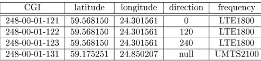
The basic information for each cell is usually given by the MNOs with simple CSV or XML le. Most CSV or XML les contain cells geographical points(cell site coordinates) with descriptive metadata. As cell plans are made of geographical coverage areas, then we have to generate areas from given cell location point and its metadata. Minimum requirement information for each cell are location coordinates and a cell's CGI, but to get realistic cell shapes, then direction and frequency is also needed. Basic cell table is shown in Table 3.

Longitude and latitude coordinates for the cell are needed for the site location, without it, there is not possible to know where the cell should be located on the map.

Direction shows in where the cell is pointed. Missing direction value should show that given cell is omnidirectional cell and does not have direction (in the Table 3 shown as null) . If the direction is missing for whole data, then we can only assume that every cell in the given data is an omnidirectional cell.

The frequency for each cell is important because cells in dierent frequency band should be separated from each other. If frequency info is missing, then we have to assume that every cell is in the same frequency. Sometimes instead of frequency column, each frequency is given in a separate le.

CGI latitude longitude direction frequency

248-00-01-121 59.568150 24.301561 0 LTE1800

248-00-01-122 59.568150 24.301561 120 LTE1800

248-00-01-123 59.568150 24.301561 240 LTE1800

248-00-01-131 59.175251 24.850207 null UMTS2100 Table 3: Cells basic CSV example.

These requirements are minimal but may not be sucient for a more precise cell plan. There may be more information given to each cell. If a cell radius is also given, it can be used for not letting the cell spread top far. With a cell type, we can tell how big cell area should be and even could help for deciding if a cell is omnidirectional or not. Normally, the direction eld should be enough for knowing if a cell is directional or not, but the practice has shown that MNOs cell data is not always perfect and having more information about cell's attributes, helps to make better decisions for creating cell area for each cell.

Using the basic information, there are three ways to generate cell plan. Each method will create cell plans with dierent geometry shape.

(23)

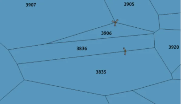
Figure 10: Voronoi cell plan with gray arrows as cell's direction and brown dots as cell sites. A questionable shape of the cell 3836 is depicted. Voronoi cell plan. The Voronoi method is

used for generating cell plan that does not have overlaps between cells in the same fre-quency. This creates good areas for mobile po-sitioning but does not take into account that in reality cells will overlap. This can be xed by enlarging each cell after generating Voronoi cells.

This method is a fast way to divide whole coverage between each cell, but may create some irregular shapes, Figure 10 shows big cell number 3836 that is narrow in the west-east direction, but the cell direction is almost to the north.

Voronoi cell plan creation algorithm is de-scribed in Algorithm 2.

Algorithm 2 Voronoi cell creation algorithm.

For each BTS technology and frequency do following: • Separate omnidirectional BTS from directional BTS.

• Create omnidirectional BTS cell hexagon geometry based on BTS cell's radius. • Cluster directional BTS that are close to each other together.

This is used because MNO does not always site information for BTS. • Cluster center point will be cell site for each BTS in that cluster.

• Each BTS location will be moved a little in the direction of that BTS cell direction.

This will force Voronoi diagram builder to build cells for each BTS in the correct direction (one cell site will have correct sectors).

• Add moved BTS locations to Voronoi diagram builder. • Build Voronoi diagram

• For each BTS:

Find geometry in Voronoi diagram that has BTS moved location inside it. ∗ That geometry will be that BTS cell.

∗ Cut cell geometry with that hexagon with BTS maximum radius.

Set BTS site location back to its original location.

2.2.2 CSV and best serving data les input

MNOs provide sometimes so-called best serving data in raster format. Each frequency cells are in separate layers. BSD example was shown in Figure 3. For working with each cell geometry, these les must be rst converted from raster to vector format. This is done with ogr2ogr tool [ogr2ogr, 2016]. As with Voronoi method, there are no overlaps between cells in the same frequency. Again cell enlargement modication could be added for each cell after creating the

(24)

cell plan.

CSV les are still used for extra cell plan info, but the geographical areas are taken from the BSD raster les.

2.2.3 CSV and RSSI les input

Figure 11: RSSI cell with its dBm values exam-ple near water.

As with BSD data, CSV les are used for all the extra cell attributes, but geographical data is taken from the RSSI data. RSSI data is the biggest in data volume. Each cell in the net-work has very precise geometries where each geometry has RSSI what value that cell should have in that geographical location. Figure 11 shows one cell RSSI values on the map. MNO holds this data in databases and it needs a little bit more preprocessing before Cell Plan Calculator could do anything with it. First signal strengths period is selected, usually, pe-riod -80...-83dBm is selected. Per each cell all the geometries that have the RSSI value in se-lected period would be downloaded from the

database and the convex hull algorithm will be applied to these geometries. The resulting geom-etry is polygon where all the selected geometries are inside of it. Shapele is created from these polygons and that is used like in the BSD method.

Each cell area was selected according to its RSSI value. Unlike BSD, the cells derived from RSSI data can overlap in the frequency band. This method could leave some uncovered holes in the whole cell plan coverage - there may be areas where each cell RSSI value is lower than selected period, this could be improved with selecting RSSI period with lower decibels.

2.2.4 Cell Plan Calculator

Cell plan Calculator takes in a conguration le in JavaScript Object Notation (JSON) format. Everything necessary for its work is described there, but extra ags can be added to change calculator behavior. There are ags for changing the output le location for easier automation scripts. MNOs are changing their network day-to-day to adjust to subscribers needs and because of that cell plans need to be up to date with real world situation.

Cell plan generator was built to work in ve steps. Generation could skip some steps if they are not needed for some specic MNO.

Parsing CSV les. First step is parsing CSV(or XML) input les. This step will read in one or more CSV les. Each le can be described separately to the calculator in the conguration le. As MNOs congurations and cell data les may vary then conguration le is made to be very exible. A conguration le example is in Appendix B. The conguration le is used for reading CSV les in and then converting them to a specic form that all the next step can use. Parsing rules. Rules are used for conguring two things: cell's radius and its boolean value with true if a cell is omnidirectional and false if it is directional. It is used when input le does not have a radius or omnidirectional attribute info. Rules are described in a separate le, which location is given in conguration le. An example of the rules le is given in Table 4.

(25)

Table 4: Cell Plan Calculator input rules le example.

Rules le contains three columns, sepa-rated by a pipe character. The rst column has a resulting radius. Radius is used for lim-iting cell areas from reaching too far from the cell site. It is used when generating omnidi-rectional cells: a radius is used for polygons radius and if Voronoi cell is very large, then it is also trimmed with radius. Radius depends on dierent things, for example, cells with dif-ferent frequencies have dierent reaches. The

second column has resulting omni cell boolean value. If the boolean value is true, then Cell Plan Calculator will generate that cell as omnidirectional. Otherwise, it will be counted as a directional cell. The last column holds the expression for given rule.In expressions, conditionals are described for the cells. if they match with cell's attribute, then selected radius and isOmni parameter values will be chosen to that cell.

The tool will start testing expressions from the rst one and if expression fails, then will be moving to the next one. If successful validation has been found, then that radius and omni cell values will be used. e.g if the rst expression is successful, then it would not try the next ones. The last one in the list should be the default value if other expressions have failed.

Expressions are written in MVEL [MVEL, 2016] and its comparison and logical operators can be used for describing rules. All cell attribute names, which are not removed from input data with conguration, can be used as variables in all three elds. Variables are case sensitive. Radius, omnidirectional boolean value, and their conditions are selected with MNO represen-tatives because it is unique with each MNO.

Generating rst geometry using Voronoi generation method. After parsing rules, ge-ometry is generated for each cell. Gege-ometry shape style is given in properties.

Replacing rst geometry if needed, using BSD or RSSI methods. After rst geometry generation, cell's geometries that are given in BSD or RSSI input les will be overwritten. If both are given, then rst geometries will be overwritten with BSD geometries and after that with RSSI geometries.

Add additional modications to the generated cells. There are multiple modications built for the modifying whole cell plan.

• Cut cell - Will cut the whole cell plan with given geometry. Leaves in only the cells that

intersect with input geometry. Good for cases where you want to work with only one part of the cell plan

• Enlarge cell - Will enlarge each cell in a cell plan. Enlargement takes in buer ratio

parameter. The buer will be added to the cell with the radius calculated with this formula: buer ratio to the square root of the cell area.

• Stretch cell - Each cell in a cell plan will be stretched in cell's direction and perpendicular

direction by direction multiplier and perpendicular direction multiplier.

• Convex Hull cell -Takes Convex Hull over cell and cell site for each cell in cell plan. When

using RSSI generated geometries, sometimes cell geometry may not contain cell site itself. Convex Hull will add cell site to cell geometry.

(26)

• Ellipse cell - Replaces each cell's geometry with ellipse for each cell in cell plan. Ellipse is

an approximation of the original cell geometry.

2.3 Cell plan quality estimation with maximum likelihood (MLE)

MLE principal can be used to compare the quality of dierent PDF estimates. Higher likelihood value indicates that the PDF is more precise estimate to the real probability distribution what generated the measured data.

Likelihood is dened as:

L= P(measurements|model). (1)

If we consider simplifying assumption that measurements are independent, then we can apply simplied formula: L= P(measurements|model) =Y i P(xi|θ), (2) where • θ is a vector of parameters; • xi are individual measurements.

In practice it is often more convenient to work with the logarithm of the likelihood function, called log-likelihood:

logL= log P(measurements|model) = logY

i

P(xi|θ) =X

i

log P(xi|θ). (3) For applying log-likelihood to cell plan and mobile measurements, formula would be like this:

logL= log P(measurements|model) = logY

i

P(xi|Ci) =X

i

log P(xi|Ci). (4) where:

• xi,i= 1...mare mobile events actual locations; • Ci,i= 1...mare cells that eventxi was connected to;

• models are the SDPF cell plans created with methods in appendix C .

The implementation for changing the cell plan polygons into an SPDF was taken from the paper [Vajakas and Vajakas, 2014] - applied Gaussian blur with kernel proportional to square root of the cell polygon area. SPDF estimation and its implementation is described in appendix C because it is necessary part of the thesis and the presentation is not published.

The reason to use continuous SPDF is instead of practically used polygons is that MLE needs a function that does not equal to zero at any location, or else likelihood value will be zero due to single outlier in data. Small probability was assigned to outliers so that each ME still has an probability to be connected to the cell even when it is not near its area of coverage.

Based on the SDPF implementation in the C.1, conditional probability was calculated to visualize Bayes' rule inuence to each cell. For each pixel, following probabilities were calculated:

P(Ci|x) = P(x|Ci)

P(x|Ck), (5)

(27)

• Ci andCk is the cell connected from locationx; • xis the ME location.

Formula 5 shows cell connectivity probability for each pixel.

In the Formula 5 we assume that probability to connect to the network is 100%, i.e: X

i

P(Ci|x) = 1. (6) Formula 6 means that if ME is at the locationxthen it must be connected to a cell.

(28)

3 Results

The test area was divided into pixels with the length of 630 meters. The size was selected so it would be large enough that many pixels would contain multiple experimental GPS data location points. RasterP0(C|x)were calculated for all the cell plan variants. Cell plan variants were:

• rssi_default - cell plan based on RSSI data, extra modications were not made.

• rssi_A1AP2 - rssi_default cell plan with stretch cell modication. Cell's width is stretched

twice.

• rssi_A2AP1 - rssi_default cell plan with stretch cell modication. The cell is stretched

twice along the direction of the cell.

• rssi_A3AP1 - rssi_default cell plan with stretch cell modication. The cell is stretched

along the direction of the cell three times.

• rssi_convexhull - rssi_default cell plan with Convex Hull cell modication. • rssi_ellipse - rssi_default cell plan with ellipse cell modication.

• voronoi_default - cell plan created with Voronoi method, extra modications were not

made.

• voronoi_A1AP2 - Voronoi cell plan with stretch cell modication. Cell's width is stretched

twice.

• voronoi_A2AP1 - Voronoi cell plan with stretch cell modication. The cell is stretched

twice along the direction of the cell.

• voronoi_A3AP1 - Voronoi cell plan with stretch cell modication. The cell is stretched

along the direction of the cell three times.

• voronoi_convexhull Voronoi cell plan with Convex Hull cell modication.

Formula 4 was used for calculating the likelihood of the positioning data with each SPDF raster variant. MLE results are shown in Figure 12. Horizontal axis shows dierent users and vertical axis shows average P(C|x) for CDR data of the given user. Results produced with the same

processing parameters are connected with a line for easier comparison of methods.

Figure 13 shows the SPDF of all the cells along a sequential straight line of pixels. Each pixel has stacked probabilities of the cells. Upper chart is generated with applying Bayesian overlapping cell model, lower chart data is generated without considering overlapping eects.

(29)

Figure 12: Relative performance of the various cell plan variants: a) contains cell plans with Bayesian overlapping; b) cell plans without Bayesian overlapping. c) shows eect of the Bayesian overlapping.

(30)

Figure 13: Cells SPDF for sequential line of pixels with and without using Bayesian overlapping cell model, calculated using Formula 5.

(31)

4 Conclusions

For this thesis, Cell Plan Calculator was designed and programmed. It was designed to be exible in order to be able to use the variety of input data. Cell plans were created for passive mobile positioning. Toivo Vajakas and Jaan Vajakas work on SPDF was used to test which cell plan is better for estimating mobile locations. Test data was collected from MNO and test users. Prior SPDF code was used for creating test cases for collected data. Modications were made to SPDF code to create the stacked probabilities of each cell in each pixel. Results were visualized and analyzed.

4.1 Discussion

When using dierent observation data, then MLE values are not comparable. Therefore the relative performance of dierent models can be only evaluated for each user data separately.

Surprisingly all the Voronoi-based cell plans seem to have better SPDF estimates than the RSSI-based. The expectations were that sophisticated RSSI models would be superior to simple model like Voronoi model.

Cell plan rssi_ellipse seems to be most inaccurate based on the SPDF in almost most of the user data, this should be certainly avoided in practice.

There are notable dierences in the ranking of the cell plan variants between users.

Figure 13 shows how Bayes' rule changes the likelihood estimations. The results show that accounting for cell overlap eect with Bayes' rule had in the majority of cases positive eect.

Figure 12 (c) shows that the best cell plans are not improved by Bayes' rule and worse cell plans are signicantly improved.

In Figure 12 voronoi_convexhull and voronoi_default are practically identical as these methods are internally the same.

4.2 Future plans

Research can be continued in multiple directions.

One way is to apply the algorithms to larger data sets. One might recruit a bigger group of data gatherers for active data collecting, or use crowd-sourcing data. For example, OpenCel-lId [ope, 2016] collects data with GPS and connected cell's CGI from volunteers. OpenCelOpenCel-lId database has 145273 measurements collected over our test period (120316 measurements in EMT, 19846 in Elisa and 5111 in Tele2).

For more data, it is possible to not to use CDR data at all. Instead use selected data gatherers or crowd-sourced data, that contain GPS location and the connected BTS information for each GPS location.

To further the research with SPDF, extra calculations could be done with Bayesian prior. For example, one could consider GIS layers of roads and buildings. Probability to encounter ME devices should be higher in near roads and buildings. It is possible to group events not only by users but by other attributes, e.g. separate urban and rural events, to test how it will eect MLE values. Too ne-grain subsets may bring up the too small dataset and over-tting problems.

CDR event type was not taken into account in our analysis. For example, if event type shows the location update, it might suggest that ME is on the edge of the cell, not somewhere in the middle of the cell.

(32)

5 Acknowledgment

Research in the thesis was partially supported by a trac applications research project in Reach-U Ltd and ELIKO and by Location-Based Big Data Algorithms project in STACC. This research has been supported by the European Union through the European Regional Develop-ment Fund.

I would like to thank Reach-U Ltd and STACC for giving me an interesting topic for the master thesis. I would also like to thank Jaan Vajakas for Bayesian formulas I got to use for testing cell plan algorithms quality. I would like to thank also my supervisor Toivo Vajakas, who guided my implementation-centric thesis more into a scientic thesis. Finally, I would like to give big thanks to the data gathering participants without whom I had not had the data to test any methods described in this thesis.

(33)

References

[ope, 2016] (2016). Opencellid. http://opencellid.org/. [Online; accessed 10-August-2016]. [Agrawal and Zeng, 2010] Agrawal, D. and Zeng, Q. (2010). Introduction to Wireless and Mobile

Systems. Cengage Learning.

[Ahas et al., 2007] Ahas, R., Aasa, A., Mark, Ü., Pae, T., and Kull, A. (2007). Seasonal tourism spaces in estonia: Case study with mobile positioning data. Tourism Management, 28(3):898 910.

[Ahas et al., 2014] Ahas, R., Armoogum, J., Esko, S., Ilves, M., Karus, E., Madre, J.-L., Nurmi, O., Potier, F., Schmücker, D., Sonntag, U., and Margus Tiru, M. (2014). Feasibility study on the use of mobile positioning data for tourism statistics. Technical report. [Online; accessed 10-August-2016].

[Ahas et al., 2011] Ahas, R., Tiru, M., Saluveer, E., and Demunter, C. (2011). Mobile telephones and mobile positioning data as source for statistics: Estonian experiences. presentation for NTTS.

[Becker et al., 2013] Becker, R., Cáceres, R., Hanson, K., Isaacman, S., Loh, J. M., Martonosi, M., Rowland, J., Urbanek, S., Varshavsky, A., and Volinsky, C. (2013). Human mobility characterization from cellular network data. Communications of the ACM, 56(1):7482. [Calabrese, 2011] Calabrese, F. (2011). Urban sensing using mobile phone

net-work data. http://researcher.watson.ibm.com/researcher/files/ie-FCALABRE/Urban% 20sensing%20using%20mobile%20phone%20network%20data.pdf. [Online; accessed 10-August-2016].

[Calabrese et al., 2014] Calabrese, F., Ferrari, L., and Blondel, V. D. (2014). Urban sensing using mobile phone network data: A survey of research. ACM Comput. Surv., 47(2):25:125:20. [COAI, 2016] COAI (2016). Cellular network architecture. http://www.coai.com/

indian-telecom-infocentre/telecom-infrastructurenetworks. [Online; accessed 10-August-2016].

[Csáji et al., 2013] Csáji, B. C., Browet, A., Traag, V. A., Delvenne, J.-C., Huens, E., Van Dooren, P., Smoreda, Z., and Blondel, V. D. (2013). Exploring the mobility of mobile phone users. Physica A Statistical Mechanics and its Applications, 392:14591473.

[EENA, 2016] EENA (2016). Advanced mobile location is now available in all android phones! http://eena.org/press-releases/aml-in-android. [Online; accessed 10-August-2016]. [Ericsson, 2016] Ericsson (2016). Ericsson mobility report. https://www.ericsson.com/res/

docs/2016/ericsson-mobility-report-2016.pdf. [Online; accessed 10-August-2016]. [GSMArena, 2016] GSMArena (2016). Network coverage - 2g/3g/4g mobile networks. http:

//www.gsmarena.com/network-bands.php3. [Online; accessed 10-August-2016].

[Kwan et al., 2012] Kwan, M., Cartwright, W., and Arrowsmith, C. (2012). Tracking movements with mobile phone billing data: A case study with publicly-available data. In Advances in Location-Based Services, pages 109117. Springer.

(34)

[Mountain and Raper, 2001] Mountain, D. and Raper, J. (2001). Positioning techniques for lo-cation based services - characteristics and limitations of proposed solutions. Aslib Proceedings, 53(10):404412.

[MVEL, 2016] MVEL (2016). Mvex expression language. https://github.com/mvel/mvel. [Online; accessed 10-August-2016].

[ogr2ogr, 2016] ogr2ogr (2016). Gdal:ogr2ogr. http://www.gdal.org/ogr2ogr.html. [Online; accessed 10-August-2016].

[OpenSignal, 2016] OpenSignal (2016). The state of lte. http://opensignal.com/reports/ 2016/02/state-of-lte-q4-2015/. [Online; accessed 10-August-2016].

[Penttinen, 2015] Penttinen, J. T. (2015). The Telecommunications Handbook: Engineering Guidelines for Fixed, Mobile and Satellite Systems. John Wiley & Sons.

[Ratti et al., 2006] Ratti, C., Frenchman, D., Pulselli, R. M., and Williams, S. (2006). Mo-bile landscapes: Using location data from cell phones for urban analysis. Environment and Planning B: Planning and Design, 33(5):727748.

[Reach-U, 2016] Reach-U (2016). Demograft. http://www.reach-u.com/demograft. [Online; accessed 10-August-2016].

[Saluveer and Ahas, 2014] Saluveer, E. and Ahas, R. (2014). Using call detail records of mobile network operators for transportation studies. Mobile Technologies for Activity-Travel Data Collection and Analysis, page 224.

[Saluveer et al., 2012] Saluveer, E., Silm, S., and Ahas, R. (2012). Theoretical and method-ological framework for measuring physical co-presence with mobile positioning databases. In Advances in Location-Based Services, pages 247266. Springer.

[Segan, 2015] Segan, S. (2015). Cdma vs. gsm: What's the dierence? http://www.pcmag.com/ article2/0,2817,2407896,00.asp. [Online; accessed 10-August-2016].

[shareTechnote, 2016] shareTechnote (2016). Lte quick reference. http://www.sharetechnote. com/html/Handbook_LTE_CGI.html. [Online; accessed 10-August-2016].

[STACC, 2016] STACC (2016). Demograft. https://www.stacc.ee/edulood/

eelviimane-naide/. [Online; accessed 10-August-2016].

[Tiru, 2014] Tiru, M. (2014). Overview of the sources and challenges of mobile positioning data for statistics. In International Conference on Big Data for Ocial Statistics, Beijing [online][date of reference 6 May 2015]< http: // unstats. un. org/ unsd/ trade/ events/ 2014/ beijing/ Margus% 20Tiru .

[Tondare et al., 2014] Tondare, S. M., Panchal, S. D., and Kushnure, D. T. (2014). Evolutionary steps from 1g to 4.5g. International Journal of Advanced Research in Computer and Commu-nication Engineering, 3(4).

[Vajakas and Rõõmusaare, 2016] Vajakas, T. and Rõõmusaare, J. (2016). On optimal spatial probability density estimation of passive mobile positioning events. Unpublished; Accepted for publication by Baltic Electronics Conference.