Journal of Advances in Science and Engineering
(JASE)
Jo ur n al ho mep ag e: www.sciengtexopen.org/index.php/jase
Extraction of the pulse width and pulse repetition period of
linear FM radar signal using time-frequency analysis
Ashraf A. Ahmad
a, b,, Sagir Lawan
a, Mohammad Ajiya
b, Zainab Y. Yusuf
b,
Lawal M. Bello
ba Department of Electrical/Electronic Engineering, Nigerian Defence Academy, Kaduna, Nigeria
b Department of Electrical Engineering, Bayero University, Kano, Nigeria
1.Introduction
Technically speaking, the signals analysis section of electronic intelligence (ELINT) primarily involves determining outer pulse characteristics such as PW and pulse
repetition period (PRP) modulations
parameters and inner ones such as internal
frequency and phase modulations
characteristics for proper identification. Other sections of ELINT involves emitter location,
direction finding, transmitter power
considerations [1]. The need to estimate PW and PRP is very important in the field of ELINT
———
Corresponding author.
Ashraf A. Ahmad https://orcid.org/0000-0003-4970-9515 e-mail: aaashraf@nda.edu.ng
2636 – 607X /© 2020 the authors. Published by Sciengtex. This is an open access article under CC BY-NC-ND license (http://creativecommons.org/licenses/by-nc-nd/4.0/)
in order to obtain other related important information from the intercepted emitter radar signal. This information includes range resolution, unambiguous range, time of arrival and angle of target [2]–[4]. The PRP can also undergo different variations to achieve specific functions. These variations include sliding for constant altitude coverage during elevation scanning [5] and jittering for some types of jamming reduction [6],[7]. The PRP variations also involves staggering for blind speeds elimination in moving target indicator (MTI) radar [8], among many seemingly infinite variety of PRP schemes [1].
ART ICLE
INFO
ABST RACT
Article history:
Received 14 February 2020 Received in revised form 24 April 2020
Accepted 27 April 2020 Available online 2 May 2020
A common technique used by military to realize low probability of intercept (LPI) is linear frequency modulation (LFM) in the field of electronic intelligence (ELINT). This paper estimates the pulse width (PW) and the pulse repetition period (PRP) of LFM signal using instantaneous powers. The instantaneous powers were obtained either using time-marginal or power maxima approximated from a modified version of the Wigner-Ville distribution (WVD). The instantaneous power was also gotten directly from the signal by multiplication with its conjugate. Measurement was then carried out when the instantaneous power is ‘ON’ (the PW) and when it is ‘OFF’ (the PRP) at carefully selected thresholds. Thereafter, the mWVD-based algorithm was tested in the presence of additive white Gaussian noise (AWGN) at various signal-to-noise ratios. Results obtained during the test showed that the time marginal method emerged the best with minimum signal-to-noise ratio (SNR) of -5dB followed closely by the direct method with minimum SNR of -1dB at different thresholds. The results show that the proposed algorithm based on this modified WVD can be deployed in the practical field to determine radar’s performance and function.
https://doi.org/10.37121/jase.v3i1.69
Keywords:
Electronic intelligence Low probability of intercept Pulse repetition period Pulse width
Recently, auto convolution peaks gotten through the linear equation was used to estimate PW and time of arrival (TOA) of a pulsed signal used in radar, sonar and other sensor systems for geo-locating targets [9]. However, 100% probability of precise estimation was realized at a very high SNR of 20dB. More recently, an algorithm based on filters and fast Fourier transform (FFT) was designed for PW and TOA estimation of uniform pulse position modulated (PPM) signal [10]. The PPM is a type of signal utilized in several radar systems to attain low probability of intercept (LPI). This work achieved 100% probability of correct estimation at a good SNR of 4dB but PRP
estimations were not considered.
Furthermore an improved version of the airborne radar type analysis and classification
(ARTAC) system was presented for
classification of various radar signals in which estimation of PW and PRP was involved [11]. However, no result was presented on these time parameter estimations as the main objective of the work was more on classification.
Thereafter the effect of four various window functions of the short time Fourier transform (STFT) on the estimation of PW and PRP of a simple pulsed radar signal was investigated [12]. Results obtained showed that the lower the transition of main lobe width, the better the performance of the window function irrespective of time parameter being estimated. Similarly the effect of five window functions on smoothed instantaneous energy in the time parameter estimation of three different radar signals was also investigated [13]. Results obtained shows 100 percent probability of correct estimation for all the test signals considered at SNR of 5dB. The work also confirmed that smoothing is directly proportional to the main lobe width at constant window size.
These literatures indicated two main points. Firstly, the wide nature of radar signals ensures that no single algorithms can be developed for all type of radar signals. As such, different works have focused on the different signal(s) depending on its objectives and what aspects of the ELINT field research gap they intend to occupy. Secondly, absence of an excellent time-frequency distribution (TFD) or signal processing tool that can classify all the radar signals ensures different approach to solving the problem are considered. As such, this paper focused on estimation of basic time parameters of linear frequency modulated (LFM) radar signal of LPI intent through comparing different possible
methods in other to determine earlier mentioned related information from an intercepted radar signal. These methods were instantaneous power in nature with origin from modified Wigner Ville distribution (mWVD). The LFM is the first form of pulse compression modulation and probably the most common airborne LPI radar signal, originated from World War II [14], [15]. It uses chirp modulation where the frequency is increased (or decreased) with time based on linear frequency law [16]. Some of the most recent studies involving LFM radar signal includes investigating effects of FM linearity on pulse-compression performance [17], its usage for advanced pulsed compression noise (APCN) production [18] and its practical spectrum analysis [19].
2.Methods
The Wigner-Ville distribution (WVD) originally developed by Wigner and later modified by Ville to account for analytic signal is one of the crucial quadratic TFD (QTFD). It uses a function of quadratic nature to direct the signal energy along its instantaneous frequencies (IFs) [20], [21] in the joint time-frequency domain similar to other TFDs [22]. It is mathematically given in (1). Wz(t, f) = F τ→f{z (t + τ 2) z ∗(t −τ 2)} (1)
where Fτ→f denotes taking a FT with respect to
τ, z(t) is the analytical or the complex form
associate of a real signal s(t), and ∗
(superscript) denotes the complex conjugate
of the signal.
Nevertheless, the WVD suffers various limitations and is therefore mostly modified to achieve the required objective. This paper uses the concept of two separable kernel filter functions to modify the WVD to mitigate these limitations suitable for radar signal analysis. One of this kernel filter function based on windowing is Doppler-independent (DI) (g2(τ)) while the other based on smoothing is
lag-independent (LI) (g1(t)). This
indepen-dency can be proven when all the domains of time, lag, frequency and Doppler are considered in time frequency analysis [23]. It may also be considered as a combination of the windowed-WVD (DI only) and the filter WVD (LI only). As such; the general equation for its instantaneous autocorrelation function (IAF) is given in (2).
Rz(t, τ) = g2(τ)Kz(t, τ) ∗ g1(t) (2)
Such, that:
Kz(t, τ) = z(t + τ/2)z∗(t − τ/2) (3)
where Kz(t, τ) is the IAF for a normal WVD with
no modification (1) and its Fourier transform gives the WVD. Taking (2) and (3) into
consideration, the modified WVD would be given in (4). pz,m(t, f) = ∫ g2(τ)g1(t) ∗ z (t + τ 2) z ∗(t −τ 2) e −j2πfτdτ ∞ −∞ (4)
An optimized version of the Hamming window is used as the DI kernel of better side lobe level, while the Kaiser window is used as the LI kernel of better ripple factor control
[24]. Therefore, these kernels are
mathematically given in (5) and (6).
g2(τ) = 0.54 − 0.46 cos ( 2πτ T ) , 0 ≤ τ ≤ T (5) g1(t) = I0{1+ ∑ [(1/k!)(0.5∗ √1−(𝑡/𝑇)2 β ) k ] 2 ∞ k=1 } 1+ ∑∞ [(1/k!)(β2)k]2 k=1 , 0 ≤ t ≤ T (6)
where a default value of β =1
2 is used and the
modified zero-order Bessel function of the Kaiser window is completely written out. Therefore the complete equation for the modified WVD is given in (7). pz,m(t, f) = ∫ I0{1+ ∑ [(1/k!)(0.5∗ √1−(𝑡/𝑇)2 β ) k ] 2 ∞ k=1 } 1+ ∑∞ [(1/k!)(β/2)k]2 k=1 ∗ 0.54 −0.46 cos (2πτ T ) z (t + τ 2) z ∗(t −τ 2) e −j2πfτdτ ∞ −∞ (7)
Furthermore, design of these
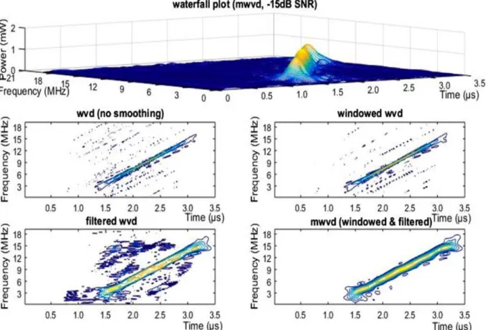
aforementioned forms of WVDs was carried out on MATLAB, and a graphical plot of the linear FM radar signal is shown in Fig. 1. The top part of the figure shows a three dimensional (3D) waterfall plot of power, time and frequency while the remaining parts show a two-dimensional (2D) contour plot of time and frequency of the same radar signal at an SNR of -15dB. The plot focuses on the first part out of four parts of the signal involving the PW aspect as this contains the required illustrations on the effect of the various WVDs. The signal was generated at center frequency of 2MHz to 17MHz, sampling frequency of 40MHz, PW of 2μs and PRP of 100μs
(generated delay of 1.25μs (50 samples)) for
illustration purpose. The center frequency follows the linear FM law based on the aforementioned theory and as such is presented in a range format while the PW is made higher in order to cater for this running frequency. It can be seen that the mWVD eliminates all forms of interferences and smoothens out the rough edges to some high level of degree due to its hybridization of the windowed and filtered WVD based on the aforementioned steps undertook in its design.
After the development of the mWVD, instantaneous powers (IP, Pi(t)) were obtained
in order to obtain the signal’s basic time parameters (PW and PRP) as the first steps of indentifying the signal. Three common ways of getting the IP in time-frequency analysis were considered. Firstly through tracing of the maximum power of the mWVD along the frequency axis (IPm) [23], secondly through summing of the power of the mWVD along the frequency axis also known as time marginal (IPtm) [20] and thirdly by conventional means of multiplying the signal with its complex conjugate (IPd) [25]. These are mathematically given in (8) – (10).
IPm = Pi,m(t) = max (pz,m(t, f)) (8)
IPtm = Pi,tm(t) = ∫ pz,m(t, f)df
∞
−∞ (9)
IPd = Pi,d(t) = |z(t)|2= z(t) ∗ z∗(t) (10)
where z∗(t) is the complex conjugate of z(t).
Thereafter, alternate form of these IPs were obtained by its smoothing via convolution operation using hamming window 0.5μs.
these alternate forms is expected to smoothen out the rough edges that will be present due to the effect of noise and the use of approximation methods. Finally, a precise algorithm was designed to measure the all PW and PRP at a selected desired threshold by interconnecting sub-functions of desired objective. The PW is simply the time for which IP samples is higher than the selected threshold. The PRP is the time for which IP samples is lower than the threshold plus the PW.
Performance analysis was carried out in the presence of additive white Gaussian noise (AWGN) at different range of SNR in order to test capability of the algorithm developed for the prediction of PW and PRP of a radar signal. The estimation criterion for this parameters was based on probability correct estimation (PCE) given in percentage. The test Linear FM radar signal’s PW of 4μs was selected to cater
for the FM law of the signal [14], while PRP of 100μs was used to model medium range
airborne radar [26]. A sampling frequency of 40MHz based on current radar technologies and bandwidth of 18MHz running from minimum frequency of 2MHz to maximum frequency of 20MHz to avoid aliasing was used. The signal contain standard set of four PWs and PRPs, i.e. total length of four PRP with some delay at the beginning to model normally captured radar signal [2]. However, it is the average of estimated time parameter that is connected to each SNR, where for every SNR, the PWs and PRPs were estimated ten times.
3.Results and Discussion
Three thresholds (25%, 37.5%, and 50%) in line with conventional practices [1] were used to estimate either the PW or PRP based on the methods discussed in the previous section. It is also important to point out the suffix use of –ns and –s to differentiate between the non-smooth and smooth versions of IPs considered in this paper respectively. The result obtained for PW estimation of the test radar signal at 25% threshold (Fig. 2).
It is observed (Fig. 2) that four out of the six methods considered in this paper achieved 100% PCE at different SNRs within the range of -8 dB to -4 dB. The four methods are the two versions of the IPd and the IPtm while the two versions of the IPm never achieve constant 100% PCE. This is attributed to the low threshold of 25% and its interaction with the underlying principle of the IP method. The best method at this threshold for PW estimation is the IPd-s with minimum SNR of -8 dB followed closely by other three remaining methods. This achievement by IPd-s iIPd-s attributed to the IPd-simplicity of itIPd-s formula as given in (10) when compared to the other methods. Result of Fig. 2 indicates that only one out of two methods gotten from mWVD is suitable for determining PW of the LFM signal at this threshold. The result derived for PW estimation of the test radar signal at higher threshold of 37.5% is given in Fig. 3.
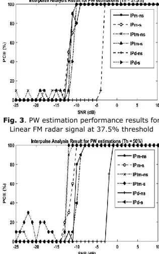
An improvement is noticed in Fig. 3 for 37.5% threshold when compared to Figure 2 of 25% threshold due to two main reasons. Firstly, all methods considered achieve constant 100% PCE at various SNRs as compared to four out of six methods of the result in Fig. 2. Secondly, the minimum SNR for 100% PCE is at a lower value of -10dB when compared to -8dB of the previous result of Fig. 2 and hence registering an improvement of 2dB.
Fig. 2. PW estimation performance results for Linear FM radar signal at 25% threshold
This minimum SNR is achieved by four methods; smooth versions of IPd and IPtm and ns versions of the IPm and IPtm. This indicates that sometimes, the smooth versions may not necessarily outperform the non-smooth versions. The two remaining methods; IPm-s and IPd-ns achieve 100% constant PCE at SNR difference of 1dB and 7dB respectively. The result deduced for PW estimation of the test radar signal at 50% threshold is given in Fig. 4.
The result obtained in Fig. 4 is similar to that of Fig. 3 considering all methods used in this paper also achieve 100% PCE at different SNRs. In some methods such as IPm-s, IPtm-ns and IPtm-s, improvements are observed as 100% PCE is achieved at slightly lower SNR when compared to those of 37.5% threshold in Fig. 3. However, in the other three remaining methods, higher minimum SNR is required to achieve 100% constant PCE when compared to same method of Fig. 3 of 37.5% threshold. Generally speaking, results obtained at 25% threshold of Fig. 2 shows 100% PCE in some methods at higher minimum SNR. This indicates the threshold of 37.5% and 50% being a better threshold choice for PW estimation of the linear FM radar signal.
It can be generally observed that PW can be estimated using the methods utilized in this work. This is because almost all methods achieve 100% PCE for all thresholds selected. The exception is that of the approximation method using IP obtained from the TFD maxima at a threshold of 25%. This is due to combination of the low threshold and approximation method. Also the best result obtained (at SNR of -12dB) is associated with IPtm followed closely by the IPd and then the IPm (no 100% PCE at threshold of 25%) when the smooth versions of the method used are considered. It is also observed that smooth versions generally perform better than the non-smooth versions, and hence justifying the smoothing process. Another point is also that the most versatile method is shared between IPtm and IPd methods with the IPtm slightly coming top. It has a better SNR at threshold of 50% with difference of 4dB, constant at 37.5%, and poorer at 25% with difference of 3dB. The result realized for the PRP estimations of the test radar signal at 25% threshold first just like those PW estimations is given in Fig. 5.
It is observed that all methods considered for this threshold in Figure 5 achieved 100% PCE at different SNRs. A major observation is the obtainment of same minimum SNR for both versions (s and ns version) of the approximate IP method gotten from the mWVD. This minimum SNR is -10 dB and -9 dB for the IPm and IPtm respectively. This is attributed to the combination of the linear nature of the test signal and high samples of PRP duration of the radar signal. However the advantage of smoothing is noticed in the IPd
method where the smooth version
outperforms the non-smooth version with SNR difference of 4dB. A higher threshold of 37.5% for the estimation of this same time parameter and the result obtained is given in Fig. 6.
Fig. 3. PW estimation performance results for Linear FM radar signal at 37.5% threshold
Fig. 4. PW estimation performance results for Linear FM radar signal at 50% threshold
Fig. 5. PRP estimation performance results for Linear FM radar signal at 25% threshold
.
Similarity in results obtained in Figure 5 is observed in Fig. 6 where all techniques achieved 100% PCE at various SNR. In fact, the same SNR of -10 dB is observed for both versions of the IPm in PRP estimation of Figure 6 just like that of Fig. 5. This indicates the independence of PRP estimation on the two thresholds when the IPm method is used. However, for IPtm, slightly lower SNR is required for 100% constant PCE with difference of 1dB and 2dB for the smooth and non-smooth versions obtained. Therefore, IPtm records a better PRP estimation with higher threshold. Lastly for the IPd; the non-smooth version requires higher SNR with difference of 1dB while the smooth version requires lower SNR with difference of 2dB. Generally speaking, the IPtm-s is found to be the best approach for PRP estimation of the test signal at threshold of 37.5% with minimum SNR of -11 dB to achieve 100% constant PCE. The result realized for the PRP estimations of the test radar signal at 50% threshold is shown in Fig. 7.
Table 1 Comparison of different time parameter estimation techniques
Method Minimum
SNR Time-marginal instantaneous
power (Present research) -1dB
Filters and Fast Fourier
transform [10] 4dB
Smoothed Instantaneous
Energy [13] 5dB
Short time Fourier transform
[11] 9dB
Auto-Convolution/Peak
Estimates [9] 20dB
All methods considered in this paper achieves 100% PCE at different SNR as shown in Fig. 7 just like those in Figs. 5 and 6. However, the similarity in minimum SNR for 100% PCE observed in previous PRP estimation results of Fig. 6 and Fig. 7 is not
noticed here. The smooth versions
outperform the non-smooth ones with a difference of 2dB, 1dB and 7dB observed for IPm, IPtm and IPd respectively. This is attributed to the higher threshold of 50% when compared to the others of 25% and 37.5%. Similarly a much higher difference is noticed for IP gotten directly (IPd) when compared to the other approximate methods (IPm and IPtm) due to underlying theory of the formulas presented in (8) – (10). The best method for this threshold remains IPtm-s just like that of 37.5% threshold of Fig. 6.
Generally observation on the PRP estimation at different thresholds shows the PRP estimations performing better than the PW estimations for this type of radar signal considering the fact that all methods used achieved 100% PCE at various SNRs due to its larger samples [27]. Also, the smooth versions perform better than the non-smooth versions in the majority of the PRP estimation cases. However, a key point of note is that the PRP estimations follow very closely (or the same in most cases) the result obtained with that of the PW estimations for this signal with path followed to achieve this being different. This is attributed to the fact that PW of the linear FM test signal is higher than those possible for other type of radar signal such as the simple pulsed and the phase shift keying ones. This attribution allows the PW results in effect start to mimic the results obtained for those PRP estimations [13]. In-line with convention, the method used in this work represented by worst possible result at 100% PCE is compared with previous work of similar objectives as shown in Table 1.
Fig. 6. PRP estimation performance results for Linear FM radar signal at 37.5% threshold
Fig. 7. PRP estimation performance results for Linear FM radar signal at 50% threshold
It is seen from Table 1 that methods used in this paper outperform previous works. This is due to the fact that PW and PRP can be estimated even at the level of higher noise power when compared to others. These results obtained from IP approximate methods henceforth allow forming the basic classifier able to separate LPI signals from non-LPI signals. This is because LPI signals always have higher PWs in order to allow enough time for the pulse compression modulation.
4.Conclusion
Heuristic steps taken to form a modified WVD were presented, where a combination of DI and LI kernel filter is used for the modification. Graphical interpretation is presented by comparison of all the WVDs; normal WVD, windowed WVD, filter WVD and the modified WVD. Furthermore, first application of determining the radar capabilities by estimating the PW and PRP is carried out by further time-frequency analysis involving the obtainment of various forms on instantaneous powers. The objective of comparing different IP methods for obtaining PW and PRP estimation was achieved based on the presented results and discussion. This is because almost all methods considered achieved 100% PCE at different SNR for these estimations. Also, the IP obtained through time-marginal of TFD outshines the other methods at any selected threshold with a minimum SNR of -5dB. Furthermore, it was observed that the smooth versions performed better than non-smooth version with SNR difference of 0dB to as much as 7dB noted. Finally, the PW results followed closely those of the PRP despite the difference in value due to its high samples.
Conflict of Interests
The authors declare that there is no conflict of interests regarding the publication of this paper.
References
[1] R. G. Wiley, ELINT: the interception and
analysis of radar signals. Boston: Artech House,
2006.
[2] M. Skolnik, Radar handbook, 3rd ed. Chicago: McGrawHill Companies, 2008.
[3] L. Weihong, Z. Yongshun, Z. Guo, L. Hongbin, “A method for angle estimation using pulse width of target echo,” In Proc. International Conference on Wireless Communications & Signal Processing, November 13 – 15, 2009, Nanjing: China, pp. 1-5.
[4] Y. Liu, Q. Zhang, “Improved method for deinterleaving radar signals and estimating PRI values,” IET Radar Sonar Nav, vol. 12, no. 5, pp. 506-514, 2018.
[5] J. Matuszewski, “The radar signature in recognition system database,” In Proc. 19th International Conference on Microwave Radar and Wireless Communications, May 21 – 23, 2012, Warsaw: Poland. pp. 617-622.
[6] K. I. Nishiguchi, M. Kobayashi, “Improved algorithm for estimating pulse repetition intervals.” IEEE Trans. Aerosp. Electron. Syst.,
vol. 36, no. 2, pp. 407-421, 2000.
[7] Y.-H. Quan, Y.-J. Wu, Y.-C. Li, G.-C. Sun, M.-D. Xing, “Range-Doppler reconstruction for frequency agile and PRF-jittering radar.” IET
Radar Sonar Nav, vol. 12, no. 3, pp. 348-352,
2018.
[8] P. Sedivy, “Radar PRF staggering and agility control maximizing overall blind speed,” In Proc. Conference on Microwave Techniques, April 16-18, 2013, Pardubice: Czech Republic. pp. 197-200.
[9] Y. Chan, B. Lee, R. Inkol, F. Chan, “Estimation of Pulse Parameters by Convolution,” In Proc. Canadian Conference on Electrical and Computer Engineering, May 7 – 10, 2006, Ottawa: Canada. pp. 17-20.
[10] W. Pei, T. Bin, “Detection and estimation of non-cooperative uniform pulse position modulated radar signals at low SNR,” In Proc. International Conference on Communications, Circuits and Systems, November 15 -17, 2013, Chengdu: China. pp. 214-217.
[11] A. A. Ahmad, A. Z. Sha'ameri, “Classification of airborne radar signals based on pulse feature estimation using time-frequency analysis,”
Defence S&T Technical Bulletin, vol. 8, no. 2,
pp. 103-120, 2015.
[12] A. A. Ahmad, A. Daniyan, D. O. Gabriel, “Selection of window for inter-pulse analysis of simple pulsed radar signal using the short time Fourier transform,” Int. J. Eng. Technol., vol. 4, no. 4, pp. 531-537, 2015.
[13] A. Adam, B. Adegboye, I. Ademoh, “Inter-pulse analysis of airborne radar signals using smoothed instantaneous energy,” Int. J. Signal
Process Syst., vol. 4, no. 2, pp. 139-143, 2016.
[14] P. E. Pace, Detecting and Classifying Low
Probability of Intercept Radar. Norwood: Artech
House, 2009.
[15] N. Levanon, E. Mozeson, Radar Signals. New Jersey: John Wiley & Sons, 2004.
[16] M. A. Richards, Fundamentals of Radar Signal
Processing. New York: McGraw-Hill Education,
2005.
[17] S. Hu, X. Wang, Q. Si, “Effects of FM linearity of linear FM signals on pulse-compression performance,” In Proc. International Conference on Radar, October 16 – 19, 2006, Shanghai: China. pp. 1-5.
[18] M. A. Govoni, H. Li, J. A. Kosinski, “Range-doppler resolution of the linear-FM noise radar waveform.” IEEE Trans. Aerosp. Electron. Syst,
[19] C. Baylis, J. Martin, M. Moldovan, R. J. Marks, L. Cohen, J. de Graaf, et al. “Spectrum analysis considerations for radar chirp waveform spectral compliance measurements,” IEEE T.
Electromagn. C., vol. 56, no. 3, pp. 520-529,
2014.
[20] J. Ville, Theory and applications of the notion of complex signal, translated by I. Seline in RAND
Tech. Rpt, Santa Monica, CA, 92. 1958.
[21] E. Wigner, “On the quantum correction for thermodynamic equilibrium,” Physical Review,
vol. 40, no.5, pp. 749-755, 1932.
[22] A. A. Ahmad, A. Saliu, A. E. Airoboman, U. Mahmud, S. Abdullahi, “Identification of radar signals based on time-frequency agility using
short-time Fourier transform.” J. Adv. Sci. Eng.,
vol. 1, no.2, pp. 1-8, 2018.
[23] B. Boashash, Time-frequency signal analysis
and processing: a comprehensive reference.
London: Academic Press, 2016.
[24] K. Prabhu, Window functions and their
applications in signal processing. Florida: CRC
press, 2013.
[25] A. Antoniou, Digital Signal Processing. Toronto: McGraw-Hill, 2006.
[26] G. Stimson, Introduction to Airborne Radar. New Jersey: SciTech Pub, 1998.
[27] J. G. Proakis, D. G. Manolakis, Digital Signal
Processing: Principles, Algorithms, and
Applications, New Jersey: Prentice Hall, 1996.