Multi-task learning in Computer Vision

(1)

MSc thesis

Master’s Programme in Computer Science

Multi-task learning in Computer Vision

Konsta Kutvonen

May 31, 2020

Faculty of Science

University of Helsinki

(2)

Associate Professor Laura Ruotsalainen

Examiner(s)

Associate Professor Laura Ruotsalainen, Professor Jyrki Kivinen

Contact information

P. O. Box 68 (Pietari Kalmin katu 5) 00014 University of Helsinki,Finland

Email address: [email protected] URL: http://www.cs.helsinki.fi/

(3)

Faculty of Science Master’s Programme in Computer Science

Konsta Kutvonen

Multi-task learning in Computer Vision

Associate Professor Laura Ruotsalainen

MSc thesis May 31, 2020 67 pages

computer vision, deep learning, convolutional neural networks, multi-task learning

Helsinki University Library

Algorithms study track

With modern computer vision algorithms, it is possible to solve many different kinds of prob-lems, such as object detection, image classification, and image segmentation. In some cases, like in the case of a camera-based self-driving car, the task can’t yet be adequately solved as a direct mapping from image to action with a single model. In such situations, we need more complex systems that can solve multiple computer vision tasks to understand the environment and act based on it for acceptable results. Training each task on their own can be expensive in terms of storage required for all weights and especially for the inference time as the output of several large models is needed. Fortunately, many state-of-the-art solutions to these problems use Con-volutional Neural Networks and often feature some ImageNet backbone in their architecture. With multi-task learning, we can combine some of the tasks into a single model, sharing the convolutional weights in the network. Sharing the weights allows for training smaller models that produce outputs faster and require less computational resources, which is essential, espe-cially when the models are run on embedded devices with constrained computation capability and no ability to rely on the cloud.

In this thesis, we will present some state-of-the-art models to solve image classification and object detection problems. We will define multi-task learning, how we can train multi-task models, and take a look at various multi-task models and how they exhibit the benefits of multi-task learning. Finally, to evaluate how training multi-task models changes the basic training paradigm and to find what issues arise, we will train multiple multi-task models. The models will mainly focus on image classification and object detection using various data sets. They will combine multiple tasks into a single model, and we will observe the impact of training the tasks in a multi-task setting.

ACM Computing Classification System (CCS)

Computing methodologies→Artificial intelligence→Computer vision

Computing methodologies→Machine learning→Learning paradigms→Multi-task learning

HELSINGIN YLIOPISTO – HELSINGFORS UNIVERSITET – UNIVERSITY OF HELSINKI Tiedekunta — Fakultet — Faculty Koulutusohjelma — Utbildningsprogram — Study programme

Tekij¨a — F¨orfattare — Author

Ty¨on nimi — Arbetets titel — Title

Ohjaajat — Handledare — Supervisors

Työn laji — Arbetets art — Level Aika — Datum — Month and year Sivumäärä — Sidoantal — Number of pages

Tiivistelm¨a — Referat — Abstract

Avainsanat — Nyckelord — Keywords

Säilytyspaikka — Förvaringsställe — Where deposited

(4)

(5)

1 Introduction

Since 2012 computer vision research has been increasingly dominated by approaches using deep Convolutional Neural Networks (CNNs). These CNN based techniques have allowed for achieving significantly better results in computational image and video understanding compared to previous state-of-the-art approaches. Nowadays, there are many interesting avenues of computer vision research, such as image segmentation, object detection, object recognition, image captioning, pose detection, and many more. Since the task of computa-tional image understanding is quite complex, the CNNs used to solve these problems often require dozens, if not hundreds of millions of parameters, in order to achieve sufficiently reliable accuracies. As the number of parameters is high, the networks require large com-putational resources to find optimal values for all of the variables in all of the hundreds of layers of matrices. Graphics Processing Units (GPUs) or Tensor Processing Units (TPUs) are the tools that people use to train the parameters in the networks since the training operations are highly parallelizable, allowing for the training of networks with hundreds or even thousands of layers. The problem often is that when training, one wants to increase the batch size, but at the same time, the computations must fit in the memory of the processing unit, which can be difficult to increase. Also, as the number of parameters in the model increases, the memory required for training the networks, and the time to produce outputs increases. To combat these problems, we often have to get better or more hardware, which can be expensive or compromise in the size of the model, which may lead to unreliable performance.

Embedded devices can use these CNN based algorithms to analyze their surroundings in an environment where they can’t rely on external predictions from the cloud. One of the most significant issues is that achieving scene understanding requires multiple classifiers to solve various tasks. For example, a camera-based self-driving car has numerous things it is interested in resolving using the video output of its cameras. The tasks could be, for example, finding and classifying other vehicles, traffic signs, road markings, predicting paths of vehicles, pedestrians, and other actors, understanding where it can move, and finally deciding the steering angle and acceleration for the car with the information. All these tasks have to be solved using the limited computing capability onboard the actor, and the inference time for them can’t be too long in order to react to everything within a reasonable time frame. Here we have many tasks, and if every task requires its independent

(8)

network to produce the outputs, and we cut down on the network sizes, the classifiers might be powerful enough to produce safe outputs. On the other hand, if we don’t reduce the network sizes, our inference time might be too long for a real-time system. One way to possibly get a good compromise between inference time and model complexity is to use multi-task learning and weight sharing within the model to get a single model with multiple outputs and similar or better performance to individual classifiers.

Multi-task learning proposes some solutions to these problems but makes the training process more difficult. Still, in some cases, it is something that has to be done to get a good enough inference time and accuracy on the problem at hand. Many modern computer vision models already feature an ImageNet backbone as a part of the classifier, so this is a good part of the network to consider for sharing. However, finding which tasks and how much can be shared is a difficult problem to solve.

1.1 Scope of study

In this thesis, we will present state-of-the-art solutions to fundamental computer vision problems, like image classification and object detection. We will present the architectures of these models and show how the ImageNet backbones are an essential part of solving these problems. Using the presented solutions, we will make use of various data sets to train multi-task models and evaluate the effects of training multi-task models.

1.2 Structure of thesis

Chapter 2 will present some basic terminology for describing convolutional neural networks that will be used throughout the thesis. We won’t cover the very basics of neural networks or the exact inner workings of convolutional neural networks, and refer to (Goodfellow et al., 2016) for studying those details.

Chapter 3 covers the modern image classification models, describing their architecture and how to train them. We will also describe why the ImageNet is such a valuable data set to so many problems. We will demonstrate the significance of the ImageNet models by defining transfer learning and describing how it is instrumental in solving small-scale problems with the ImageNet models as backbones.

(9)

3

computer vision problems. Multi-task learning is also a useful technique in other domains of machine learning, but we focus only on computer vision. We will define multi-task learning and see how it relates to transfer learning. Also, the basic differences of multi-task training to a single-multi-task setting are described, and some examples of multi-multi-task models are shown. Finally, the theoretical benefits and issues that may arise are talked about and demonstrated using some examples.

Chapter 5 describes what object detection is and how to evaluate object detection models. We will also briefly discuss the basic parts of an object detector and the difference between single and two-stage object detectors. Finally, we will cover the EfficientDet architecture in detail and explain how to train an object detector by using it.

In chapter 6, we will cover the results of our experiments on training multi-task models. The first experiment is about training image classifiers on plant imagery. The second experiment is about training multi-label classifiers. The third experiment covers training object detectors with multiple datasets. The fourth experiment uses a single EfficientDet to do image segmentation and object detection. Finally, we will summarize our experiences in training multi-task models and explain what problems we encountered.

(10)

2 Neural networks

The topics presented in this thesis are based on neural networks, especially convolutional neural networks, which are a distinct neural network variation for image processing using filters. Here we provide a very brief high-level overview of some of the concepts that are important for the later chapters, but a more detailed overview of deep learning and neural networks can be found, for example, in (Goodfellow et al., 2016).

2.1 Convolutional Neural Networks

The most significant component of Convolutional Neural Networks (CNNs) is the convo-lutional layers that are their primary building block. Using convoconvo-lutional filters allows neural networks to extract useful information from images to accomplish various tasks. The convolutional blocks are based on the mathematical convolution operation of captur-ing the signal of pre-determined window size. A CNN classifier often consists of multiple convolutional layers with other layers in between. Successive convolutional layers build on top of one another, and the deeper layers get high activations on more specific features. In many final models, the earlier layers are thus somewhat similar and re-usable as they often detect relatively primitive shapes, like diagonal or horizontal lines. In this thesis, we often talk about the parameters or the weights of a network. The number of parameters in a network tells how complex it is and how expensive it is to store. The floating-point numbers in the various layers are these weights, which are generally 32-bit numbers, but their precision can vary.

2.1.1 Parameters

To get the total number of parameters required for a single convolutional layer, we need to determine the input size, convolution window size, and the number of filters. For example, if the input is a 256x256 RGB image, the input size is 256x256x3. Now, if we apply 16 filters with a window size of 5, each of the filters requires 5x5x3 parameters, bringing the total to 1200 parameters. A fully connected layer with 1000 hidden units would require a matrix with around 200 million parameters, so it would not really be possible even to

(11)

5

apply multiple of these layers while maintaining the image size. The convolution allows for keeping the dimensions between successive layers and only modifying the number of channels between the layers. Often convolutional models reduce the first two dimensions, and the number of channels increases in the deeper layers. For this, the convolutions can use a stride parameter to skip some positions for the convolution. The pooling layer is another way to reduce the size. Generally used pooling layers are average and maximum pool layers. They are applied similarly to a convolution but capture the average or the maximum of a window. Neither of these approaches requires any extra learnable weights.

2.1.2 Embedding

Generally, the role of the convolutional layers in a CNN model is to act as a feature extractor. As can be seen in the number of parameters of the fully connected layer on a full-sized image, the image needs to have a smaller dense representation in order to connect a linear layer to it. This representation can be generated with the convolutional layers. The final representation that can be pushed into a linear classifier for some final inference is called an image embedding. Embeddings are representations of things in relatively small continuous numbered vectors, here we consider embeddings of images, but embeddings are used, for example, for words and sentences as well. Besides just doing classification, the embeddings can represent things, for example, faces or objects. When a general embedding is generated it can be used to for example to evaluate if someone is the same person as the embedding or to find similar images.

2.1.3 Backbone

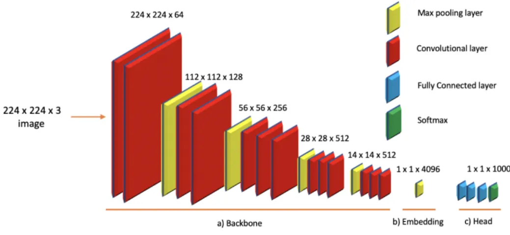
The feature extraction part of a convolutional classifier is called the backbone. The back-bone is annotated in Figure 2.1. Finding better features is often correlated with more parameters and a larger model, but various architectural decisions can also help. The largest convolutional models have thousands of layers. Best models often use as large backbones as is possible within the constraints of the specific deployment. The backbone is thus responsible for creating the image embedding that is used to produce an output. Some tasks require feature maps taken from the middle of the backbone instead of only relying on the final layer.

(12)

Figure 2.1: Image of an example of a convolutional neural network architecture with backbone (a), image classifier (b) and task head (c) labeled. The architecture in this image is the VGGNet (Simonyan and Zisserman, 2015).

2.1.4 Head

The final layers of a classifier are called the head. The head is responsible for producing the output, and its exact architecture varies from task to task. It could be just a single linear layer connecting the image embedding to final class probability distribution or an image segmentation model classifying each pixel in the image. The head can thus contain whatever layers are needed to get the output, combining batch normalization, dropout, convolutional, recurrent, and linear layers depending on what is needed to solve the task. An example visualization of how the different parts of a convolutional model are connected is shown in Figure 2.1. The architecture would vary on a task-by-task basis, and the figure shows a basic image classifier architecture.

(13)

3 Image classification

Image classification is one of the essential modern computer vision problems, where the goal is to create a model that can classify an input image into one of a set of pre-defined classes. Before the popularization of applying large Convolutional Neural Networks for this task, the most successful way of solving the problem was to use some algorithm for finding feature descriptors in a set of images to construct a Visual Bag of Words (Faheema and Rakshit, 2010). A linear classifier, like a Support Vector Machine, would then do the classification using the Bag of Words representation of an image. These days nearly all approaches are based on using deep CNNs, and working CNNs were deployed already in 1998 on character recognition in the form of LeNet (LeCun et al., 1998). In this chapter, we will present what ImageNet (Deng et al., 2009) is and how the models trained with it are important when applying transfer learning, and we will show an example of how it can be done.

3.1 ImageNet

ImageNet (Deng et al., 2009) has been one of the most significant data sets for image classification. It is has enabled the development and served as a benchmark for several significant improvements to modern computer vision techniques. The ImageNet challenge (ImageNet Large Scale Visual Recognition Competition (ILSVRC) 2020) is a competition consisting of a selected collection of 1000 classes and a total of 1.2 million training images and 150 thousand test images from the ImageNet data set. Winning models from the ImageNet competition have provided some of the essential architectures modern computer vision algorithms use. In 2012 the winning model, AlexNet (Krizhevsky et al., 2017), showed that it was possible to train deep CNNs efficiently using GPUs. Since 2012 all top-performing models showed some new improvements on how to create the most performant network architecture, for example, VGGNet (Simonyan and Zisserman, 2015) from the year 2014 and ResNet (He, X. Zhang, et al., 2016) from 2015, both of which have been popular models to use for Transfer Learning since.

Human accuracy in image classification on the ImageNet challenge is about 5.1% (Rus-sakovsky et al., 2015), ResNet achieves a top-5 error rate of 3.57% (He, X. Zhang, et al.,

(14)

2016) and newer architectures even lower, but this still does not mean that image clas-sification is a solved problem. The human performance experiment found that many of the human errors are caused by not having expert information in, for example, identifying animal species or not even being aware of the existence of a class (Russakovsky et al., 2015). ObjectNet (Barbu et al., 2019) is a dataset designed to test image classifiers with a focus on their generalizability. It contains many classes that also exist in the ImageNet dataset. However, the objects in the images are in unexpected locations or have an unex-pected pose, causing the high accuracy image classifiers trained on ImageNet to experience a 40-45% accuracy drop when evaluating them on the ObjectNet images of classes shared between ImageNet and ObjectNet. This kind of adjustment is relatively easy for a human, and it shows that while the classifiers are good, they are by no means perfect.

3.2 Transfer learning

Transfer learning is a powerful technique to obtain results quickly when using deep CNNs. Here we will only take a look at transfer learning within the domain of deep CNNs, but it is a technique that has been successfully applied to many other domains of machine learning as well.

The idea behind transfer learning is to train on a task that would produce useful features in solving some other task. Then the network weights in the model for the actual task are initialized to those of the model we are transferring from, so the training of the original model is a pre-step to the real task. Since training the models on ImageNet scale datasets is not generally feasible due to their large number of parameters and long training time, one of the pre-trained models is picked and then fine-tuned. Fine-tuning a classifier means that some existing model is used as a weight initializer, and the network is then trained on the data of another task, updating the weights of the original classifier to better align with the new task. The transfer learning approach differs significantly from the traditional learning model, where each task requires a separate model that learns from the given data using random weights. Since image inputs are often very high dimensional, the traditional approach may not work in many cases. The pre-training allows for focusing on data that provides answers to the actual task and not on learning low-level features, which the ImageNet classifiers would already have learned.

To give a formal definition of transfer learning, we will follow the definitions provided in (Pan and Yang, 2010). Let D be a domain, which consists of a feature space X and a

(15)

9

marginal probability distribution P(X). For a given domain, a task T T ={Y, f(X)}

consists of a label spaceY for the inputs and of a predictive functionf(x) which produces predictions for all pairs {xi, yi} where xi ∈ X and yi ∈ Y. Given a source domain DS,

a source task TS, a target domain DT and a target task TT, where target and source are

disjoint, transfer learning tries to improve the performance offT(x) usingDS and TS.

Unlike the ImageNet challenge, most real-world tasks do not have such an abundance of data for all possible classes. Still, to achieve the highest accuracies, they require models that are equal in terms of complexity to those that have top accuracies problems on the scale of the ImageNet classification. For this reason, many CNN classifiers, irrespective of the problem, feature one of the ImageNet classifiers in the model architecture. Even though some datasets may contain a large number of images per class, using a pre-trained classifier as a basis often produces a better final classifier by applying fine-tuning (Kornblith et al., 2019).

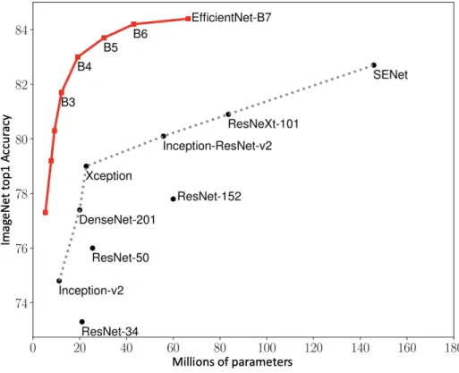
Figure 3.1: Number of parameters in popular ImageNet classifiers. Figure adapted from (Tan and Le, 2019).

Picking which classifier to use as a base is often problem-dependent. As it is not possible to declare one network structure to be the best at all tasks, picking the best model to

(16)

start with usually requires the user to compare different architectures and weighing the requirements for the problem at hand. Often though, the larger models will perform better, and there exists a correlation between performing well on ImageNet and being a good transfer learning model (Kornblith et al., 2019). Though as can be seen in figure 3.1, better performance often comes at the cost of many more parameters, requiring more memory to train the model. Though, as the results in (Lee et al., 2020) show, just the number of parameters is not the only thing to compare as the throughput of a Resnet50 turns out to be about three times as large as the throughput of an EfficientNet-B4 (Tan and Le, 2019) even though they have a similar amount of parameters. So in the case of time-constrained inference environments, also the time required for an inference has to be taken into account when picking models. Often though, the number of parameters is a relatively good proxy for the inference time. The throughput is likely due to the differences in the internal implementations of the EfficientNet and normal CNNs.

If there is enough data, it turns out that using a pre-trained network does not provide any benefits in terms of the converged model accuracy, but it is not detrimental to performance either (He, Girshick, et al., 2019). When training sufficiently long on a sufficient amount of data, the pre-trained and randomly initialized networks converged to similar accuracies but required significantly different amounts of training resources. Still, this does not mean that pre-training is useless by any means as the saved resources and getting models to converge faster are essential factors for progress. And of course, there is not enough data in many cases, and training from scratch will not provide satisfying results due to the large number of parameters that would need to be optimized. In these cases, it would then be a decision to apply transfer learning or to get a model that is not good enough to produce reliable results.

3.3 ResNet

ResNet is one of the first effective and very deep Convolutional Neural Network architec-ture that was presented in 2015 and won the ImageNet challenge. Prior to the publication of ResNet, the most powerful networks were relatively shallow, like VGGNet (Simonyan and Zisserman, 2015), which has only 19 layers. One of the big issues relating to training deep networks is vanishing gradients, where gradients disappear when they are backprop-agated through many layers (Zagoruyko and Komodakis, 2016). ResNets utilize residual connections around bottleneck building blocks, which allow for the networks to contain

(17)

11

many more layers than those without them, the largest network presented in the original ResNet paper was 152 layers, totaling for around 8x increase in the number of layers when compared to earlier networks (He, X. Zhang, et al., 2016).

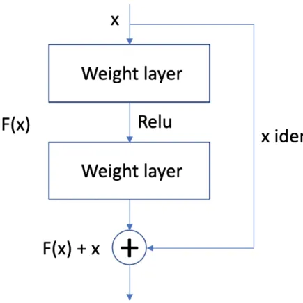
Figure 3.2: Resnet building block for learning the residual (He, X. Zhang, et al., 2016)

The ResNet block architecture allows for the blocks to learn the identity function more efficiently by trying to learn the residual function instead of the direct mapping. The residual can be learned by adding the unchanged weights of an earlier layer to the output of some transformations on it. The residual block is shown in Figure 3.2. Normally a neural network layer learns the mapping between x and y using a function H(x), but by the same token, we can learn a residual transformation. Learning these residuals using the identity mapping skip-connections is the revolutionary idea introduced by the ResNet. Since these skip-connections are only connections and not extra layers, they do not require extra parameters that would need to be learned. The residual transformation is

(18)

where H is the mapping of two or more network layers. Both of these approaches should approximate the same functions; the difference is in how easy it is for the network to learn. Learning a transformation of F(x) = 0 would intuitively seem easier for a neural network than learningF(x) =x. As can be seen from the success of the ResNets compared to non-residual networks, this is what allows for creating very deep networks. If the transformation changes the input size, a matrix W is necessary to map the input to the same dimensions, generating the final formula for a residual block.

y=F(x,{Wi}) +Wsx

where Wi and Ws are the the weight matrices to be applied to x.

Many variants of ResNet exists, such as wide ResNets (Zagoruyko and Komodakis, 2016), ResNeXt (Xie et al., 2017) and others. Also the DenseNet (G. Huang et al., 2017) is heavily inspired by ResNets. ResNet-50, ResNet-34, ResNet-101, and ResNet-152 are still some of the most popular models to use when a pre-trained ImageNet trained backbone is needed for some part of a classifier as they produce good results and do not contain too many parameters compared to some other architectures.

3.4 Improving model performance

Improving model performance is not easy, but using the various types of skip-connections, such as the ones used in ResNet residual blocks with the identity transform, it is possible to increase the size of the network to massive sizes. A 557 million parameter model called GPipe (Y. Huang et al., 2019) takes the model scaling to the extreme and requires some unique parallelism libraries to train the model. It is still only slightly better than previous models, showing that size is not the only thing that matters.

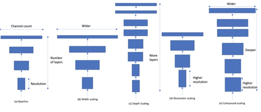
There are three main ways to scale up a network, as shown in figure 3.3. Scaling by depth means adding more layers to the model, allowing for more complex dependencies to be captured by the model. For example, ResNet-1000 is a very deep type of ResNet, but it has similar performance to a ResNet-101, so there are diminishing returns when trying to scale up by depth (Tan and Le, 2019). Scaling by width means increasing the number of channels in the layers, and it is especially popular when optimizing smaller size models, such as MobileNet (Howard et al., 2017). Wide ResNets (Zagoruyko and Komodakis, 2016) increase the width of the ResNet blocks and allow for better features and easier training. The third way is to increase the resolution of the input. A higher resolution

(19)

13

Figure 3.3: Various ways of scaling network architectures (Tan and Le, 2019). a) Shows the baseline network. b) Shows how to scale by the number of channels. c) Shows how to scale the number of layers. d) Shows how to scale by resolution. e) Shows how to scale all the metrics with a compound factor.

allows for the network to find more specific features as the level of detail increases, and often specific network architectures work best at one particular resolution.

The other approach to finding a better architecture is to use different kinds of blocks that are better. One way of finding better building blocks is by manual experimentation. The other, like in the case of MnasNet (Tan, Chen, et al., 2019), is to pose the problem as an optimization problem and to use Neural Architecture Search (Elsken et al., 2019) to find the optimal solution. In the case of MnasNet, the goal is to maximize the model architecture m in

ACC(m)×[LAT(m)

T ] w

whereT is the target, by searching in a constrained space. So the goal is to optimize the accuracy (ACC) of the model with a given latency (LAT) on a specific device. The search produces small but very efficient models when the target device is a mobile phone.

3.5 EfficientNet

EfficientNet models form a family of models ranging from EfficientNet0 to EfficientNet7 that were generated by smartly scaling existing convolutional models to optimize them for efficiency in a similar way to MnasNet (Tan and Le, 2019). The more complex models are created by using compound scaling on the EfficientNet0 model, shown in Figure 3.3 (e), where the width, depth, and the resolution of the network are scaled using a factor φ. As the cost of neural architecture search grows exponentially as the size of the network grows,

(20)

the search is only done on the base model. The search of φ is a constrained optimization problem, where width, depth and, resolution are constrained such that dφ×wφ×rφ ≈2 and each increase in φ increases network FLOPS by 2φ_{. The architecture search for the}

base network is similar to that of MnasNet. The target of EfficinetNet is to maximize the model m

ACC(m)×[F LOP S(m)

T ]

w

so the goal is to optimize for both accuracy (ACC) and number of floating-point operations (FLOPS) instead of latency as in MnasNet (Tan and Le, 2019).

As seen in figure 3.1, these optimizations allow for the EfficientNet to form a very per-formant architecture using a low amount of parameters that does well on ImageNet and is good at Transfer Learning also. Interestingly though, the reduction in FLOPS and pa-rameters do not directly translate to low real-world inference time. As is compared in the paper, an EfficientNet-B1 gets a 5.7x speedup over a ResNet-152, while the EfficientNet scores significantly higher on ImageNet. So in terms of the time and accuracy ratio, the EfficientNet seems to do well. When looking at the inference time in terms of FLOPS and parameters, we can find out that the ResNet would be more efficient, as the ResNet has 7.6x as many parameters and 16x FLOPS when compared to the EfficientNet, but the inference time multiplier is 5.7x. From this comparison, we can easily see that the number of FLOPS is not a direct proxy for inference time. Instead, the optimization should be for latency directly as in MnasNet if that is the goal.

The proposed EfficientNet models use mobile inverted bottleneck (MBConv) blocks used in MobileNetV2 (Sandler et al., 2018) in constructing the base model. The MobileNet uses a Depthwise Separable Convolution, where a depthwise convolution and a pointwise convolution are applied in sequence. The depthwise convolution applies di kxk filters to

the input, where di is the input channels and k is the kernel size leading to an output channel count dj =di. A normal convolutional layer would apply multiple filters having M channels with the computational cost ofhiwididjk2, whereas the depthwise convolution

only has a cost of hiwidi(k2+dj), reducing the cost by k2. The result of the depthwise

convolution then runs through a pointwise convolution, where a 1×1×dj 1d convolution

is applied to get the final output as a linear combination of the channels. The inverted residuals in MBConv are connections similar to ResNet, but in this case, they are connected between the low dimensional layers.

(21)

15

3.6 Training image classifiers

An image classifier’s basic function is to predict which of some set of classes exists in an image. So, to train a model to answer such a question, a data set with images and accompanying labels are needed. For example, the Oxford-IIT Pets dataset (Parkhi et al., 2012) consists of images of 37 different cat and dog species and labels for those images signifying which of the 37 classes an image represents. The dataset consists of about 200 images per class, so it is relatively small and an excellent example of a situation where transfer learning is instrumental in getting good results.

After the data of the images and labels are gathered to a data loader, that outputs small batches for training, the model needs to be constructed. For the backbone, any ImageNet classifier will do. For example, EfficientNet-B4 could be a good decision. So we will initialize the backbone of our model with the weights of a pre-trained EfficientNet that was trained on the ImageNet data set by someone with access to large computational resources. After the model has been initialized, the head has to be changed to be compatible with our new task. By default, the model will be expecting to classify images to the thousand classes of the ImageNet. In this case, we want to solve the 37 cat and dog species problem, so the final fully connected layer has to be changed. It will be initialized as a fully connected layer with 37 output units, representing each of the classes, connecting the embedding to the outputs. The head does not need to be just a single, fully connected layer, but it could also contain more fully connected layers, dropout layers, and batch normalization layers and more. Adding more than a single fully connected layer might be a good idea if the backbone remains frozen and is not fine-tuned. That way, the head can learn some useful combinations of the image embedding instead of optimizing the features in the backbone. Once all the layers are in place, the model needs to be optimized with a training loop. Every iteration, a loss needs to be calculated for the batch that has been sampled from the data loader. To be able to calculate the loss, the outputs of the final fully connected layer need to be normalized into a distribution of probabilities with softmax. The softmax is defined as

Sof tmax(xi) =

exp(xi)

P

jexp(xj)

For each classi, there is an output score ofxi, for which we will calculate the proportion of

its score with respect to the sum of all the classes’ scoresxj, creating the probability

dis-tribution. Since we have a single correct class, we would want to maximize the probability of the correct class and minimize the probability of the other classes. The loss function to

(22)

do exactly this optimization is called categorical cross-entropy, and it is defined as follows. CE =−1 N N X i=1 (yi∗log(pi) + (1−yi)∗log(1−pi))

Where N is the number of classes, yi is either 1 or 0 depending on if it is the correct label

and pi is the probability for that class. This formula does exactly what we previously

described that we wanted to do. To get the loss for a single class, if y = 1, the value will be the first part of the sum, if y = 0, the value will be the second part of the sum, since (1−yi) is now 1. When we optimize the model, in the case of the chosen architecture, the

(23)

4 Multi-task learning

Multi-task learning is a generalization of Transfer Learning to training a single model where the goal is to optimize for multiple objectives. Training a multi-task model requires a set of distinct tasks to be posed as a multi-task learning problem. It can have many benefits when applied correctly, such as making the models more general by regularization and reducing computational requirements. On the other hand, if multi-task learning is applied to problems that don’t train well in a multi-task setting, the resulting models can be significantly worse than the single-task counterparts. Here we look at examples of multi-task learning in computer vision. Especially recently, with the introduction of transformers like BERT (Devlin et al., 2019), multi-task learning and transfer learning have gained popularity within natural language processing, but to restrict our scope, we only consider how to apply multi-task learning in computer vision.

4.1 Definition

Multi-task learning is quite similar to transfer learning. However, the main difference lies in the fact that the goal is to generalize to solve and improve performance in all tasks using some shared representation. In contrast, transfer learning aims to optimize a single new task, ignoring the performance on the original task entirely. Often in multi-task learning, the shared layers are initialized using some ImageNet model and transfer learning as the ImageNet backbone is an architectural feature shared in many models.

The formal definition for multi-task learning follows the definition given in (Y. Zhang and Yang, 2018). A learning problem consists of m related learning tasks {Ti}mi=1 that are

trained together. Each task has a dataset Di with ni pairs {xij, yji} ni

j=1, where xij refers

to the input of task Ti and y_ji is the label corresponding to the input vector. Let Xi = (xi

1, ..., xini) be the input matrix for taskTi. In a multi-task setting there can bexsuch that

x∈Xi _and _x_∈_Xj _or_Xi ₌_Xj _{for some} _i₆₌_j_{, meaning that a single image has multiple}

labels or an entire data set has labels for multiple tasks.

To train the network, each task Ti needs to have its loss function defined. A commonly used way to get the total loss of the input is by using the weighted loss functions for all

(24)

tasks, resulting in a formula

Ltotal=X

i wiLi

, whereLi is the loss function for taskTi and wi, is the weight that specifies the sensitivity

of the task (Cipolla et al., 2018). The sensitivity multiplies the loss of the task. Multiplying the loss has the effect of making the error on the task with higher sensitivity to have a larger impact on the adjustment of weights. So the sensitivity should be used to either pick tasks that are important or to normalize the losses if they are very different. There can be significant differences in the scale of the losses if different tasks use different loss functions. The sensitivity of the tasks is an essential parameter to get right as choosing a too high parameter for some task might lead to a solution that is optimal for only the most sensitive task, starving the others (Standley et al., 2019).

Once the loss function is specified, the actual training is quite similar to training a single-task model. The one new thing to consider in a multi-single-task setting is the sampling ratio of the different tasks as some tasks can be easier to learn or contain significantly more or less data compared to other tasks. Like in regular training, the models are trained one batch at a time. In a multi-task setting, we have datasets for each of the tasks from which we can pick at a time. Now, we can define an epoch e in the training process as the total number of batches from all tasks. The epoch can be formalized as

e =X

i

|Xi|αi Bi

batches over i tasks, where |Xi| is the training set size, Bi is the batch size, and αi is

the scaling factor for each task, telling how important the specific task is for the learning process. The sampling ratio is one of the new parameters that is required when doing multi-task learning on multiple datasets. When training models, some value has to be picked for the sampling ratios, and picking wrong values leads to worse models. Precisely what is a good sampling ratio is complicated to tell beforehand, and generally, the chosen values need to be evaluated by experimentation. Iterating through all batches can be done in a round-robin fashion, by going through all batches of each data set at a time or randomly sampling the sets with probabilities respective to their magnitude and scaling factor.

(25)

19

4.2 Latent image representations

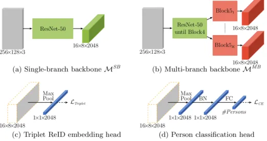
For a multi-task model, the optimal situation is such, where all classifiers would use a single shared latent representation of the image to predict all attributes. This representation is an image embedding, that would capture all valuable information of the image for our tasks. The embedding could be the vector represented by the final layer of an ImageNet classifier flattened to some n-dimensional vector that then solves all the tasks instead of just a single task. However, such a universal image representation can be challenging or

Figure 4.1: Example of partly and completely shared backbones. Figure from (Pfeiffer et al., 2019).

impossible to learn, and instead, only a part of the network is shared between the tasks. Here, this shared structure is called the backbone of the multi-task classifier. Often the backbone is in the form of some ImageNet classifier architecture, and it can be the entire classifier or some layers up to some arbitrary limit. As the amount of layers shared is picked for each task separately, some tasks can share the entire classifier as a backbone, and others might only share some amount of layer that produces desirable results.

Besides just deciding the network branching, each task requires an independent head that outputs prediction for that task. These task heads are similar to those used in transfer learning, where only a single task is solved using the ImageNet backbone. Especially in a multi-task setting, these heads can be more than just a single linear layer calculating the softmax over all classes. A single head can contain any combination of several linear layers, dropout layers, batch normalization layers, convolutional layers, or it could be a Recurrent Neural Network creating a caption for the image embedding, depending on the

(26)

task at hand. In Figure 4.1, we can see an example of the flexibility of the sharing as the model can use a completely shared backbone or a branching backbone, which has a unique head for each task, solving the person re-identification and classification tasks.

4.3 Benefits

Depending on how and where multi-task learning is applied, it can provide a multitude of benefits to the model. Many of these benefits stem from the fact that the model gets to see more data, and the various tasks can make it easier to find useful features. Different kinds of data sets have different kinds of noise, learning multiple tasks makes it easier to distinguish which features are beneficial and detrimental some features may be difficult to learn on a dataset but can be useful and borrowed from another and learning multiple tasks forces the model to not overfit on one of them (Ruder, 2017).

These benefits come up when the tasks are compatible and allow the model to learn more general features, generally leading to better performance on the distinct tasks. When the needed features between tasks are conflicting, the model performance tends to go down (Kokkinos, 2017). The problem of deciding what to share is not easy to solve.

The benefits of multi-task learning come up, especially when dealing with limited amounts of data, in which case, particularly finding the features that matter without overfitting can be complicated. For example (W. Zhang et al., 2020) found that multi-task learning could improve gene expression pattern classifiers when trained in a multi-task setting. The multi-task classifier was significantly better than the one only using transfer learning, showing that the features learned were more general.

Another significant boon of multi-task models, especially in embedded domains, is the reduction in model size and inference time. As many classifiers are dependent on an embedding of an image to produce results, using a shared embedding of an image for multiple tasks means that the model requires only a single partly or completely shared backbone. For example (Kocabas et al., 2018) uses a shared backbone to detect people in an image and to detect keypoints on their body and then finally to do a semantic segmentation of the image while also improving performance on most of the tasks. Finally, a model using multi-task learning can take advantage of the different losses to produce a more optimal loss weighing strategy compared to constant weighting. Picking the weights in the total loss function is very important as with invalid weights, the

(27)

op-21

timization can be difficult or even impossible (Gong et al., 2019). The weights become even more critical if the losses for various tasks are different, for example, one task might use mean squared error as a loss function and another cross-entropy, and the resulting loss values might differ by orders of magnitude. The total loss function can be modified by adding an uncertainty weighting to each of the tasks by considering the uncertainty of the prediction (Cipolla et al., 2018). Depending on the task, the benefit compared to an unweighted loss can be significant (Cipolla et al., 2018) or, in some cases, only small (Gong et al., 2019).

4.4 Hard parameter sharing

A hard parameter sharing setting is one where the same convolutional weights in the in-termediate layers solve multiple tasks, like in Figure 4.1. Hard parameter sharing is the primary way of reducing total model size and inference time when solving multiple tasks simultaneously. While sharing the weights can provide many benefits to the end model, as seen in the previous chapter, it comes at the cost of an increased number of tunable parameters when training the models. As we have previously seen, multi-task models in-troduce new constant factors to the training process beyond the normal hyperparameters for learning rate, dropout rate, and others. These include the hyperparameters for weigh-ing the loss functions and determinweigh-ing the task samplweigh-ing ratios, but also the expensive to evaluate architectural decision of which tasks should share representations and how much should be shared.

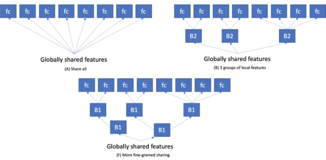
In Figure 4.2, there are multiple ways of configuring a multi-task network in terms of what to share. The results for the different configurations were quite varied. However, even the worst multi-task Model A did better on every task when compared to the single-task models, and accuracy improvement from the single-single-task case to the best multi-single-task Model F was roughly 20% (Park et al., 2019). These results are quite validating for the presumed benefits of multi-task models. Since these results show that it is possible to share the majority of the network parameters and, at the same time, increase the performance, even with the most greedy share-all model. Though, at the same time, it shows that multiple compute-expensive experiments have to done to find the most optimal sharing structure for the backbone network.

In the experiments done by (Park et al., 2019), they utilized auxiliary training to great effect. They had two original features of interest that were sugar and alcohol level in the

(28)

Figure 4.2: Some ways of sharing features between tasks. Here the global features are from resnet. The fc blocks are fully-connected heads. B1 is one ResNet block and B2 is two ResNet blocks. Out of these model F was the best. Figure adapted from (Park et al., 2019).

drinks. Other features were added as auxiliary training features to improve the perfor-mance on the two original features (Park et al., 2019). This auxiliary training can also be done by, for example, using ImageNet to keep the original classifier accurate on ImageNet while training on the new data set like in (W. Zhang et al., 2020); this way, the model won’t be able to overfit on the new data so easily. In the drink classification experiment, the auxiliary tasks were picked in a way that they might help in finding the correct features to solve the actual tasks (Park et al., 2019). Adding auxiliary tasks is an interesting way of forcing features into the model that the developer thinks could be useful for the model to find, in that sense, they are hand-crafted features that get augmented in the model. In practice, this means that if we are training a model e.g., to predict the steering angle given an image, we might want to add an auxiliary task that predicts the lane markers to make it easier to learn these features as they should be a significant feature for producing correct outputs.

A similar multi-task model in (Pfeiffer et al., 2019), also partly visualized in Figure 4.1, solves 6 different tasks in a single model. The tasks in that model are very different from one another, including person re-identification, pose estimation, and image segmentation. The interesting result in their search for related tasks is that while a pair of tasks don’t work well together, they can work well when combined with other tasks. For example, they found that just pairing the pose estimation head with other tasks significantly reduces

(29)

23

its accuracy, but when all tasks use the single shared backbone, it does just as well as if trained in a single-task setting. These results show that very different tasks can combine to a single model to provide a very significant reduction in model size while producing about as good or better accuracies.

4.5 Soft parameter sharing

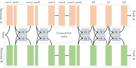
Figure 4.3: Cross-stitch architecture. Figure from (Misra et al., 2016).

Soft parameter sharing is quite similar to learning each task on its own since each task has separate weights. Soft parameter sharing happens by picking some layers, where some metrics constrain the parameters to be similar, likel2 distance (Ruder, 2017).

The sharing functionality can be more complicated than just basic regularization. For example, the Cross-stitch units (Misra et al., 2016) are a particular type of soft sharing, where the stitch units combine tasks A and B using a linear combination of the activations, visualized in Figure 4.3. The benefit here is that the user does not need to specify how much should be shared between the tasks, but it is instead learned in the cross-stitch unit. If nothing needs to be shared, then the network can learn to assign the weight for the other task to zero.

This kind of sharing does not scale very well as the number of tasks increases since cal-culating the relation between various tasks is quadratic. Since the joining logic requires extra parameters, it means there is even more to learn than just learning all the tasks separately. As soft sharing does not provide many of the benefits that are gained by hard

(30)

sharing the parameters, it is not as popular. However, it is useful in adding some extra information between the tasks to gain extra performance by utilizing the latent represen-tations between them in various ways. Also, in the basic case of using a soft parameter share to constraint, the layers can improve the generalizability of the model.

4.6 Attention augmented Multi-task learning

In a multi-task setting, the model ends up having a representation of the image from each task’s point of view, and it is possible to use attention (Vaswani et al., 2017) to augment the predictions. Especially in the case where the tasks are heavily correlated, this can be quite useful. For example, when doing weather recognition, it would make sense that some of the features are correlated, and this correlation can be used by adding an attention layer between the different tasks, like in (Zhao et al., 2019). The Multi-Task Attention Network (MTAN) (Liu, Johns, et al., 2019) is an example of a more advanced application of attention in multi-task models. In the MTAN, each task gets its own attention module, and they are used to determine correlations of the tasks at specific layers of the network using the attention operations. It is similar to cross-stitching networks in that each task has to learn its attention module features. However, there is only a single backbone for the shared features, and the attention modules are responsible for producing the task level outputs. The number of parameters is still significantly reduced as the task specific-parts are not complete ImageNet classifiers, resulting in a significantly more efficient and accurate classifier for image segmentation.

4.7 What and when to share

What makes or breaks a multi-task model is the decision on what should be shared, but determining what and how much should be shared is exponentially more expensive as the number of tasks grows. Currently, there is no definitive way of theoretically evaluating which tasks should have a shared representation and just how much can be shared. As experimentation is expensive, a good starting point is to try to find similar tasks that should do well together. However, there is no guarantee that even all the tasks within a single family of problems are beneficial for joint training, so some experimentation has to be done. The desired result in a multi-task setting would be to share all the parameters between all the tasks, but as can be seen in (Kokkinos, 2017), that approach often

(31)

signif-25

icantly reduces performance. If sharing an entire network does not produce good results, it can be a good idea only to share some part of it as the lower level features tend to be more general (Oquab et al., 2014). By sharing only a part of the network, it may be possible to strike the right balance between performance and model complexity.

Figure 4.4: The taskonomy task similarity tree. Figure from (Zamir et al., 2018).

An attempt to create a taxonomy of related tasks called Taskonomy to find out what tasks are beneficial for transfer learning exists in (Zamir et al., 2018). The Taskonomy experiments pre-trained networks on tasks and then evaluated whether the features would transfer well to other tasks to end up with a hierarchical categorization of related tasks, shown in Figure 4.4. Still, the authors noted that, depending on model architecture and data set, the results could be different.

It would make sense that the results of the Taskonomy would be easily transferable to the multi-task setting. When evaluating the multi-task vs. transfer affinity, it turns out that they are negatively correlated, at least in the case of the five tasks that were the focus of the experiments in (Standley et al., 2019). Based on this observation, it can be beneficial to train some non-related tasks together. The authors suggest that the different tasks act as a good form of regularization as the models need to generalize to multiple types of inputs. It could also be that some of the learned features work very well for the other task, but can’t be easily learned with the dataset of the other task and vice versa. These results are aligned with the empirical results that we saw when we looked at the compatibility of classifiers using hard weight sharing. Currently, it seems not to be possible to determine the compatibility of different tasks purely on a theoretical grounding. Instead, experiments need to be run, and the results of pairs of tasks do not always generalize to a set of all other tasks when using shared representations in models (Pfeiffer et al., 2019).

(32)

5 Object detection

Object detection is another prevalent task in the domain of computer vision. An object detection task is one where the goal is to localize one or many different classes of objects using bounding boxes. Before current deep learning-based techniques, a popular way to solve the problem was to use handcrafted features like in image classification and to use a sliding window over the image for localizing objects. These previous techniques include, for example, the Viola-Jones detector (Viola and Jones, 2001), which uses a sliding window and AdaBoost for features, and another popular method was using histograms of oriented gradients (Dalal and Triggs, 2005) to find where the boundaries of objects exist. These days there exist various ways of using the feature maps of neural networks for learning the filters to get much better results. The various architectures can be split into two approaches, one-stage detectors, and two-stage detectors. The two-stage detectors require region proposals, based on which the object detection is done. An often-used family of these kinds of methods is the R-CNN classifiers, for example, the faster R-CNN (Ren et al., 2015). In the one-stage detectors, features from various layers of the classifier are used to get the predictions. For example, the YOLOv4 (Bochkovskiy et al., 2020) is the 4th iteration of the single-stage YOLO family of detectors that are very popular due to the good balance between fast speed and good accuracy.

(33)

27

5.1 Metrics

The training of object detection models requires data sets that have been labeled for that purpose. Generally, the data sets contain bounding box annotations for each of the classes in the data set, such as seen in Figure 5.1. For this reason, object detection models can’t use a simple metric like the basic accuracy in image classification. As the images are often manually labeled, the boxes are most likely not completely consistent. So most likely, the predictions are never going to align with the labeled boxes perfectly. Consequently, the method for evaluating object detection performance is Average Precision (AP) or mean Average Precision (mAP) or one of their variants. These metrics use intersection over union (IoU) score to evaluate how incorrect the predicted bounding box is when compared to the actual label. Intersection over union is visualized in Figure 5.2.

Figure 5.2: The visual formula for calculating intersection over union.

To get to a final AP score, the first thing that has to be decided is the IoU score threshold for considering a prediction to be correct. For example, we could consider all predictions

(34)

that have over 50% or 75% overlap in the IoU. The threshold value for IoU that should be used is not entirely standardized, and there are multiple ways of calculating the AP score. For example, the popular COCO dataset (T.-Y. Lin, Maire, et al., 2014) uses an average of 10 IoU scores ranging from .5 to .95 IoU thresholds as the main metric. To get the AP for a class, we need to graph the precision-recall curve and then calculate the area under it. For example, the Pascal Visual Object Classes Challenge (VOC) (Everingham et al., 2010) recommends doing this by using 11 points of interpolated precision. So we get the following formula for Average Precision:

AP = 1 11

X

r∈{0,0.1,...,0.9,1}

pinterp(r)

Where pinterp is defined as

pinterp(r) = max

˜

r:˜r≥rp(˜r)

Then to get the mAP score, we can average the AP score for each of the classes in the data set. As was mentioned, this way of calculating the AP is not always the same, for example, the COCO metrics (COCO - Common Objects in Context 2020) recommend using 101 points for integrating the curve instead of the 11 proposed in the VOC. This discrepancy in the integration means that not all AP scores are directly comparable.

5.2 Object detection model structure

Much like image classifiers and many other vision tasks, modern object detectors rely on pre-trained backbones to generate the features required for predicting bounding boxes. A classifier head is required to get these predictions, but in object detectors, this head is more complicated than in image classification.

For the backbone, most object detection architectures use one of the same ImageNet models as in image classification such as ResNet or VGG. However, the YOLO models use DarkNet, which is specifically designed for achieving efficient results in object detection (Bochkovskiy et al., 2020). The main reason for picking one backbone over another is often a function of both accuracy and inference time. As object detectors are often run on video data, inference time can be more significant than in image classification, as it is often desirable to be able to run them in real-time.

(35)

29

The head is where the architectures differ the most, and generally, any backbone could be combined with a specific detector head. The head comprises of a neck, which connects the intermediate features from the backbone to the final head. The intermediate features are generally connections from some specific layers of the backbone. Earlier single-stage detectors used the extracted features directly, but the current state-of-the-art methods use special feature pyramids and path aggregation to get the best results (Tan, Pang, et al., 2020). For example, the YOLO v4 uses spatial pyramid pooling (He, X. Zhang, et al., 2015) over the DarkNet features and path aggregation net (PANet) (Liu, Qi, et al., 2018) to concatenate the parameters for the classifier head (Bochkovskiy et al., 2020). Different ways of combining the feature pyramids are described in Figure 5.3. Like many other parts of the architecture, picking one is a trade-off of more parameters and inference time and accuracy.

Figure 5.3: a) Basic FPN (T.-Y. Lin, Doll´ar, et al., 2017) where features are combined in only one direction. b) PANet modifies the basic FPN by adding a path from the lower level features to higher-level features. c) BiFPN tries to prune the connections to the most important ones. Image adapted from (Tan, Pang, et al., 2020).

In two-stage detectors like faster R-CNN (Ren et al., 2015), there is a region proposal network (RPN), which predicts region proposals using a sliding window for some anchor boxes. Running this RPN is expensive, and often the two-stage models are much slower

(36)

than the single-stage detectors. The benefit of the two-stage approach is generally a better accuracy. Still, recently the one-stage methods like YOLO v4 have achieved very similar accuracies to the two-stage ones with much faster inference times (Bochkovskiy et al., 2020). By utilizing new ways of using the feature maps, the object detectors have recently become significantly better over the years, as can be seen from the different iterations of the YOLO models, as they have been using very similar backbones over the years (Bochkovskiy et al., 2020).

5.3 Multi-dataset training

Often an object detection problem requires detecting multiple different classes in a similar context. For example, a self-driving car would need to detect various traffic signs, cars, pedestrians, road markings, cyclists, and many other things. Collecting a single dataset that has labels for all of the classes of interest can be a very daunting task. Even if it is feasible to create the dataset for the original classes of interest, this approach does not scale very well when new classes need to be recognized. As likely the original dataset might contain millions of images labeled for multiple classes, adding a new class would require going through the entire dataset again and labeling the new class as well. The new class may be relatively rare; for example, we may be interested in detecting emergency vehicles with sirens on. Here is where multi-dataset learning is highly beneficial as it only allows for collecting a specific class dataset. This type of cross-dataset learning is useful when we need to combine multiple distinct data sources to detect some union of the labels (Yao et al., 2020).

The main difficulty in combining multiple datasets for detection lies in the fact that they likely contain unlabeled overlapping classes. For example, given a dataset for detecting cars and another for detecting stop signs, we have two distinct datasets where only one of the classes is labeled. If we train this model, assuming that the labels are genuinely valid, we will end up unlearning the tasks due to the overlap of the classes. The problem lies in the fact that it is most likely that in the car dataset, we will find stop signs that are not labeled. Similarily we will find cars that are unlabeled within the stop sign dataset. When we naively train this model, we will end up detecting cars and stop signs that are actually correct but incorrect based on the labels. The model will be punished for detecting these non-labeled positive examples due to the absence of the labels.

(37)

31

loss. For example, in (Yao et al., 2020), the RetinaNet (T. Lin et al., 2017) model’s loss function is modified to ignore the losses for tasks that are not a part of the dataset. All models using the same focal loss as RetinaNet can be trained with this adjusted loss function. This way, each class will get its own positive and negative dataset to train on and not affect the performance of the other classes. Still, this does not completely solve the problem as some of the classes might require conflicting features, as can be the case when very different tasks are combined. In that case, it could be smart to split the similar classes into different detectors and maybe share only the lower levels between all tasks. Similar multi-dataset training can also be applied in multi-label image classification set-tings. A multi-label image classification problem is one where we want to assign multiple labels to an image. For example, we might want to classify whether it is raining, the sun is shining, the sea is visible, is there a dog in the image, and so on for all the classes of interest. Again, collecting a dataset containing all labels for all images is quite expensive, but we can train this with a separate binary classification head for each task. And as collecting a separate dataset for each task is relatively easy, it is possible to create a quite powerful model with relative ease.

5.4 EfficientDet

EfficientDet (Tan, Pang, et al., 2020) is an object detection model, that is based on the previously covered EfficientNet ImageNet model. The neck for the EfficientDet is a unique bidirectional feature pyramid network (BiFPN). The EfficientDet model also uses similar compound scaling as the EfficientNet models for the new object detection specific parts. The scaling factor is used for the BiFPN network, box and class predictor networks, and to find the optimal input resolution. The EfficinetDet shows that improving the backbone is quite useful for the entirety of the model. This can especially be seen when looking at the comparisons of using a ResNet vs an EfficientNet as the backbone in the same EfficientDet architecture (Tan, Pang, et al., 2020). The EfficientDet model architecture is shown in Figure 5.4.

The different feature maps in the BiFPN are combined using a weighted feature fusion. The feature maps can’t be directly combined since they have different dimensionality, so they have to be up or downsampled depending on the direction of the connection. By weighing each feature map, the network can learn how important each feature map is. Since the dimensionalities differ from one another, they likely don’t contribute equally to

(38)

Figure 5.4: EfficientDet architecture comprises of the EfficientNet (Tan and Le, 2019) backbone, the bidirectional feature pyramid network neck and the class and box classifier heads. Here only one BiFPN layer is pictured, but there are multiple of them normally stacked in succession.

the output feature maps, which is signified by the learned weight. The BiFPN connection architecture is a simplified version of the PANet, as shown in Figure 5.3. The goal of the changes from PANet is to have a more high-level fusion of features while dropping the nodes that have little feature fusion and then to stack multiple of these layers to get the final model (Tan, Pang, et al., 2020).

The efficient scaling of the parameters and the BiFPN architecture allow EfficientDet to produce impressive results at relatively high framerates. The new YOLO v4 produces very similar scores at acceptable framerates also (Bochkovskiy et al., 2020). Still, some slightly better results are produced by the two-stage detectors, but those can’t reach a 30 FPS inference time (Bochkovskiy et al., 2020). So in practice, using either the EfficientNet or YOLO is a good idea when video needs to be classified. The EfficientNet scales relatively well with larger EfficientNet backbones, but it is not possible to classify real-time video. This flexibility allows for picking the model with a suitable accuracy for the problem at

Multi-task learning in Computer Vision

MSc thesis

Master’s Programme in Computer Science