Differentiable Planners
Solving a RL Problem
Known reward,
known model.
Model-based RL
Model-free RL
with sparse
rewards
Better Optimization
Better Reward Signals
Convert into a
Supervised Training
Problem
Solve a Related but
Supervision-rich Problem
Build Models and Plan
with Them
Sim2Real
Structured
Policies
Structured Policies
Borrow policy structures from classical pipelines, and inject learning.
Typical Robotics Pipeline
Observations
Estimation
State
Planning
Control
6DOF Pose
Grasp Motion
Planning
Observed Images
Mapping
Planning
Observed Images
Path Plan
Geometric Reconstruction
Hartley and Zisserman. 2000. Multiple View Geometry in Computer Vision
Thrun, Burgard, Fox. 2005. Probabilistic Robotics
Canny. 1988. The complexity of robot motion planning. Kavraki et al. RA1996. Probabilistic roadmaps for path
planning in high-dimensional configuration spaces. Lavalle and Kuffner. 2000. Rapidly-exploring random
trees: Progress and prospects.
Video Credits: Mur-Artal et al., Palmieri et al.
Structured Policies
Borrow policy structures from classical pipelines, and inject learning.
Observations
State
Estimation
Planning
Control
If we can differentiate through the path planning step, we can train
state estimators, directly for outputting good control.
• Analytically differentiate through a planner
• eg: Differentiating through value iteration
• eg: Differentiating through MPC (this paper)
• Train a planner (and differentiate through it)
• eg: Value iteration networks
Value iteration networks
⇡modulated) valuesre(a| (s), (s)). The full network architecture is depicted in Figure 2 (left).(s). Finally, the vector (s) is added as additional features to a reactive policy Returning to our grid-world example, at a particular state s, the reactive policy only needs to query the values of the states neighboring s in order to select the correct action. Thus, the attention module in this case could return a (s) vector with a subset of V¯ ⇤ for these neighboring states.Figure 2: Planning-based NN models. Left: a general policy representation that adds value function features from a planner to a reactive policy. Right: VI module – a CNN representation of VI algorithm. Let ✓ denote all the parameters of the policy, namely, the parameters of fR, fP, and ⇡re, and note
that (s) is in fact a function of (s). Therefore, the policy can be written in the form ⇡✓(a| (s)), similarly to the standard policy form (cf. Section 2). If we could back-propagate through this function, then potentially we could train the policy using standard RL and IL algorithms, just like any other standard policy representation. While it is easy to design functions fR and fP that are differentiable (and we provide several examples in our experiments), back-propagating the gradient through the planning algorithm is not trivial. In the following, we propose a novel interpretation of an approximate VI algorithm as a particular form of a CNN. This allows us to conveniently treat the planning module as just another NN, and by back-propagating through it, we can train the whole policy end-to-end.
3.1 The VI Module
We now introduce the VI module – a NN that encodes a differentiable planning computation.
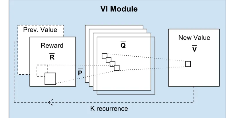
Our starting point is the VI algorithm (1). Our main observation is that each iteration of VI may be seen as passing the previous value function Vn and reward function R through a convolution layer and max-pooling layer. In this analogy, each channel in the convolution layer corresponds to the Q-function for a specific action, and convolution kernel weights correspond to the discounted transition probabilities. Thus by recurrently applying a convolution layer K times, K iterations of VI are effectively performed.
Following this idea, we propose the VI network module, as depicted in Figure 2B. The inputs to the VI module is a ‘reward image’ R¯ of dimensions l, m, n, where here, for the purpose of clarity, we follow the CNN formulation and explicitly assume that the state space S¯ maps to a 2-dimensional grid. However, our approach can be extended to general discrete state spaces, for example, a graph, as we report in the WikiNav experiment in Section 4.4. The reward is fed into a convolutional layer Q¯ with A¯ channels and a linear activation function, Q¯¯a,i0,j0 = Pl,i,j Wl,i,j¯a R¯l,i0 i,j0 j. Each channel
in this layer corresponds to Q¯(¯s, a¯) for a particular action ¯a. This layer is then max-pooled along the actions channel to produce the next-iteration value function layer V¯ , V¯i,j = maxa¯ Q¯(¯a, i, j). The next-iteration value function layer V¯ is then stacked with the reward R¯, and fed back into the convolutional layer and max-pooling layer K times, to perform K iterations of value iteration.
The VI module is simply a NN architecture that has the capability of performing an approximate VI computation. Nevertheless, representing VI in this form makes learning the MDP parameters and reward function natural – by backpropagating through the network, similarly to a standard CNN. VI modules can also be composed hierarchically, by treating the value of one VI module as additional input to another VI module. We further report on this idea in the supplementary material.
3.2 Value Iteration Networks
We now have all the ingredients for a differentiable planning-based policy, which we term a value iteration network (VIN). The VIN is based on the general planning-based policy defined above, with the VI module as the planning algorithm. In order to implement a VIN, one has to specify the state
4
Tamar et al. NeurIPS 2016. Value Iteration Networks
express value iteration computation as a convolutional network
(with max-pooling across channels)
Spatial Planning using Transformers
Open Review 2020. Differentiable Spatial Planning using Transformers link
long-range value prediction via transformers
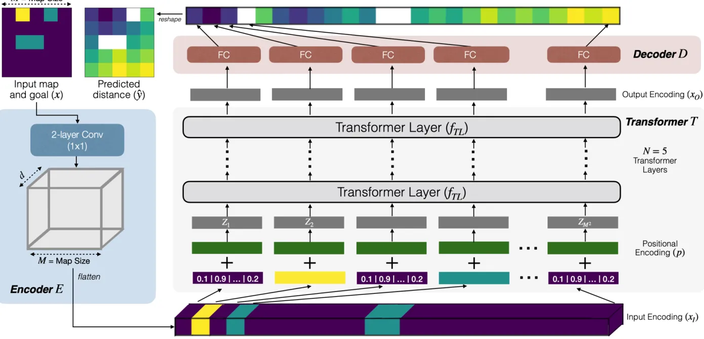
Under review as a conference paper at ICLR 2021Figure 3: Spatial Planning Transformer (SPT). Figure showing an overview of the proposed Spatial Planning Transformer model. It consists of 3 modules: an Encoder E to encode the input, a Transformer network T
responsible for planning, and a Decoder D decoding the output of the Transformer into action distances.
Both layers have a kernel size of 1 ⇥ 1, which ensures that the embedding of all the obstacles is
identical to each other, and the same holds true for free space and the goal location. The output of this convolutional network is of size d ⇥ M ⇥ M, where d is the embedding size. This output is then
flattened to get xI of size d ⇥ M2 and passed into the Transformer network.
Transformer. The Transformer network T converts the input encoding into the output encoding: xO = T(xI). It first adds the positional encoding to the input encoding. The positional encoding
enables the Transformer model to distinguish between the obstacles at different locations. We use a constant sinusoidal positional encoding (Vaswani et al., 2017):
p(2i,j) = sin(j/C2i/d), p(2i+1,j) = cos(j/C2i/d)
where p 2 Rd⇥M2 is the positional encoding, j 2 {1, 2, . . . , M2} is the position of the input, i 2 {1, 2, . . . , d/2}, and C = M2 is a constant.
The positional encoding of each element is added to their corresponding input encoding to get
Z = xI + p . Z is then passed through N = 5 identical Transformer layers (fTL) to get xO.
Decoder. The Decoder D computes the distance prediction yˆ from xO using a position-wise fully
connected layer:
ˆ
yi = WDTxT,i + bD
where xT,i 2 Rd⇥1 is the input at position i 2 1,2, . . . , M2, WD 2 Rd⇥1, bD 2 R are parameters
of the Decoder shared across all positions i and yˆi 2 R is the distance prediction at position i. The
distance prediction at all position are reshaped into a matrix to get the final prediction yˆ 2 RM,M.
The entire model is trained using pairs of input x and output y datapoints with mean-squared error as
the loss function.
3.2 END-TO-END MAPPING AND PLANNING
The SPT model described above is designed to predict action distances given a map as input. However, in many applications, the map of the environment is often not known. In such cases, an autonomous agent working in a realistic environment needs to predict the map from raw sensory observations. While it is possible to train a separate mapper model to predict maps from observations, this requires map annotations which are expensive to obtain and often inaccurate. In contrast, demonstration trajectories consisting of observations and optimal actions are more readily available or easier to obtain in many robotics applications. One of the key benefits of learning-based differentiable spatial planning is that it can be used to learn mapping just from action supervision in an end-to-end fashion without having access to ground-truth maps. To demonstrate this benefit, we train an end-to-end
Differentiable MPC for End-to-end Planning and Control
Brandon Amos1 Ivan Dario Jimenez Rodriguez2 Jacob Sacks2Byron Boots2 J. Zico Kolter13
1Carnegie Mellon University 2Georgia Tech 3Bosch Center for AI
Abstract
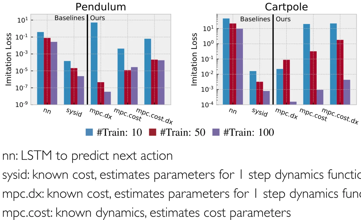
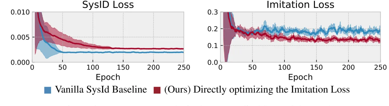
We present foundations for using Model Predictive Control (MPC) as a differen-tiable policy class for reinforcement learning in continuous state and action spaces. This provides one way of leveraging and combining the advantages of model-free and model-based approaches. Specifically, we differentiate through MPC by using the KKT conditions of the convex approximation at a fixed point of the controller. Using this strategy, we are able to learn the cost and dynamics of a controller via end-to-end learning. Our experiments focus on imitation learning in the pendulum and cartpole domains, where we learn the cost and dynamics terms of an MPC policy class. We show that our MPC policies are significantly more data-efficient than a generic neural network and that our method is superior to traditional system identification in a setting where the expert is unrealizable.
1 Introduction
Model-free reinforcement learning has achieved state-of-the-art results in many challenging domains. However, these methods learn black-box control policies and typically suffer from poor sample complexity and generalization. Alternatively, model-based approaches seek to model the environment the agent is interacting in. Many model-based approaches utilize Model Predictive Control (MPC) to perform complex control tasks [González et al., 2011, Lenz et al., 2015, Liniger et al., 2014, Kamel et al., 2015, Erez et al., 2012, Alexis et al., 2011, Bouffard et al., 2012, Neunert et al., 2016]. MPC leverages a predictive model of the controlled system and solves an optimization problem online in a receding horizon fashion to produce a sequence of control actions. Usually the first control action is applied to the system, after which the optimization problem is solved again for the next time step. Formally, MPC requires that at each time step we solve the optimization problem:
argmin x1:T2X,u1:T2U T X t=1 Ct(xt, ut) subject to xt+1 = f(xt, ut), x1 = xinit, (1)
where xt, ut are the state and control at time t, X and U are constraints on valid states and controls, Ct : X ⇥ U ! R is a (potentially time-varying) cost function, f : X ⇥ U ! X is a dynamics model,
and xinit is the initial state of the system. The optimization problem in eq. (1) can be efficiently
solved in many ways, for example with the finite-horizon iterative Linear Quadratic Regulator (iLQR) algorithm [Li and Todorov, 2004]. Although these techniques are widely used in control domains, much work in deep reinforcement learning or imitation learning opts instead to use a much simpler policy class such as a linear function or neural network. The advantages of these policy classes is that they are differentiable and the loss can be directly optimized with respect to them while it is typically not possible to do full end-to-end learning with model-based approaches.
In this paper, we consider the task of learning MPC-based policies in an end-to-end fashion, illustrated in fig. 1. That is, we treat MPC as a generic policy class u = ⇡(xinit; C, f) parameterized by some
representations of the cost C and dynamics model f. By differentiating through the optimization
problem, we can learn the costs and dynamics model to perform a desired task. This is in contrast to
32nd Conference on Neural Information Processing Systems (NeurIPS 2018), Montréal, Canada.
•
•
,
• Paper is about, how to compute gradient:
the value function by approximating the value iteration algorithm with convolutional layers. Karkus et al. [2017] connects a dynamics model to a planning algorithm and formulates the policy as a structured recurrent network. Silver et al. [2016] and Oh et al. [2017] perform multiple rollouts using an abstract dynamics model to predict the value function. A similar approach is taken by Weber et al. [2017] but directly predicts the next action and reward from rollouts of an explicit environment model. Farquhar et al. [2017] extends model-free approaches, such as DQN [Mnih et al., 2015] and A3C [Mnih et al., 2016], by planning with a tree-structured neural network to predict the cost-to-go. While these approaches have demonstrated impressive results in discrete state and action spaces, they
are not applicable to continuous control problems.
To tackle continuous state and action spaces, Pascanu et al. [2017] propose a neural architecture which uses an abstract environmental model to plan and is trained directly from an external task loss.
Pong et al. [2018] learn goal-conditioned value functions and use them to plan single or multiple steps of actions in an MPC fashion. Similarly, Pathak et al. [2018] train a goal-conditioned policy to perform rollouts in an abstract feature space but ground the policy with a loss term which corresponds to true dynamics data. The aforementioned approaches can be interpreted as a distilled optimal controller which does not separate components for the cost and dynamics. Taking this analogy further, another strategy is to differentiate through an optimal control algorithm itself. Okada et al. [2017] and Pereira et al. [2018] present a way to differentiate through path integral optimal control [Williams et al., 2016, 2017] and learn a planning policy end-to-end. Srinivas et al. [2018] shows how to embed differentiable planning (unrolled gradient descent over actions) within a goal-directed policy. In a similar vein, Tamar et al. [2017] differentiates through an iterative LQR (iLQR) solver [Li and Todorov, 2004, Xie et al., 2017, Tassa et al., 2014] to learn a cost-shaping term offline. This shaping term enables a shorter horizon controller to approximate the behavior of a solver with a longer horizon to save computation during runtime.
Contributions of our paper. All of these methods require differentiating through planning proce-dures by explicitly “unrolling” the optimization algorithm itself. While this is a reasonable strategy, it is both memory- and computationally-expensive and challenging when unrolling through many iterations because the time- and space-complexity of the backward pass grows linearly with the forward pass. In contrast, we address this issue by showing how to analytically differentiate through the fixed point of a nonlinear MPC solver. Specifically, we compute the derivatives of an iLQR solver with a single LQR step in the backward pass. This makes the learning process more computationally tractable while still allowing us to plan in continuous state and action spaces. Unlike model-free approaches, explicit cost and dynamics components can be extracted and analyzed on their own. Moreover, in contrast to pure model-based approaches, the dynamics model and cost function can be learned entirely end-to-end.
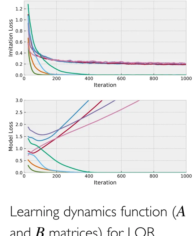
3 Differentiable LQR
Discrete-time finite-horizon LQR is a well-studied control method that optimizes a convex quadratic objective function with respect to affine state-transition dynamics from an initial system state xinit. Specifically, LQR finds the optimal nominal trajectory ⌧1:?T = {xt, ut}1:T by solving the optimization
problem ⌧1:?T = argmin ⌧1:T T X t=1 1 2 ⌧ > t Ct⌧t + c>t ⌧t subject to x1 = xinit, xt+1 = Ft⌧t + ft. (2)
From a policy learning perspective, this can be interpreted as a module with unknown parameters ✓ = {C, c, F, f}, which can be integrated into a larger end-to-end learning system. The learning process involves taking derivatives of some loss function `, which are then used to update the parameters. Instead of directly computing each of the individual gradients, we present an efficient way of computing the derivatives of the loss function with respect to the parameters
@` @✓ = @` @⌧1:?T @⌧1:?T @✓ . (3) 3
the value function by approximating the value iteration algorithm with convolutional layers.
Karkus
et al.
[
2017
] connects a dynamics model to a planning algorithm and formulates the policy as a
structured recurrent network.
Silver et al.
[
2016
] and
Oh et al.
[
2017
] perform multiple rollouts using
an abstract dynamics model to predict the value function. A similar approach is taken by
Weber
et al.
[
2017
] but directly predicts the next action and reward from rollouts of an explicit environment
model.
Farquhar et al.
[
2017
] extends model-free approaches, such as DQN [
Mnih et al.
,
2015
] and
A3C [
Mnih et al.
,
2016
], by planning with a tree-structured neural network to predict the cost-to-go.
While these approaches have demonstrated impressive results in discrete state and action spaces, they
are not applicable to continuous control problems.
To tackle continuous state and action spaces,
Pascanu et al.
[
2017
] propose a neural architecture
which uses an abstract environmental model to plan and is trained directly from an external task loss.
Pong et al.
[
2018
] learn goal-conditioned value functions and use them to plan single or multiple
steps of actions in an MPC fashion. Similarly,
Pathak et al.
[
2018
] train a goal-conditioned policy to
perform rollouts in an abstract feature space but ground the policy with a loss term which corresponds
to true dynamics data. The aforementioned approaches can be interpreted as a distilled optimal
controller which does not separate components for the cost and dynamics. Taking this analogy further,
another strategy is to differentiate through an optimal control algorithm itself.
Okada et al.
[
2017
]
and
Pereira et al.
[
2018
] present a way to differentiate through path integral optimal control [
Williams
et al.
,
2016
,
2017
] and learn a planning policy end-to-end.
Srinivas et al.
[
2018
] shows how to embed
differentiable planning (unrolled gradient descent over actions) within a goal-directed policy. In
a similar vein,
Tamar et al.
[
2017
] differentiates through an iterative LQR (iLQR) solver [
Li and
Todorov
,
2004
,
Xie et al.
,
2017
,
Tassa et al.
,
2014
] to learn a cost-shaping term offline. This shaping
term enables a shorter horizon controller to approximate the behavior of a solver with a longer horizon
to save computation during runtime.
Contributions of our paper.
All of these methods require differentiating through planning
proce-dures by explicitly “unrolling” the optimization algorithm itself. While this is a reasonable strategy,
it is both memory- and computationally-expensive and challenging when unrolling through many
iterations because the time- and space-complexity of the backward pass grows linearly with the
forward pass. In contrast, we address this issue by showing how to
analytically
differentiate through
the fixed point of a nonlinear MPC solver. Specifically, we compute the derivatives of an iLQR solver
with a
single
LQR step in the backward pass. This makes the learning process more computationally
tractable while still allowing us to plan in continuous state and action spaces. Unlike model-free
approaches, explicit cost and dynamics components can be extracted and analyzed on their own.
Moreover, in contrast to pure model-based approaches, the dynamics model and cost function can be
learned entirely end-to-end.
3 Differentiable LQR
Discrete-time finite-horizon LQR is a well-studied control method that optimizes a convex quadratic
objective function with respect to affine state-transition dynamics from an initial system state
x
init.
Specifically, LQR finds the optimal nominal trajectory
⌧
1:?T=
{
x
t, u
t}
1:Tby solving the optimization
problem
⌧
1:?T= argmin
⌧1:T TX
t=11
2
⌧
> tC
t⌧
t+
c
>t⌧
tsubject to
x
1=
x
init, x
t+1=
F
t⌧
t+
f
t.
(2)
From a policy learning perspective, this can be interpreted as a module with unknown parameters
✓
=
{
C, c, F, f
}
, which can be integrated into a larger end-to-end learning system. The learning
process involves taking derivatives of some loss function
`
, which are then used to update the
parameters. Instead of directly computing each of the individual gradients, we present an efficient
way of computing the derivatives of the loss function with respect to the parameters
@`
@✓
=
@`
@⌧
1:?T@⌧
1:?T@✓
.
(3)
3
•
• Optimization layer:
• inputs describe a constrained optimization problem
• output
is the minimizer of the optimization problem
OptNet: Differentiable Optimization as a Layer in Neural Networks
Brandon Amos
1J. Zico Kolter
1Abstract
This paper presents OptNet, a network
architec-ture that integrates optimization problems (here,
specifically in the form of quadratic programs)
as individual layers in larger end-to-end
train-able deep networks. These layers encode
con-straints and complex dependencies between the
hidden states that traditional convolutional and
fully-connected layers often cannot capture. In
this paper, we explore the foundations for such
an architecture: we show how techniques from
sensitivity analysis, bilevel optimization, and
im-plicit differentiation can be used to exactly
differ-entiate through these layers and with respect to
layer parameters; we develop a highly efficient
solver for these layers that exploits fast
GPU-based batch solves within a primal-dual interior
point method, and which provides
backpropaga-tion gradients with virtually no addibackpropaga-tional cost on
top of the solve; and we highlight the
applica-tion of these approaches in several problems. In
one notable example, we show that the method
is capable of learning to play mini-Sudoku (4x4)
given just input and output games, with no a
pri-ori information about the rules of the game; this
highlights the ability of our architecture to learn
hard constraints better than other neural
architec-tures.
1. Introduction
In this paper, we consider how to treat exact, constrained
optimization as an individual layer within a deep
learn-ing architecture. Unlike traditional feedforward networks,
where the output of each layer is a relatively simple (though
non-linear) function of the previous layer, our optimization
framework allows for individual layers to capture much
richer behavior, expressing complex operations that in
to-1
School of Computer Science, Carnegie Mellon
Univer-sity. Pittsburgh, PA, USA. Correspondence to: Brandon Amos
<
[email protected]
>
, J. Zico Kolter
<
[email protected]
>
.
Proceedings of the
34
thInternational Conference on Machine
Learning
, Sydney, Australia, PMLR 70, 2017. Copyright 2017
by the author(s).
tal can reduce the overall depth of the network while
pre-serving richness of representation. Specifically, we build a
framework where the output of the
i
+ 1
th layer in a
net-work is the
solution
to a constrained optimization problem
based upon previous layers. This framework naturally
en-compasses a wide variety of inference problems expressed
within a neural network, allowing for the potential of much
richer end-to-end training for complex tasks that require
such inference procedures.
Concretely, in this paper we specifically consider the task
of solving small quadratic programs as individual layers.
These optimization problems are well-suited to
captur-ing interestcaptur-ing behavior and can be efficiently solved with
GPUs. Specifically, we consider layers of the form
z
i+1= argmin
z1
2
z
TQ
(
z
i)
z
+
q
(
z
i)
Tz
subject to
A
(
z
i)
z
=
b
(
z
i)
G
(
z
i)
z
h
(
z
i)
(1)
where
z
is the optimization variable,
Q
(
z
i)
,
q
(
z
i)
,
A
(
z
i)
,
b
(
z
i)
,
G
(
z
i)
, and
h
(
z
i)
are parameters of the optimization
problem. As the notation suggests, these parameters can
depend in any differentiable way on the previous layer
z
i,
and which can eventually be optimized just like any other
weights in a neural network. These layers can be learned
by taking the gradients of some loss function with respect
to the parameters. In this paper, we derive the gradients of
(
1
) by taking matrix differentials of the KKT conditions of
the optimization problem at its solution.
In order to the make the approach practical for larger
net-works, we develop a custom solver which can
simultane-ously solve multiple small QPs in batch form. We do so
by developing a custom primal-dual interior point method
tailored specifically to dense batch operations on a GPU.
In total, the solver can solve batches of quadratic programs
over 100 times faster than existing highly tuned quadratic
programming solvers such as Gurobi and CPLEX. One
cru-cial algorithmic insight in the solver is that by using a
specific factorization of the primal-dual interior point
up-date, we can obtain a backward pass over the
optimiza-tion layer virtually “for free” (i.e., requiring no addioptimiza-tional
factorization once the optimization problem itself has been
solved). Together, these innovations enable parameterized
optimization problems to be inserted within the
architec-arXiv:1703.00443v4 [cs.LG] 14 Oct 2019
z
iz
i+1Builds upon OptNet
•
• Compute Lagrangian, with Lagrange multipliers,
:
• For a convex optimization problem, at optima, KKT conditions,
complementary slackness must hold:
•
OptNet: Differentiable Optimization as a Layer in Neural Networks
Brandon Amos
1J. Zico Kolter
1Abstract
This paper presents OptNet, a network
architec-ture that integrates optimization problems (here,
specifically in the form of quadratic programs)
as individual layers in larger end-to-end
train-able deep networks. These layers encode
con-straints and complex dependencies between the
hidden states that traditional convolutional and
fully-connected layers often cannot capture. In
this paper, we explore the foundations for such
an architecture: we show how techniques from
sensitivity analysis, bilevel optimization, and
im-plicit differentiation can be used to exactly
differ-entiate through these layers and with respect to
layer parameters; we develop a highly efficient
solver for these layers that exploits fast
GPU-based batch solves within a primal-dual interior
point method, and which provides
backpropaga-tion gradients with virtually no addibackpropaga-tional cost on
top of the solve; and we highlight the
applica-tion of these approaches in several problems. In
one notable example, we show that the method
is capable of learning to play mini-Sudoku (4x4)
given just input and output games, with no a
pri-ori information about the rules of the game; this
highlights the ability of our architecture to learn
hard constraints better than other neural
architec-tures.
1. Introduction
In this paper, we consider how to treat exact, constrained
optimization as an individual layer within a deep
learn-ing architecture. Unlike traditional feedforward networks,
where the output of each layer is a relatively simple (though
non-linear) function of the previous layer, our optimization
framework allows for individual layers to capture much
richer behavior, expressing complex operations that in
to-1
School of Computer Science, Carnegie Mellon
Univer-sity. Pittsburgh, PA, USA. Correspondence to: Brandon Amos
<
[email protected]
>
, J. Zico Kolter
<
[email protected]
>
.
Proceedings of the
34
thInternational Conference on Machine
Learning
, Sydney, Australia, PMLR 70, 2017. Copyright 2017
by the author(s).
tal can reduce the overall depth of the network while
pre-serving richness of representation. Specifically, we build a
framework where the output of the
i
+ 1
th layer in a
net-work is the
solution
to a constrained optimization problem
based upon previous layers. This framework naturally
en-compasses a wide variety of inference problems expressed
within a neural network, allowing for the potential of much
richer end-to-end training for complex tasks that require
such inference procedures.
Concretely, in this paper we specifically consider the task
of solving small quadratic programs as individual layers.
These optimization problems are well-suited to
captur-ing interestcaptur-ing behavior and can be efficiently solved with
GPUs. Specifically, we consider layers of the form
z
i+1= argmin
z1
2
z
TQ
(
z
i)
z
+
q
(
z
i)
Tz
subject to
A
(
z
i)
z
=
b
(
z
i)
G
(
z
i)
z
h
(
z
i)
(1)
where
z
is the optimization variable,
Q
(
z
i)
,
q
(
z
i)
,
A
(
z
i)
,
b
(
z
i)
,
G
(
z
i)
, and
h
(
z
i)
are parameters of the optimization
problem. As the notation suggests, these parameters can
depend in any differentiable way on the previous layer
z
i,
and which can eventually be optimized just like any other
weights in a neural network. These layers can be learned
by taking the gradients of some loss function with respect
to the parameters. In this paper, we derive the gradients of
(
1
) by taking matrix differentials of the KKT conditions of
the optimization problem at its solution.
In order to the make the approach practical for larger
net-works, we develop a custom solver which can
simultane-ously solve multiple small QPs in batch form. We do so
by developing a custom primal-dual interior point method
tailored specifically to dense batch operations on a GPU.
In total, the solver can solve batches of quadratic programs
over 100 times faster than existing highly tuned quadratic
programming solvers such as Gurobi and CPLEX. One
cru-cial algorithmic insight in the solver is that by using a
specific factorization of the primal-dual interior point
up-date, we can obtain a backward pass over the
optimiza-tion layer virtually “for free” (i.e., requiring no addioptimiza-tional
factorization once the optimization problem itself has been
solved). Together, these innovations enable parameterized
optimization problems to be inserted within the
architec-arXiv:1703.00443v4 [cs.LG] 14 Oct 2019
λ
≥
0
,
v
OptNet: Differentiable Optimization as a Layer in Neural Networks
considers argmin differentiation within the context of a
spe-cific optimization problem (the bundle method) but does
not consider a general setting.
Johnson et al.
(2016)
per-forms implicit differentiation on (multi-)convex objectives
with coordinate subspace constraints, but don’t consider
in-equality constraints and don’t consider in detail general
lin-ear equality constraints. Their optimization problem is only
in the final layer of a variational inference network while
we propose to insert optimization problems anywhere in
the network. Therefore a special case of OptNet layers
(with no inequality constraints) has a natural interpretation
in terms of Gaussian inference, and so Gaussian
graphi-cal models (or CRF ideas more generally) provide tools
for making the computation more efficient and interpreting
or constraining its structure. Similarly, the older work of
Mairal et al.
(2012) considered argmin differentiation for a
LASSO problem, deriving specific rules for this case, and
presenting an efficient algorithm based upon our ability to
solve the LASSO problem efficiently.
In this paper, we use implicit differentiation (Dontchev
& Rockafellar,
2009;
Griewank & Walther,
2008) and
techniques from matrix differential calculus (Magnus &
Neudecker,
1988) to derive the gradients from the KKT
matrix of the problem we are interested in. A notable
dif-ferent from other work within ML that we are aware of, is
that we analytically differentiate through inequality as well
as just equality constraints, but differentiating the
comple-mentarity conditions; this differs from e.g.,
Gould et al.
(2016) where they instead approximately convert the
prob-lem to an unconstrained one via a barrier method. We have
also developed methods to make this approach practical
and reasonably scalable within the context of deep
archi-tectures.
3. OptNet: solving optimization within a
neural network
Although in the most general form, an OptNet layer can
be any optimization problem, in this paper we will study
OptNet layers defined by a quadratic program
minimize
z1
2
z
TQz
+
q
Tz
subject to
Az
=
b, Gz
h
(2)
where
z
2
R
nis our optimization variable
Q
2
R
n⇥n⌫
0
(a positive semidefinite matrix),
q
2
R
n,
A
2
R
m⇥n,
b
2
R
m,
G
2
R
p⇥nand
h
2
R
pare problem data,
and leaving out the dependence on the previous layer
z
ias we showed in (1) for notational convenience. As is
well-known, these problems can be solved in polynomial time
using a variety of methods; if one desires exact (to
numeri-cal precision) solutions to these problems, then primal-dual
interior point methods, as we will use in a later section, are
the current state of the art in solution methods. In the
neu-ral network setting, the
optimal solution
(or more generally,
a
subset of the optimal solution
) of this optimization
prob-lems becomes the output of our layer, denoted
z
i+1, and
any of the problem data
Q, q, A, b, G, h
can depend on the
value of the previous layer
z
i. The forward pass in our
Opt-Net architecture thus involves simply setting up and finding
the solution to this optimization problem.
Training deep architectures, however, requires that we not
just have a forward pass in our network but also a
back-ward pass. This requires that we compute the derivative of
the solution to the QP with respect to its input parameters,
a general topic we topic we discussed previously. To
ob-tain these derivatives, we differentiate the KKT conditions
(sufficient and necessary conditions for optimality) of (2)
at a solution to the problem using techniques from matrix
differential calculus (Magnus & Neudecker,
1988). Our
analysis here can be extended to more general convex
opti-mization problems.
The Lagrangian of (2) is given by
L
(
z,
⌫
,
) =
1
2
z
T
Qz
+
q
Tz
+
⌫
T(
Az
b
) +
T(
Gz
h
)
(3)
where
⌫
are the dual variables on the equality constraints
and
0
are the dual variables on the inequality
con-straints. The KKT conditions for stationarity, primal
feasi-bility, and complementary slackness are
Qz
?+
q
+
A
T⌫
?+
G
T ?= 0
Az
?b
= 0
D
(
?)(
Gz
?h
) = 0
,
(4)
where
D
(
·
)
creates a diagonal matrix from a vector and
z
?,
⌫
?and
?are the optimal primal and dual variables. Taking
the differentials of these conditions gives the equations
d
Qz
?+
Q
d
z
+
d
q
+
d
A
T⌫
?+
A
Td
⌫
+
d
G
T ?+
G
Td
= 0
d
Az
?+
A
d
z
d
b
= 0
D
(
Gz
?h
)
d
+
D
(
?)(
d
Gz
?+
G
d
z
d
h
) = 0
(5)
or written more compactly in matrix form
2
4
Q
G
TA
TD
(
?)
G
D
(
Gz
?h
)
0
A
0
0
3
5
2
4
d
d
z
d
⌫
3
5
=
2
4
d
Qz
?+
d
q
+
d
G
T ?+
d
A
T⌫
?D
(
?)
d
Gz
?D
(
?)
d
h
d
Az
?d
b
3
5
.
(6)
Using these equations, we can form the Jacobians of
z
?(or
?
and
⌫
?, though we don’t consider this case here), with
respect to any of the data parameters. For example, if we
wished to compute the Jacobian
@z?@b
2
R
n⇥m, we would
OptNet: Differentiable Optimization as a Layer in Neural Networks
considers argmin differentiation within the context of a
spe-cific optimization problem (the bundle method) but does
not consider a general setting.
Johnson et al.
(
2016
)
per-forms implicit differentiation on (multi-)convex objectives
with coordinate subspace constraints, but don’t consider
in-equality constraints and don’t consider in detail general
lin-ear equality constraints. Their optimization problem is only
in the final layer of a variational inference network while
we propose to insert optimization problems anywhere in
the network. Therefore a special case of OptNet layers
(with no inequality constraints) has a natural interpretation
in terms of Gaussian inference, and so Gaussian
graphi-cal models (or CRF ideas more generally) provide tools
for making the computation more efficient and interpreting
or constraining its structure. Similarly, the older work of
Mairal et al.
(
2012
) considered argmin differentiation for a
LASSO problem, deriving specific rules for this case, and
presenting an efficient algorithm based upon our ability to
solve the LASSO problem efficiently.
In this paper, we use implicit differentiation (
Dontchev
& Rockafellar
,
2009
;
Griewank & Walther
,
2008
) and
techniques from matrix differential calculus (
Magnus &
Neudecker
,
1988
) to derive the gradients from the KKT
matrix of the problem we are interested in. A notable
dif-ferent from other work within ML that we are aware of, is
that we analytically differentiate through inequality as well
as just equality constraints, but differentiating the
comple-mentarity conditions; this differs from e.g.,
Gould et al.
(
2016
) where they instead approximately convert the
prob-lem to an unconstrained one via a barrier method. We have
also developed methods to make this approach practical
and reasonably scalable within the context of deep
archi-tectures.
3. OptNet: solving optimization within a
neural network
Although in the most general form, an OptNet layer can
be any optimization problem, in this paper we will study
OptNet layers defined by a quadratic program
minimize
z1
2
z
TQz
+
q
Tz
subject to
Az
=
b, Gz
h
(2)
where
z
2
R
nis our optimization variable
Q
2
R
n⇥n⌫
0
(a positive semidefinite matrix),
q
2
R
n,
A
2
R
m⇥n,
b
2
R
m,
G
2
R
p⇥nand
h
2
R
pare problem data,
and leaving out the dependence on the previous layer
z
ias we showed in (
1
) for notational convenience. As is
well-known, these problems can be solved in polynomial time
using a variety of methods; if one desires exact (to
numeri-cal precision) solutions to these problems, then primal-dual
interior point methods, as we will use in a later section, are
the current state of the art in solution methods. In the
neu-ral network setting, the
optimal solution
(or more generally,
a
subset of the optimal solution
) of this optimization
prob-lems becomes the output of our layer, denoted
z
i+1, and
any of the problem data
Q, q, A, b, G, h
can depend on the
value of the previous layer
z
i. The forward pass in our
Opt-Net architecture thus involves simply setting up and finding
the solution to this optimization problem.
Training deep architectures, however, requires that we not
just have a forward pass in our network but also a
back-ward pass. This requires that we compute the derivative of
the solution to the QP with respect to its input parameters,
a general topic we topic we discussed previously. To
ob-tain these derivatives, we differentiate the KKT conditions
(sufficient and necessary conditions for optimality) of (
2
)
at a solution to the problem using techniques from matrix
differential calculus (
Magnus & Neudecker
,
1988
). Our
analysis here can be extended to more general convex
opti-mization problems.
The Lagrangian of (
2
) is given by
L
(
z,
⌫,
) =
1
2
z
T
Qz
+
q
Tz
+
⌫
T(
Az
b
) +
T(
Gz
h
)
(3)
where
⌫
are the dual variables on the equality constraints
and
0
are the dual variables on the inequality
con-straints. The KKT conditions for stationarity, primal
feasi-bility, and complementary slackness are
Qz
?+
q
+
A
T⌫
?+
G
T ?= 0
Az
?b
= 0
D
(
?)(
Gz
?h
) = 0
,
(4)
where
D
(
·
)
creates a diagonal matrix from a vector and
z
?,
⌫
?and
?are the optimal primal and dual variables. Taking
the differentials of these conditions gives the equations
d
Qz
?+
Q
d
z
+
d
q
+
d
A
T⌫
?+
A
Td
⌫
+
d
G
T ?+
G
Td
= 0
d
Az
?+
A
d
z
d
b
= 0
D
(
Gz
?h
)
d
+
D
(
?)(
d
Gz
?+
G
d
z
d
h
) = 0
(5)
or written more compactly in matrix form
2
4
Q
G
TA
TD
(
?)
G
D
(
Gz
?h
)
0
A
0
0
3
5
2
4
d
d
z
d
⌫
3
5
=
2
4
d
Qz
?+
d
q
+
d
G
T ?+
d
A
T⌫
?D
(
?)
d
Gz
?D
(
?)
d
h
d
Az
?d
b
3
5
.
(6)
Using these equations, we can form the Jacobians of
z
?(or
?
and
⌫
?, though we don’t consider this case here), with
respect to any of the data parameters. For example, if we
wished to compute the Jacobian
@z?@b