Real-time Manhattan World Rotation Estimation in 3D
Julian Straub, Nishchal Bhandari, John J. Leonard and John W. Fisher III
Abstract— Drift of the rotation estimate is a well known problem in visual odometry systems as it is the main source of positioning inaccuracy. We propose three novel algorithms to estimate the full 3D rotation to the surrounding Manhattan World (MW) in as short as20ms using surface-normals derived from the depth channel of a RGB-D camera. Importantly, this rotation estimate acts as a structure compass which can be used to estimate the bias of an odometry system, such as an inertial measurement unit (IMU), and thus remove its angular drift. We evaluate the run-time as well as the accuracy of the proposed algorithms on groundtruth data. They achieve zero-drift rotation estimation with RMSEs below3.4◦by themselves and below 2.8◦ when integrated with an IMU in a standard extended Kalman filter (EKF). Additional qualitative results show the accuracy in a large scale indoor environment as well as the ability to handle fast motion. Selected segmentations of scenes from the NYU depth dataset demonstrate the robustness of the inference algorithms to clutter and hint at the usefulness of the segmentation for further processing.
I. INTRODUCTION
Man-made environments exhibit significant structural or-ganization. For example, taken collectively, surfaces in a given location tend to be aligned to a set of orthogonal axes. Models that exploit this property refer to this as the Manhat-tan World (MW) assumption [1]. While the MW assumption may hold locally, global organization may be better described as a composition of MWs that are rotated with respected to each other. This can be observed in indoor environments where hallways turn at non-perpendicular angles, or more prevalently in cities where neighborhood orientations vary due to geographic influences (e.g., rivers or mountains). The Atlanta World [2] describes this by rotations about a single axis, while the Mixture of Manhattan Frames (MMF) [3] generalizes the idea to arbitrary 3D rotations.
Humans exploit structural regularities such as the local MW property to both navigate and interact with their en-vironments. In fact, Manhattan and many newly developed cities incorporate MW regularities precisely to improve the ease of navigation. Here, we are interested in endowing autonomous agents and non-actuated sensors with a similar ability to infer and exploit the local 3D MW structure of their environment. In addition to aiding navigation via improved rotation estimation [1], [4], such a capability may aid regularization of 3D reconstructions [5], [6], and facilitate depth camera focal length calibration [3].
This research was partially supported by the ONR MURI program, awards N00014-11-1-0688 and N00014-10-1-0936 as well as NSF award IIS-1318392.
The authors are with the Computer Science and Artificial Intelligence Laboratory of the Massachusetts Institute of Technology, Cambridge, MA, USA.{jstraub, jleonard, fisher}@csail.mit.eduand [email protected].
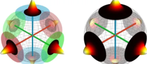
Fig. 1: Illustrations of the two probabilistic Manhattan Frame representations utilized by the proposed Real-time Manhattan Frame (RTMF) inference algorithms. Left: the tangent-space Gaussian model. Right: the von-Mises-Fisher-based model.
Inference of MW properties of the environment has been addressed previously by extracting and tracking vanishing points (VP) from camera images [1], [4], [7]. This approach utilizes the connection between VPs and 3D MW structure via projective geometry [8]: lines defined by intersections of surfaces of the MW projected into the camera intersect in VPs. Hence the location of VPs in the image depends on the rotation of the camera with respect to the surrounding MW. Following the approach of [3], we focus on surface normal data, such as can be extracted from representations of 3D structure including depth images or point clouds. Surface normals can be treated as observations of the orientation of the planes that constitute the surrounding local MW. We adopt their concept of a Manhattan Frame (MF) to describe the distribution of surface normals generated by a MW. See Fig. 1 for an illustration. In contrast to VP-based methods, which utilizes sparse observations of lines in the camera image, the proposed surface-normal-based approach takes advantage of the availability of dense observations due to planar structures in the scene.
Our contributions are threefold: first, we derive an ap-proximation to the tangent-space model of [3] which enables real-time maximum a posteriori (MAP) inference of the local MF. Second, we propose a novel MF model, depicted in Fig. 1, which utilizes the isotropic and circular von-Mises-Fisher (vMF) [9] distribution and lends itself to even more efficient inference. Third, we detail a GPU-supported real-time MF inference (RTMF) implementation which enables accurate Rotation tracking of dynamic and full 3D camera motion in typical indoor environments. We show how to further improve the resulting rotation estimates by fusing them with IMU rotational velocities in a standard EKF. In addition to the MW rotation estimate, the RTMF algorithm also provides a segmentation of the RGB-D frame into the six directions of a MW, which may be used for further processing.
II. RELATEDWORK
The use of the MW assumption for tracking the rotation of a camera and using surface normals for estimating MW rotations have both been considered previously. While the initial work on MW rotation estimation [1] framed VP estimation as a Bayesian inference problem on the full RGB image, the multi-stage approach [7] of first extracting line segments and then estimating VPs as the intersection-points of those segments has become popular [4], [10], [11]. VP-based MW rotation estimation from an RGB camera was used to estimate orientations within man-made environments for the visually impaired by Coughlan et al. [1] and for robots by Bosse et al. [4] where incorporation of MW orientation estimates resulted in significant reduction in drift. Flint et al. [12] integrate information across a stream of RGB images to obtain a semantic segmentation of the scene which relies on the MW structure of the observed environment.
Several approaches utilize depth or surface normal ob-servations to improve VP-based MW orientation estimation. Neverova et al. [10] integrate VP extraction from the RGB image with entropy minimization of the projection of the point cloud onto the MW directions for MW orientation estimation. Silberman et al. [11] rank VP-based [7] MW orientation proposals according to their alignment with sur-face normals extracted from the depth image. Purely sursur-face- surface-normal-aided MW estimation has been explored previously by Furukawa et al. [13] who employ a greedy algorithm for a single-MF extraction from normal estimates that works on a discretized sphere.
Besides VP-based MW rotation estimation by Bosse et al., Peasley et al. [5] demonstrate the use of a MW constraint directly within a pose-graph based SLAM setup. The 2D orientation of a robot with respect to the surrounding MW is estimated by extracting the dominant direction in a hor-izontal scan-line of the depth image using RANSAC. The resulting drift reduction allows direct integration of RGB-D measurements into an octree representation of the world. In contrast to the proposed method, [5] relies on the assumption that the camera is constrained to movements in a 2D plane.
III. MANHATTANFRAME(MF)
The use of aManhattan Frame(MF) [3] facilitates incor-porating the geometric and manifold properties of rotations into a probabilistic model suitable for inference. Here, this manifests as inference of rotation matrices from surface nor-mal observations. MFs are defined as the set of all planes that are parallel to one of the three major planes of an orthogonal coordinate system. Hence, they can be represented by a rotation matrixR∈SO(3). In practice, planes are observed indirectly via noisy surface-normal measurements extracted, e.g., from depth images or LiDAR data. As such, it is useful to think of a MF as the set of normals that are aligned with one of the six orthogonal directions{µk}6k=1 parameterized
byR and−R:
[R,−R] = [µ1, . . . , µ6] ⇔ µk= sign(k)Rkmod3, (1)
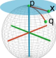
Fig. 2: The axes of an MF displayed in RGB within the unit sphereS2. The blue plane showsT
pS2, the tangent space to
S2 at pointp. A vectorx∈T
pS2 is mapped toq∈S2 via
Expp, the Riemannian exponential map with respect top.
wheresign(k)is1fork <3and−1fork≥3andRkmod3
selects the(kmod3)th column ofR. A. The Manifold of the Unit SphereS2
The unit sphere S2 is a two-dimensional Riemannian
manifold whose geometry is well understood. As such, we represent surface-normals as points onS2. We make use of
the following properties, intrinsic to the unit sphere S2 in
3D, for reasoning over the rotation of a MF [14], [15]. Let pand q be two points inS2. The geodesic distance betweenpandq is given by [14]
dG(p, q) = arccos(pTq). (2)
That is, the geodesic distance (i.e., the distance along the manifold) between two unit normals is equal to the angle between them.
A second important concept is the notion of a tangent space to the sphere at a point p denoted TpS2. Figure 2
illustrates this concept. We can use the Riemannian Expo-nential map Expp(x) to map a point x∈ TpS2 back onto
the sphere and the inverse, the Riemannian Logarithm map Logp(q), to map a pointq∈S2into the tangent spaceT
pS2.
Mathematically, these maps are computed as: Expp(x) =pcos(||x||2) + x ||x||2 sin(||x||2) (3) Logp(q) = (q−pcosθ) θ sinθ, (4) whereθ=dG(p, q) =||x||2.
The Karcher mean qe of a set of points on a manifold {qi}Ni=1is a generalization of the sample mean in Euclidean
space [16]. It is a local minimizer of the following weighted cost function: e q= arg minp∈MXN i=1wid 2(p, q i). (5)
Here,wi = 1,M =S2, and d(·,·) =dG(·,·) In this case,
excepting degenerate sets, it has a single minimum. It may be computed by the following iterative algorithm:
1) project all{qi}Ni=1 intoTqetS
2and compute their
sam-ple meanx¯= N1 PN i=1Logqet (qi). 2) project x¯ from T e qtS
2 back onto the sphere to obtain e
qt+1= Exp
e
qt(¯x).
IV. MANHATTANFRAMEESTIMATION USING THE
TANGENTSPACE MODEL
As proposed in [3], a generative model for the MF using Riemannian geometry describes a surface normal, qi, as
generated from a zero-mean Gaussian distribution in the tangent space around its respective associated MF axisµzi.
R∼Unif(SO(3)) zi ∼Cat(π)
qi∼ N(Logµzi(qi); 0,Σ)
(6) The joint distribution of this model is:
p(z,q, R;π,Σ) =p(R)
N
Y
i=1
πziN(Logµzi(qi); 0,Σ). (7)
In the absence of further knowledge about the scene, the surface normals are assumed to be generated with equal probability from any of the axes, i.e. allπk= 16. For the same
reason we assume the same small and isotropic covariance Σ =σ2I for all MF axes.
Starting from this probabilistic MF model we first derive the MAP inference directly before introducing an approxi-mation to improve efficiency.
A. Direct MAP MF Rotation Estimation
Starting from the joint distribution of the tangent space MF model in Eq. (7), we derive the direct MAP MF rotation estimation. The posterior over assignments zi of surface
normalsqi to axis of the MF is given by
p(zi=k|R, qi;π,Σ)∝πkN(Logµk(qi); 0,Σ). (8) Therefore the MAP estimate for the label assignment zi
becomes: zi = arg min k∈{1...6} Logµ k(qi) TΣ−1Log µk(qi) = arg min k∈{1...6} arccos2(qiTµk), (9)
where we have usedarccos(qT
i µk) =||Logµk(qi)||2 and the assumption that the covarianceΣis isotropic.
With p(R) = Unif(SO(3)), the posterior over the MF rotation Ris p(R|q,z; Σ)∝p(q|z, R; Σ)p(R)∝p(q|z, R; Σ) = = N Y i=1 N(Logµzi(qi); 0,Σ). (10)
Working in the log-domain, the MAP estimate forR is:
R?= arg min
R
−logp(R|q,z; Σ) := arg min
R
f(R). (11) Plugging in the posterior from Eq. (10) we obtain:
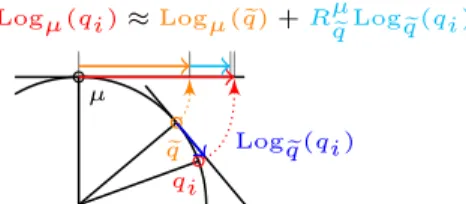
f(R) =−log "N Y i=1 N(Logµ zi(qi); 0,Σ) # ∝ N X i=1 Logµ zi(qi) TΣ−1Log µzi(qi) ∝ N X i=1 arccos2(qiTµzi), (12) µ e q qi Log e q(qi) Logµ(qi)≈Logµ(q)e +R µ e qLogqe (qi)
Fig. 3: Illustration of the geometry underlying the approxi-mation of the mapping ofqi intoTµS2 viaLogµ(qi).
where we have used the same trick as in Eq. (9). This method is called direct since the cost function directly penalizes the deviation of a normal from its assigned MF axis.
We enforce the constraints onRby explicitly optimizing the cost function on theSO(3)manifold. Specifically, we em-ploy the conjugate gradient optimization algorithm from [17], which is also summarized in Alg. 1. Note, that the SO(3) manifold is equivalent to a3×3 Stiefel manifold.
With i = arccos(qiTµzi) and Ik = {i | zi = k}, the JacobianJ = [J0, J1, J2]∈R3×3 for the optimization is:
Jk = ∂f(R) ∂Rk = X i∈Ik∪Ik+3 2 sign(zi)i p 1−(qT i µzi) 2qi. (13)
B. Approximate MAP MF Rotation Estimation
The direct approach derived in the previous section is inefficient since the cost function in Eq. (12), as well as the respective Jacobian, involves a sum over all data-points. These quantities need to be re-computed after each update toR in the optimization. Especially the required line-search along theSO(3)manifold required by the conjugate gradient optimization algorithm (c.f. line 8 of Alg. 1) makes the direct approach computationally expensive since it requires a significant number of cost function evaluations per iteration. To address this inefficiency, we derive an approximate estimation algorithm by exploiting the geometry of the manifold of the unit sphere.
The approximation necessitates the computation of the Karcher means {qek}6k=1 for each of the sets of normals
associated with the respective MF axis. After this preparation step, we approximateLogµ(qi)using the Karcher meanqezi of its associated set of data{qi}Izi:
Logµ(qi)≈Logµ(eq) +R µ e qLogeq(qi). (14) where Rµ e q rotates vectors in TqeS 2 to T µS2 as proposed
in [18]. Intuitively this approximates the mapping ofqi into
µzi by the mapping of the Karcher mean into µzi plus a correction term that accounts for the deviation ofqifrom the
e
qzi. See Fig. 3 for an illustration of underlying geometry. With this the cost function f(R) from Eq. (12) can be
Fig. 4: 2D vMF distributions with concentrationsτ= 1(left) andτ= 100 (right) around meanµ= (p1/2,p1/2).
approximated by f˜(R)as: f(R)≈f˜(R)∝ N X i=1 Logµ zi(qi) TΣ−1Log µzi(qi) ∝ 6 X k=1 X i∈Ik Logµ k(qek) TLog µk(qek) + 2Log e qk(qi) T(Rµk e qk) TLog µk(qek) = 6 X k=1 |Ik|arccos2(qe T kµk), (15)
where we have used that the sample mean in the tangent space of the associated Karcher meanP
i∈IkLogeqk
(qi)T =
0 by definition. The Jacobian for this approximate cost function thus becomes:
Jj = ∂f˜(R) ∂Rj = X k∈{j,j+3} 2 sign(k)|Ik|k q 1−(qeT kµk)2 e qk, (16)
where k = arccos(qeTkµk). Thus the optimization of the
MF’s rotation only utilizes the Karcher means {qek}6k=1,
which can be pre-computed. The need to iterate over all data-points inside the optimization is eliminated.
V. MANHATTANFRAMEESTIMATION USING VON-MISES-FISHER DISTRIBUTIONS
In this section, instead of assuming tangent-space Gaus-sian distributions, we explore modeling the surface normals as von-Mises-Fisher (vMF) [9], [19] distributed. This distri-bution is natively defined over the manifold of the sphere and commonly used to model directional data [20], [21], [22], [23]. We show that the structure of the vMF distribution lends itself to even more efficient MAP inference.
A. Probabilistic MF-vMF model
The von-Mises-Fisher distribution defines an isotropic distribution for data {qi}Ni=1 on the sphere around a mean
directionµ with a concentrationτ and has the form: vMF(q;µ, τ) =Z(τ) exp(τ qTi µ) (17) whereZ(τ)is the normalizing constant. See Fig. 4 for a 2D illustrative example. Similar to the previous model, the MF can be described as a mixture model where we use vMF distributions as the observation model for the normals qi.
Again, lacking prior knowledge of the scene, we assume that
the normals are uniformly generated from the six axes, i.e.
πk =16, and that the vMFs have the same concentrationτ:
R∼Unif(SO(3)) zi∼Cat(π)
qi ∼vMF(qi;µzi, τ).
(18) The joint distribution for this model thus is:
p(z,q, R;π, τ) =p(R)
N
Y
i=1
πzivMF(qi;µzi, τ). (19)
B. MAP Inference in the MF-vMF Model
For the vMF-based MF model we derive the MAP estimate first for the labelszand then the MF’s rotationR. With the uniform distribution over labels, i.e. πk = 16, the posterior
distribution over labelzi follows the proportionality:
p(zi=k|qi, R;τ)∝vMF(qi;µk, τ)∝exp(τ qiTµk). (20)
Since we assume equal concentration parameterτfor the six vMF distributions, the MAP assignment forzi is:
zi= arg max k∈{1,...,6}
qTi µk. (21)
The MAP estimate for the MF rotation is derived using the posterior distribution:
p(R|q,z;τ)∝p(q|z, R;τ)p(R)∝p(q|z, R;τ) = = N Y i=1 vMF(qi|µzi;τ). (22)
Similar to the previous section the cost function fvMF(R)
which is minimized by the optimalR? is:
fvMF(R) =−logp(R|q,z;τ)∝ − N X i=1 τ qTi µzi ∝ − 6 X k=1 X i∈Ik qi !T µk. (23)
The final expression is rearranged to reveal the efficiency of this cost function: at each time-step the sums over data-points belonging to each MF axis can be pre-computed.
The Jacobian can also be expressed in terms of these sums:
Jj= ∂fvMF(R) ∂Rj = X k∈{j,j+3} −sign(k)X i∈Ik qi. (24)
VI. REAL-TIMEMANHATTANFRAMEINFERENCE
To achieve real-time operation of the three different kinds of MF inference algorithms on the full 640×480 depth image, we exploit parallelism in computing normals from the depth image, normal assignments to MF axes, as well as cost function evaluation. Additionally, we show that most of the data can remain in GPU memory. Only small matrices need to be copied out to the CPU. This is important, because moving data between CPU and GPU is time-intensive.
To reduce the number of conjugate gradient iterations, the MF rotation estimation at each frame is initialized from the previous frame’s rotation. This also eliminates the need to
Algorithm 1Optimization over the MF rotationR∈SO(3). The difference between the proposed approaches (direct, approximate and vMF-based) is in how the labels {zi}Ni=1
and the Jacobians are computed and which statistics are used.
1: InitializeR0(to the previous timestep’s frame rotation) 2: On GPU: Obtain {zi}Ni=1 using Eq. (9) or (21) 3: On GPU: compute statistics (approx. and vMF-based)
4: ComputeJ0 using Eq. (13), (16) or (24) respectively 5: G0=J0−R0J0TR0
6: H0=−G0
7: fort∈ {1. . . T} do
8: Rt= arg minR∈SO(3)along directionHt−1f(R)
9: ComputeJtusing Eq. (13), (16) or (24) respectively
10: Gt=Jt−RtJtTRt 11: if t mod 3 = 0then 12: Ht=−Gt 13: else 14: Ht=−Gt+tr{(Gtrt−{GGt−1)Gt} tGt} Ht−1Mmin 15: end if 16: end for 17: return RT
reason about the inherent90◦ ambiguity of the MF rotation estimate from frame to frame even for fast dynamic motions (see Sec. VII-D). Intuitively, as long as the rotation of the camera between two frames is less than45◦ about any axis of rotation, the MF rotation estimate will consistently track the same MF orientation without slipping to one of the other equivalent MF rotations describing the same MW.
A. Smooth Surface Normal Extraction from Depth Images We extract surface-normals from the depth image by performing, per point, a cross product of local gradients of the point cloud in image column and row direction. This approach hinges on a “clean” depth image since the local gradients are sensitive to noise.
We pre-process the depth image with an edge-preserving filter which accounts for depth discontinuities. These are ubiquitous in indoor environments. Iterative approaches such as anisotropic diffusion [24], [25] which simulates a dif-ferential equation to obtain increasingly smoothed images while preserving edges are not suitable for real-time op-eration. Among the fastest edge-preserving filters are the bilateral [26] as well as the guided filter [27]. We found the guided filter to yield the fastest edge-preserving algorithm in practice. In contrast to the bilateral filter, its time complexity is independent of the kernel size since integral images can be utilized. Additionally fast implementations of the bilateral filter usually rely on approximations [28].
After applying the guided filter we compute the point cloud from the smoothed depth image. For each, the x, y, andz, channel of the point cloud, a convolution with Sobel kernels yields approximate gradients pu = [xu, yu, zu] and
pv= [xv, yv, zv]in the image coordinate system. Finally, we
can compute surface-normals for each 3D point as the vector
orthogonal to these two local gradients:
q= pu×pv |pu×pv|
. (25)
Note that this operation is equivalent to the Gauss map [29] for regular surfaces.
All operations, convolutions as well as the cross products, are implemented on the GPU. The only necessary significant memory copy is moving the depth image into the GPU mem-ory. The MF rotation-estimation never needs the normals in CPU memory, but performs all operations involving normals entirely on the GPU. Depending on the inference algorithm statistics of the data, Jacobians and cost-function values are computed on the GPU and copied to CPU memory. B. Fusion of MF Rotations with Rotational Velocity Sensors
As alluded to in the introduction one important property of the MF rotation estimate is that it is a drift-free, absolute measurement with respect to the surrounding structure of the environment. Therefore, it can be used as an external refer-ence to correct the bias of orientation tracking systems that rely on integrating rotational velocities such as gyroscope or wheel-odometry sensors. If the bias is not corrected it is integrated together with the rotational velocities and thus causes the rotation estimate to drift.
We utilize an EKF to fuse rotational velocity measure-ments with the inferred absolute RTMF rotations. As pro-posed in [30] the state of the EKF contains the estimated fused rotation represented as a Quaternion and the bias of the sensor. While the rotational velocities measurements are used for the EKF prediction step, the RTMF rotation estimate is used in the update step. The observation model is straight forward since we directly observe the rotation via the RTMF algorithm. The uncertainty of the rotation estimate is set to a fixed value. Derivation of a method for estimating the uncertainty in the MF rotation is left for future research.
VII. RESULTS
We give qualitative and quantitative comparison of all three derived algorithms on several datasets. First, we evalu-ate the run-times and the rotation estimation accuracy of the different algorithms on a dataset with groundtruth data from a Vicon motion capture system. Second, we show rotation estimates for a large-scale indoor environment around Killian Court of MIT. Third, we show the MW segmentation of a set of scenes from the NYU depth dataset [11]. All evaluation was run on an Intel Core i7-3940XM CPU at 3.00GHz with a NVIDIA Quadro K2000M GPU.
With the goal of achieving real-time MF estimation, we use the following parameters throughout the whole evalua-tion. The direct RTMF algorithm was run for at most ten conjugate gradient iterations per frame with ten line-search steps each. Any fewer iterations rendered the MF rotation estimation unusable. For the approximate and the vMF-based RTMF algorithm we exploit the efficiency of the rotation optimization which uses only pre-computed statistics of the data. Hence we can run the conjugate gradient optimization for at most 25 iterations with 100 line-search steps each.
[de g] [%] de viation from V icon [de g]
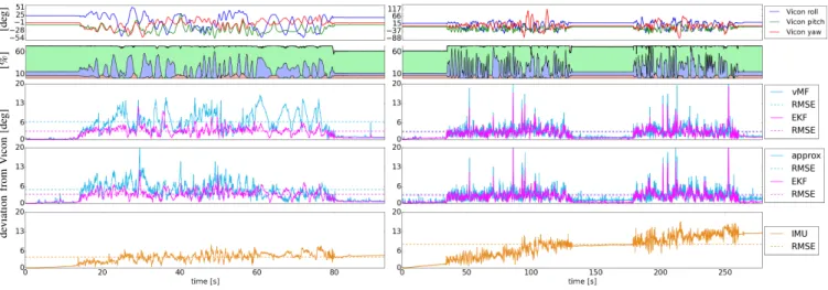
Fig. 5: Two different datasets with groundtruth data (first row). The percentages of points associated to a respective MF axis over time is color-coded in the second row. Rows two to four show the angular deviation from the groundtruth of the approximate as well as the vMF-based RTMF algorithm with and without fusion with the IMU. The IMU orientation estimate is displayed in the last row. Note that the RTMF algorithms are drift free in comparison to the IMU.
Fig. 6: Timing breakdown for the three different MF infer-ence algorithms. The error bars show the one-σrange.
A. Estimation Accuracy and Timing on Groundtruth Data We obtained groundtruth data using a Vicon motion cap-ture system to track the full 3D pose of an Xtion RGB-D sensor with attached IMU. We use Horn’s closed form absolute orientation estimation approach [31] to calibrate the IMU-Vicon-camera system. The datasets for this evaluation were obtained by waving the camera randomly in full 3D motion up-down as well as left-right in front of a wall with a rectangular pillar. The yaw, pitch, and roll angles of the Vicon groundtruth are displayed in the first row of Fig. 5.
1) Accuracy: Besides the evaluation of the rotation esti-mates of the proposed RTMF algorithms, we show the ro-tation estimates obtained by integrating roro-tational velocities measured by a Microstrain 3DM-GX3 IMU using an EKF as described in Sec. VI-B. Since the direct method is not real-time capable, we omit accuracy evaluation for it.
For the shorter groundtruth dataset of 90 s length, dis-played to the left in Fig. 5, we obtain an angular RMSE of the vMF-based MF rotation estimate from the Vicon groundtruth rotation of6.36◦and4.92◦for the approximate method. The IMU rotation estimate drifts and exhibits an RMSE of3.91◦. Note that while the drift can be reduced by incorporating IMU acceleration and magnetic field data, it can not be fully eliminated. Fusing the RTMF rotation estimates with the IMU using the EKF achieves even lower RMSEs of 3.05◦ for the vMF-based and3.28◦ for the approximate method.
Figure 5 to the right shows the angular deviation from Vi-con groundtruth during a longer sequence of about 4:30 min taken at the same location. Similar to the shorter sequence, the two MF rotation estimation algorithms exhibit zero drift and an RMSE below 3.4◦. The drift of the IMU is clearly observable and explains the high RMSE of8.50◦. The fusion of the rotation estimates using the Quaternion EKF again improves the RMSEs to below2.8◦.
The percentages of surface normals associated with the MF axes displayed in the second row of Fig. 5 support the intuition that a less uniform distribution of normals across the MF axes results in a worse rotation estimate: large angular deviations occur when there are surface normals on only one or two MF axes for several frames.
The lower RMSE of the EKF rotation estimates results from improving the estimate using the gyroscope when the MF estimation is not well constrained due to skewed distributions of surface normals across the MF axes. This highlights the complementary nature of the fusion approach: the IMU helps support rotation estimates on short timescales when the MF inference problem is not well constrained. In turn the RTMF rotation estimates help estimate and thus eliminate the bias from the gyroscope measurements.
2) Timings: We divide up the computation times into the following stages of the proposed algorithms: (1) applying the guided filter to the raw depth image, (2) computing surface normals from the smoothed depth image, (3) pre-computing of statistics of the data and (4) conjugate gradient optimization for the MF rotation.
The timings shown in Fig. 6 were computed over all frames of the shorter90s dataset. The direct method cannot be run in real-time as it takes an average of105ms per frame. While the approximate method improves significantly over the direct algorithm it is still 12 ms slower than the vMF-based approach which runs in19.8ms per frame on average. Therefore both the approximate and the vMF-based RTMF
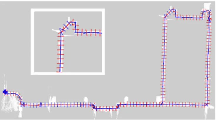
Fig. 7: MF orientations extracted as a Turtlebot V2 traverses the hallways around Killian court in the main building of MIT. The zoomed in area displays the top left corner of the loop. Note that the orientations align with the local MW structure of the environment.
algorithm can be run at a camera frame-rate of 30 Hz. The approximate and the vMF-based algorithm spend most of their time preprocessing the surface normal-data: while the approximate algorithm needs to compute the Karcher means for the six directions, the vMF-based approach needs to compute the sum over data-points for each direction. Using those statistics of the data, the conjugate gradient algorithm runs in a fraction of the time of the direct method, while allowing for more optimization iterations as well as a fine-grained line-search. In comparison to the vMF-based method the approximate algorithm is slower since the Karcher mean computation is an iterative procedure that computes on all data as described in Sec. III-A. In the following we omit the direct method from the evaluation due to its slow runtime. B. MF Inference for the large-scale Killian Court Dataset For this experiment a Turtlebot V2 robot equipped with a laser-scanner-based SLAM system was driven through the hallways surrounding Killian court in the main building of MIT. We ran the vMF-based RTMF algorithm on the depth stream from the Kinect camera of the robot. Figure 7 shows the inferred MF rotations every 200th frame at the respective position obtained via the SLAM system. It can be seen that the algorithm correctly tracks the orientation of the local MW. A part of the hallway on the top right does not align with the overall MW orientation and the estimated orientations are thus aligned with this local MW which is at an angle with respect to the rest of the map. This highlights that the MW assumption is best treated as a local property of the environment as argued in the introduction. In parts of the map without nearby structure the MW rotation estimate is off due to the lack of data.
C. Manhattan World Scene Segmentation
As a by-product of the MF rotation estimate the algorithm also provides a segmentation of the frame into the six different orthogonal and opposite directions. This segmen-tation can be used as an additional source of information for further processing. For example, using the direction of
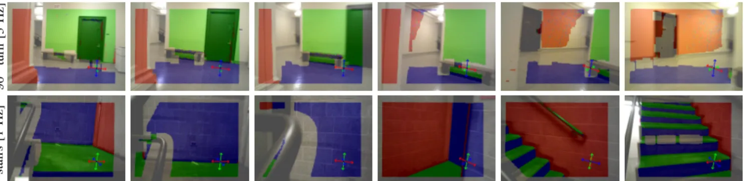
gravity it would be easy to extract the ground plane for obstacle avoidance. We show several examples of segmented scenes taken from the NYU depth dataset [11] in Fig. 8. The RTMF algorithms used the same parameters as before. The segmentations show that the vMF-based and the approximate method perform well on a wide range of cluttered scenes. The direct algorithm with a fine-grained line-search in the conjugate gradient optimization give similar results to the two other approaches but is significantly slower.
D. Manhattan Frame Inference under dynamic Motion The proposed MF inference algorithm performs well even under highly dynamic motions such as running down a corridor with 90◦ turns or up a stair case. In Fig. 9 we show key frames from longer sequences which may be found in the supplementary video. While running around the 90◦ turn, the MF rotation is consistently tracked at rotational velocities of50◦s−1 and jerky motion. The video contains
several more examples of consistent tracking through rapid camera movement.
VIII. CONCLUSION
We have derived three MF rotation inference algorithms and demonstrated their usefulness and accuracy as a “struc-ture compass” providing absolute rotation estimates in envi-ronments with local MW structure in real-time. The rotation inference was surprisingly robust to fast and dynamic camera motions such as occur while running. Of the three, our evaluation demonstrates that the vMF-based algorithm runs both faster (∼20 ms per estimated MF) and with more reliable running time (i.e., low run time standard deviation) while delivering the same quality of rotation estimates as the other two approaches. Despite its longer run time, the direct method is useful for comparison purposes and poten-tially provides a more expressive representation as it allows for anisotropic scattering of normals about their respective means (though, we did not exploit this property in this presentation). While we have shown promising MW scene segmentations, we envision a host of potential applications, for example, in aiding semantic scene understanding where it is important to align the scenes to a common orientation before further processing [11], [32].
Future work will aim to obtain the global mixture of MW structure of the environment from the locally tracked MFs. Another avenue of research is integrating the MF labels into a 3D reconstruction pipeline for Manhattan Worlds.
All code and the supplementary video is available at
http://people.csail.mit.edu/jstraub/. REFERENCES
[1] J. M. Coughlan and A. L. Yuille, “Manhattan world: Compass direction from a single image by Bayesian inference,” in ICCV, 1999.
[2] G. Schindler and F. Dellaert, “Atlanta world: An expectation maximization framework for simultaneous low-level edge grouping and camera calibration in complex man-made environments,” in
CVPR, 2004.
[3] J. Straub, G. Rosman, O. Freifeld, J. J. Leonard, and J. W. Fisher III, “A mixture of Manhattan frames: Beyond the Manhattan world,” in
vMF
approx.
direct
-HQ
Fig. 8: In each row the MF segmentations of several scenes from the NYU depth dataset [11] are displayed for one of the different RTMF algorithms. The segmentation is overlaid on top of the grayscale image of the respective scene. The inferred MF orientation is shown in the bottom right corner of each frame. Unlabeled areas are due to lack of depth data.
90 ◦ turn [3 Hz] stairs [1 Hz]
Fig. 9: Extracted MFs when running around a90◦corner and briskly walking up stairs. Frame rates are indicated to the left.
[4] M. Bosse, R. Rikoski, J. Leonard, and S. Teller, “Vanishing points and three-dimensional lines from omni-directional video,”The Visual Computer, 2003.
[5] B. Peasley, S. Birchfield, A. Cunningham, and F. Dellaert, “Accurate on-line 3D occupancy grids using Manhattan world constraints,” in
IROS, 2012.
[6] O. Saurer, F. Fraundorfer, and M. Pollefeys, “Homography based visual odometry with known vertical direction and weak Manhattan world assumption,”ViCoMoR, 2012.
[7] J. Koˇseck´a and W. Zhang, “Video compass,” inECCV, 2002. [8] R. Hartley and A. Zisserman,Multiple View Geometry in Computer
Vision, 2004.
[9] N. I. Fisher,Statistical Analysis of Circular Data, 1995.
[10] N. Neverova, D. Muselet, and A. Tr´emeau, “2 1/2D scene reconstruction of indoor scenes from single RGB-D images,” in
Computational Color Imaging, 2013.
[11] P. K. Nathan Silberman, Derek Hoiem and R. Fergus, “Indoor segmen-tation and support inference from RGBD images,” inECCV, 2012. [12] A. Flint, D. Murray, and I. Reid, “Manhattan scene understanding
using monocular, stereo, and 3D features,” inICCV, 2011.
[13] Y. Furukawa, B. Curless, S. M. Seitz, and R. Szeliski, “Reconstructing building interiors from images,” inICCV, 2009.
[14] P. Absil, R. Mahony, and R. Sepulchre,Optimization algorithms on matrix manifolds. Princeton University Press, 2009.
[15] M. P. do Carmo,Riemannian Geometry. Birkh¨auser Verlag, 1992. [16] X. Pennec, “Probabilities and statistics on Riemannian manifolds:
Basic tools for geometric measurements,” inNSIP, 1999.
[17] A. Edelman, T. A. Arias, and S. T. Smith, “The geometry of algorithms with orthogonality constraints,” SIAM Journal on Matrix Analysis and Applications, 1998.
[18] J. Straub, J. Chang, O. Freifeld, and J. W. Fisher III, “A Dirichlet process mixture model for spherical data,” inAISTATS, 2015. [19] K. V. Mardia and P. E. Jupp,Directional statistics. John Wiley &
Sons, 2009.
[20] A. Banerjee, I. S. Dhillon, J. Ghosh, S. Sra, and G. Ridgeway, “Clustering on the unit hypersphere using von Mises-Fisher distributions.”JMLR, 2005.
[21] M. Bangert, P. Hennig, and U. Oelfke, “Using an infinite von Mises-Fisher mixture model to cluster treatment beam directions in external radiation therapy,” inICMLA, 2010.
[22] S. Gopal and Y. Yang, “von Mises-Fisher clustering models,” inICML, 2014.
[23] J. Straub, T. Campbell, J. P. How, and J. W. Fisher III, “Small-variance nonparametric clustering on the hypersphere,” inCVPR, 2015. [24] P. Perona and J. Malik, “Scale-space and edge detection using
anisotropic diffusion,”TPAMI, 1990.
[25] J. Weickert,Anisotropic diffusion in image processing. Teubner, 1998. [26] C. Tomasi and R. Manduchi, “Bilateral filtering for gray and color
images,” inICCV, 1998.
[27] K. He, J. Sun, and X. Tang, “Guided image filtering,” inECCV, 2010. [28] S. Paris and F. Durand, “A fast approximation of the bilateral filter
using a signal processing approach,” inECCV, 2006.
[29] M. P. do Carmo, Differential geometry of curves and surfaces. Prentice-hall Englewood Cliffs, 1976.
[30] N. Trawny and S. I. Roumeliotis, “Indirect Kalman filter for 3D attitude estimation,” University of Minnesota, Dept. of Comp. Sci. & Eng., Tech. Rep. 2005-002, 2005.
[31] B. K. Horn, “Closed-form solution of absolute orientation using unit quaternions,”JOSA A, 1987.
[32] S. Gupta, P. Arbelaez, and J. Malik, “Perceptual organization and recognition of indoor scenes from RGB-D images,” inCVPR, 2013.