Spiking Neural Networks for Inference and Learning: A Memristor-based Design Perspective

UC Irvine

UC Irvine Previously Published Works

Title

Spiking Neural Networks for Inference and Learning: A Memristor-based Design Perspective

Permalink

https://escholarship.org/uc/item/0bx5d5vv

Authors

Fouda, ME

Kurdahi, F

Eltawil, A

et al.

Publication Date

2019

License

https://creativecommons.org/licenses/by/4.0/ 4.0

Peer reviewed

Spiking Neural Networks for Inference and Learning: A

Memristor-based Design Perspective

M. E. Fouda, F. Kurdahi, A. Eltawil, E. Neftci

October 9, 2019

Abstract

On metrics of density and power efficiency, neuromorphic technologies have the potential to surpass mainstream computing technologies in tasks where real-time functionality, adaptability, and autonomy are essential. While algorithmic advances in neuromorphic computing are proceeding successfully, the potential of memristors to improve neuromorphic computing have not yet born fruit, primarily because they are often used as a drop-in replacement to conventional memory. However, interdisciplinary ap-proaches anchored in machine learning theory suggest that multifactor plasticity rules matching neural and synaptic dynamics to the device capabilities can take better advantage of memristor dynamics and its stochasticity. Furthermore, such plasticity rules generally show much higher performance than that of classical Spike Time Dependent Plasticity (STDP) rules. This chapter reviews the recent development in learning with spiking neural network models and their possible implementation with memristor-based hardware.

Keywords: Brain-inspired Computing, In-memory computing, Deep Learning, Memristors, Nonindeal-ities, Three-Factor Rules.

1

Introduction

Machine Learning and particularly deep learning have become thede facto choice in solving a wide range of problems when adequate data is available. So far, machine learning has been mainly concerned more by the “learning” rather than the “machine”. This focus is natural given that von Neumann computers and GPUs capable of general-purpose processing offer excellent performance per unit of monetary cost. As the scalability of such processors hit difficult scalability and energy efficiency challenges, interest in dedicated, multicore and multiprocessor systems is increasing. This calls for increased efforts on improving the physical instantiations of “machines” for machine learning. Physical instantiation of computations are challenging because the structure and nature of the physical substrate severely restrict the basic computational operations it can carry out. However, if the computations can be formulated in a way that they exploit the physics of the devices, then the efficiency and scalability can be drastically improved. In this line of thought, the field of neuromorphic engineering is arguably the one that has attracted the most attention and effort. The field’s core ideas, communicated by R. Feynmann, C. Mead and other researchers in a series of lectures called physics of computation, elaborate on the analogies between the physics of ionic channels in the brain and those of CMOS transistors [Mead, 1990]. By building synapses, neurons, and circuits modeled after the brain and driven by similar physical laws, neuromorphic engineers would “understand by building” and help engineering novel computing technologies equipped with the robustness and efficiency of the brain. In the last decade, there have been enormous advances in building and scaling neuromorphic hardware using mixed-signal [Benjamin et al., 2014, Chicca et al., 2013, Park et al., 2014, Schemmel et al., 2010] and digital [Merolla et al., 2014, Davies et al., 2018, Furber et al., 2014] technologies, including embedded learning capabilities and scales achieving 1M neurons per chip. A major limitation in these technologies is the memory required to store the state and the parameters of the system. For example, in both mixed-signal and digital technologies, synaptic weights are typically stored in SRAM, the densest, fastest and most energy-efficient memory we can currently locate next to the computing substrate [Qiao et al., 2015, Merolla et al., 2014, Davies et al., 2018]. Unfortunately, SRAMs are expensive in terms of area and energy, making on-chip memory small given

the computational requirements. In fact, learning often requires higher precision parameters to average out noise and ambiguities in real-world data, especially in the case of gradient-based learning in neural networks [Courbariaux et al., 2014].

With this premise, in this chapter, we explore promising learning and inference algorithms compatible with neuromorphic hardware, with a special focus on spiking neural networks. We highlight their hard-ware requirements, discuss their possible implementations with memristors and finally, identify a class of computations they are particularly suitable for. In so doing, we will view spiking neural networks as types of recurrent neural networks and explain which hardware non-idealities are detrimental, and which can be exploited for improving computations.

2

Models of Spiking Neural Networks and Synaptic Plasticity

We start with a description of neuron models commonly used in neuromorphic hardware and then describe the tools used to analyze and develop algorithms on them. The most common model is the Leaky Integrate & Fire (LI&F) [Indiveri et al., 2011]. While several variations of LI&F neuron models of it exist, including mixed-signal current-mode and digital implementations, the base model can be formally described in differential form as: τmem dUi dt =−(Ui−Urest) +RIi−Si(t)(Ui−Urest), (1) τsyn dIi dt =−Ii(t) +τsyn X j WijSj(t), (2)

where Ui(t) is the membrane potential of neuron i, Urest is the resting potential, τmem and τsyn are the

membrane time constants, R is the input resistance, and Ii(t) is the synaptic current [Gerstner et al.,

2014]. Eq. (1) shows that Ui acts as a leaky integrator of the input current Ii, which itself is a leaky,

weighted integration of the spike train Sj. Spike trains are described as a sum of delta Dirac functions

Sj(t) =P_kδ(t−tkj)tkj where tkj are spike times of neuronj. In other words, for each incoming spike, the

synaptic current undergoes a jump of heightWij and otherwise decays exponentially with a time constant

τsyn. Note that the expression P_jWijSj(t)has the structure of a vector-matrix multiplication, and forms

the basis of RRAM implementations of Spiking Neural Networks (SNNs) discussed later in this chapter. BecauseSj represents spikes (Sj = 0or1), these operations consist in additions and scaling of the result by

τsyn.

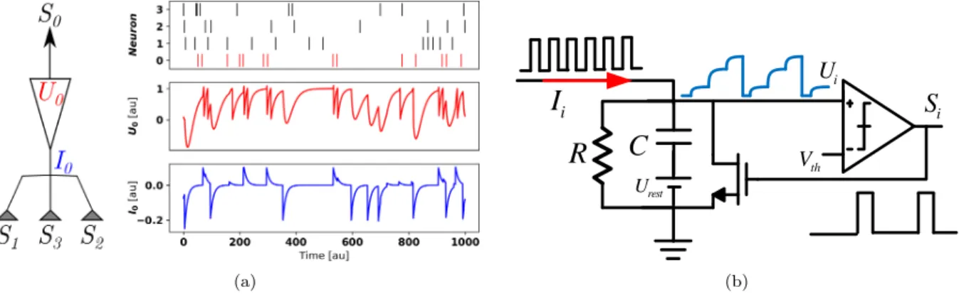
Neurons emit spikes when the membrane voltage reaches the firing threshold, Vth. After each spike, the

membrane voltageUiis reset to the resting potentialUrest(Fig. 1a). In Eq. (1), the reset is carried out by the

termSi(t)(Ui−Urest)when the membrane potential reachesVth. This reset acts as a refractory mechanism

since the neuron must reach the firing threshold fromUrest to fire again.

A simple circuit implementation of the LI&F is based on resistor-capacitor circuits with a switch to reset the voltage across the capacitor as shown in Fig. 1b. The mathematical model of this circuit is equivalent to Eq. (1) where τmem = RC. Several variations of this circuit have been demonstrated [Indiveri et al.,

2011]. Synaptic circuits which reproduce the dynamics of I can be implemented in analog VLSI using a Differential-Pair Integrator (DPI) or other similar circuits [Bartolozzi and Indiveri, 2007].

To make the mathematical analysis and digital implementations more intuitive, it is useful to write LI&F in the discrete form:

Ui[n+ 1] =βUi[n] +Urest+Ii[n]−Si[n](Ui[n]−Urest)

Ii[n+ 1] =αIi[n] + X j WijSj[n] Si[n] = Θ(Ui[n]) = 1 Ui[n]≥Vth 0 Otherwise where α= exp(− ∆t τmem), β = exp(− ∆t

τsyn) are constants that capture the decay dynamics of statesU andI

(a) i

U

R

C

i

I

S

_i rest U th V (b)

Figure 1: a)Example Leaky Integrate & Fire Neuron dynamics forUrest= 0andVth= 1and b) basic neuron

circuit implementing LI&F dynamics.

Several digital implementations of spiking neural networks use these update equations [Detorakis et al., 2018b, Davies et al., 2018]. These equations are can be described using an artificial Recurrent Neural Network (RNN) [Neftci et al., 2019] formalism. The recurrent aspect arises from the statefulness of the neurons (whenα >0andβ >0). In addition, if there exist connections from the neuron to itself, then these connections can be viewed on the same footing as recurrent connections in artificial RNNs. As we shall later see, the artificial RNN view of spiking neural networks enables the derivation of biologically credible learning rules with the capabilities of machine learning algorithms.

This description of the spiking neural network generalizes to a non-recurrent artificial neural network where activations are binary. In fact, replacingαandβ with 0 and ignoring the reset, the equations above become: Ui[n+ 1] = X j WijSj[n], Si[n] = Θ(Ui[n]). (3)

The dynamics above are those of the standard artificial neural network (without any multiplications, as described above) followed by a spiking nonlinearity, i.e. they are Perceptrons. Neural networks with bi-nary neural activations and/or weights were proposed as efficient implementations of conventional neural networks [Courbariaux et al., 2016, Rastegari et al., 2016]. Such devices are promising for energy-efficient implementations of deep learning processors in full-digital technologies [Andri et al., 2016, Umuroglu et al., 2017] as well as with in-memory processing with emerging memory devices [Sun et al., 2018].

3

Memristive Realization and Non-idealities

Neuromorphic hardware implementations require a device or a circuit that mimics the synapse behavior. A minimum requirement for neural network applications is a memory to store the synaptic weight. Memristive devices can be used to realize these such synapses. A device is referred to as a memristive device if it exhibits pinched hysteresis behavior in the current-voltage plane which indicates a memory behavior in its resistance. Many physical devices exhibit memristive behaviors such as Phase Change Memory (PCM), ferroelectric RAM (FeRAM), spin-transfer torque magnetic RAM (STT-MRAM), and resistive RAM (RRAM or ReRAM). RRAMs have a promising potential for neuromorphic applications due to high area density, stackability, and low write energy, compared to the other emerging devices [Wilson, 2013]. Thus, in this section, we focus on RRAM, without loss of generality, to discuss the physical limitations and problems facing deploying such technology for neuromorphic hardware.

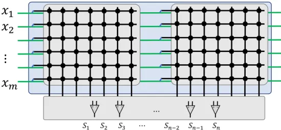
A common building block in both spiking and non-spiking neural network is the weighted summation of inputs (see Eq. (3)). This can be performed in a single step using a crossbar structure, unlike the conventional computing methods which typically requireN×M steps or clock cycles. Fig. 2 shows a single-layer crossbar based resistive neural network with M inputs and N outputs representing N perceptrons with M inputs each and the weights are stored in the memristors. The inputs to the perceptrons (presynaptic signals)

𝑥

₁

𝑥

₂

⋮

𝑥

_𝑚

𝑆1 𝑆2 𝑆3 ⋯ 𝑆𝑛−2 𝑆𝑛−1 𝑆𝑛 + − + − + − + − ⋯

Figure 2: Crossbar array realization of one layer neural network.

are encoded in the input voltages, and the output of each perceptron is the sum of the currents passing through each memristor. This way, all currents within the same column can be linearly summed to obtain the postsynaptic currents, i.e. the equivalent of Eq. (2). The total postsynaptic currents need sensing and shaping circuits to convert them into voltages and passed to subsequent neurons. In a nonspiking neural network, the postsynaptic current is summed up through the sensing circuit and passed through another shaping circuit to create the required neural activity such as sigmoid, tanh or rectified linear functions. With spiking neurons, the output of the current sensing circuit is instead passed through a LI&F circuit.

In neural networks, both positive (excitatory) and negative (inhibitory) connections are required. How-ever, the RRAM conductance is positive by definition which only supports excitatory or inhibitory connec-tions. Two weight realization techniques are possible to create both excitatory and inhibitory connections;

1) using two RRAMs per weight [Prezioso and et al., 2015, Li and et al., 2018] or

2) using one RRAM as weight in addition to one reference RRAM having a conductance set to Gr =

(Gmax+Gmin)/2 [Chang and et al., 2017, Fouda et al., 2018b].

The first realization has double the dynamic range w∈[−∆G,∆G], where∆G=Gmax−Gmin, making

it more immune to variability at a cost of double the area, double power consumption during reading and additional programming operations. The second technique has one RRAM device, meaning that w∈

[−∆G/2,∆G/2]making it more prone to variability but the overall area is smaller, requires less power, and is easier to program (programming only one RRAM per weight). Due to the high variations in the existing devices, the first approach is commonly used with either one big crossbar or two crossbars (one for positive weights and the other one for negative weights as shown in 2). The output of the memristive neural network can be written as Si = m X j=1 GijVj (4)

whereSiis the output of theithneuron andGij =G+ij−G

−

ij, is the synaptic weight, andVj is thejthinput.

The crossbar array forms the majority of the research in using RRAMs for neuromorphic computation [Yu, 2018]. In practice, RRAMs and crossbar structures suffer from many problems and do not behave ideally for computational purposes. These non-idealities can severely undermine the overall performance of applications unless they are taken into consideration while the training operation. After defining the mapping of synaptic weights to RRAM conductances, the following sections will overview these non-idealities in the light of neuromorphic computation and learning.

𝑊 ∝

𝐺

+

₋

_𝐺

−

𝐺

_𝑚𝑎𝑥

𝐺

_𝑚𝑖𝑛

−𝑊

_𝑚𝑎𝑥

𝑊

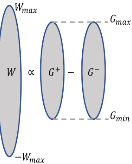
𝑚𝑎𝑥

Figure 3: Mapping synaptic weight into conductances.

3.1

Weight Mapping

As discussed above, each weight is translated into two conductances which is one-to-two mapping which can be mathematically formulated as

G=G+−G− = W Wmax

∆G, (5)

where Wmax is the maximum value of the weight. If it is required to realizeWmax, G+ andG− are set to

Gmax and Gmin, respectively. The difference between the two conductances is constant and proportional

to the required weight value and each conductance is constrained to be betweenGmin andGmax as shown

in Fig. 3. Thus, there are many possible realizations for each weight; for example, the zero weight can be realized with any equal values ofG+ _andG−_{. Therefore, a criterion for selecting the weight mapping should}

be defined. This can be formulated as an optimization problem as follows: minimize L(_G+,_G−)

subject to

Gmin≤G+, G− ≤Gmax,and

G+−G− =_WW

max

∆G.

(6)

where L is the objective function (objective function are discussed in further detail later in this chapter).

G+ and G− are the positive and negative conductance matrices. Since many conductance configurations

are possible to obtain the same effective weight, additional criteria such as power consumption while reading (important for inference) or the write energy (important in online training) can be introduced. These constraints can be taken into consideration while training the network with a regularization term in the loss function (see Sec. 4). We note that the mapping is more important for offline training where the optimization is completed on software and the final weight values are transferred to the hardware.

3.2

RRAM endurance and retention

An attractive purpose of RRAMs is to accelerate inference and training. However, endurance is a critical obstacle to RRAM deployment in neuromorphic hardware. In online learning, the devices are frequently updated, and especially so during gradient-based learning such as in artificial neural networks. However, each device has a limited number of potentiation and depression cycles [Zhao et al., 2018, Chen et al., 2011]. Endurance depends on the device’s switching and electrode materials. For example,HfOxdevices can achieve

endurance, it is necessary to complete the training before the devices degrade. The endurance requirement for learning is application-dependent. In standard deep learning, weight updates are usually performed every batch. Classification benchmarks such as MNIST handwritten digit recognition require writing around104

cycles. However, even gradient-based training of neural networks can easily scale to108_cycles.

Furthermore, because neuromorphic hardware can be multi-purpose (i.e. the same device and be used to perform many different tasks), where a complete training of the network is performed for every task. Consequently, the device endurance should be high enough to cover its lifetime use. There are some solutions to mitigate the endurance problem in machine learning scenarios:

• Full offline training: training is completed off the device and the final weights are transferred to the RRAM-based hardware. This requires an accurate model of the devices, the crossbar array and the sensing circuitry in the training procedure, and to verify the response of each part of the network to make sure that the response matches the simulated one [Jain et al., 2018].

• Semi-online training: A complete training cycle is performed offline, then the new weights are trans-ferred to the devices. Then, online retraining is carried out to reduce performance loss due to the existing impairments. Due to the smaller number of writing cycles, this solution would relax the en-durance requirements. In [Fouda et al., 2018b], it was noticed that the network was able to recover the original accuracy after10∼20% of the training epochs.

Once the online or the offline training is performed, the network can operate in the inference mode where only reading cycles are performed. In this case, the retention of the stored values becomes an important issue. As with endurance, RRAM retention is also dependent on the device materials and temperature. For example, the HfOx devices have around 104 seconds (2.78 hours) retention [Azzaz et al., 2016]. Although

this might be sufficient for certain single-use scenarios, such as biomedical applications, it is inadequate for IoT and autonomous control applications. There, retention values need to be more than106 _{seconds across}

different temperature values (since retention degrades with increasing the temperature).

Full online learning requires high endurance and moderate retention, but, semi-online requires moderate endurance and retention. Thus, while both endurance and retention are important for machine inference and learning tasks, the learning approach may require one more over the other.

3.3

Sneak Path Effect

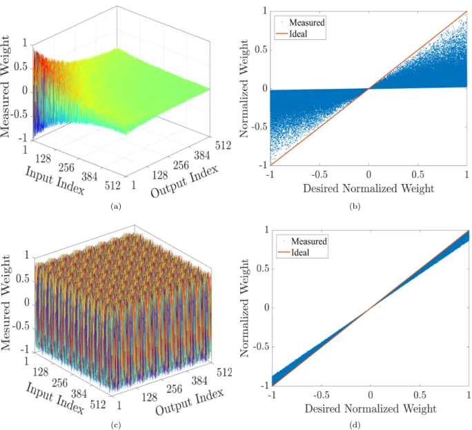
The sneak path problem, also is referred to as IR drop, arises from the existence of the wire resistance which is inevitable in nanostructure crossbar arrays. The wire resistance creates many paths to the signal from each the input port to the output port. These multiple paths create undesired currents which perturb the reading of the weight. It is expected that the wire residence would reach around92Ω for5nm feature size [Fouda et al., 2018a], which is the expected feature size for crossbar technology according to International Technology Roadmap of Semiconductors (ITRS) [Wilson, 2013]. Fig. 4a and Fig. 4b show an example of the sneak path problem in 512×512 with random weights. A linear switching device having a 106_{Ω high}

resistance state and103_{Ωlow resistance state is used while the wire resistance is0.1Ω. Ideally, the measured}

weights should be similar to the measured weights, as shown in Fig. 4c. Despite the small value of the wire resistance, it has a very high effect on the weights stored in the crossbar arrays (Fig. 4a). The weights are exponentially decaying across the diagonal of the array where the cell (1,1) has the least sneak path effect and the cell (N,M) has the worst sneak path effect.

Some devices have a voltage-dependent conductance where the conductance is an exponential or quadratic function of the applied voltage [Fouda et al., 2018a]. This conductance nonlinearity can help reduce the sneak path problem in resistive memories on crossbar or crosspoint structures [Fouda et al., 2019] due to single cell reading. But, in neuromorphic applications, this adds an exponential behavior to vector-matrix multiplication (VMM) which becomes

Si= m

X

j=1

Gijsinh(aVj). (7)

This exponential nonlinearity makes the VMM operation inaccurate which deteriorates the training per-formance [Kim et al., 2018]. Some algorithms were developed to take the effect of the device’s

voltage-(a) (b)

(c) (d)

Figure 4: Effect of the wire resistance on the measured weights for 512×512 crossbar array at with0.1Ω

wire resistance. 3D plots of random weights distributed across the array, (a) without partitioning and (c) with partitioning into64×64crossbar arrays; and the measured weights with the sneak path problem versus the desired values for (b) the entire array without partitioning and (d) with partitioning.

dependency into consideration while training non-spiking neural networks such as [Kim et al., 2018]. The same algorithm idea can be extended to spiking neural networks.

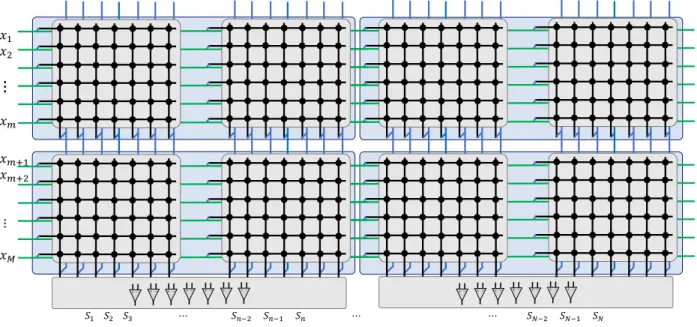
Partitioning of Large Layer Matrices The sneak path problem prohibits the implementation of large matrices using a single large crossbar array. One possible solution is to partition the large layer matrices into small matrices that can be implemented using realizable crossbar arrays. Figure 5 shows the partitioned crossbar arrays and the interconnect fabric between them to realize the complete VMMs where the large crossbar array, having N ×M RRAMs, is partitioned into n×m crossbar arrays. In order to have the same structure of a large crossbar array, vertical and horizontal interconnects are placed under the crossbar arrays. This horizontal interconnect is used to connect the inputs between the crossbar arrays within the same array rows. The vertical interconnect is used to connect the outputs of the vertical crossbar arrays. The vertical interconnects are grounded through the sensing circuit to absorb the currents within the same vertical wire. The sensed currents are connected then to the neuronal activity. It is worth highlighting that

each crossbar array may require input drivers (buffers) to reduce the loading effect of the vertical interconnect and crossbar arrays. These buffers are not shown in Fig. 5 for clarity. Moreover, they can be placed under the crossbar arrays to save the wafer area where the crossbar arrays are usually fabricated between higher metal layers. Fig. 4c shows the measured random synaptic weights with the same aforementioned parameters

+ − + − + − + − + − + − + − 𝑥₁ 𝑥2

⋮

𝑥_𝑚 𝑥𝑚+1 𝑥𝑚+2 ⋮ 𝑥𝑀 𝑆1 𝑆2 𝑆3 ⋯ 𝑆𝑛−2 𝑆𝑛−1 𝑆𝑛 ⋯ ⋯ 𝑆𝑁−2 𝑆𝑁−1 𝑆𝑁 + − + − + − + − + − + − + −

Figure 5: Realization of the partitioned matrices.

after partitioning the 512×512 crossbar arrays into 64 of 64×64 crossbar arrays. The weight variations due to their locations in the crossbar array became much smaller as shown in Fig. 4d and can be considered with the device variation.

Although partitioning the array mitigates the sneak path problem, it might cause routing problems where the non-idealities (e.g parasitics) of the routing fabric will affect the performance. Thus, routing’s non-idealities must be simulated in the case of full-offline learning. Also, additional algorithmic work is needed to overcome the residual sneak path problem after partitioning (especially with the aforementioned high wire resistance expected to be10Ωper cell), such as the masking technique proposed in binary neural networks [Fouda et al., 2018b]. In the masking technique, the exponentially decaying profile is used to capture the effect of the sneak path problem during learning by multiplying element-wise the trained weights.

3.4

Delay

Signal delay determines the speed at which computations can be run on hardware. While delays are not an issue for neuromorphic hardware designed to run with real-work time constants [Benjamin et al., 2014, Qiao et al., 2015], other models are accelerated [Schemmel et al., 2008]. Due to the parallel VMM operation, the memristive hardware would be dedicated to an accelerated regime. For this, it is necessary to reduce delay is caused by the device and structure parasitics and circuits.

In [Fouda et al., 2018a], a complete mathematical model for the crossbar delay is discussed. The model showed that the delay is a function of the weights stored in the crossbar arrays. The higher the device resistance, the more delay to the signal. For1MΩswitching resistance, the maximum delay of the crossbar arrays is expected to be in the range of nanoseconds. Also, there is another delay resulting from the sensing circuit which is expected to be around10ns.

The partitioning and the drivers add extra delay factors can be caused by the wire resistance of the interconnect fabric and the input capacitance of the drivers. Delay can be calculated using the Elmore delay model [Fouda et al., 2018a]. The wire resistance of the interconnect per array is nRw where n is

the number of columns per array and Rw is the wire resistance per cell. The Elmore delay of such an

is0.67(N−n)RwCd+ (N/n)τd, where N/nis the number of horizontal crossbar arrays and τd is the driver

delay. The delay resulting from the partitioning and drivers is expected to be in the range of nanoseconds. Thus, the total delay of the entire layer would be in the range of 20−100ns. It is worth mentioning that the effect of the capacitive parasitics of the crossbar array is often ignored because the feature size of the fabricated devices is in the range of sub micrometers, i.e. F = 200nm, [Prezioso et al., 2015]. However, for nano-scale structures, i.e. F = 10nm, the capacitive parasitics may cause leakage paths at high frequency, where the impedance between the interconnects would be comparable to or less than the switching device’s impedance, which would affect the performance. Thus, a more detailed analysis of the capacitive parasitics of the crossbar array must be considered on a case-to-case basis.

3.5

Asymmetric Nonlinearity Conductance Update Model

Several RRAM devices demonstrating promising synaptic behaviors are characterized by nonlinear and asymmetric update dynamics, which is a major obstacle for large-scale deployment in neural networks [Yu, 2018], especially for learning tasks. Applying the vanilla backpropagation algorithms without taking into consideration the device non-idealities does not guarantee the convergence of the network. Thus, a closed-form model for the device nonlinearity must be derived based on the device dynamics and added to the neural network training algorithm to guarantee the convergence to the optimal point (minimal error).

Most of the potentiation and depression behaviors have exponential dynamics versus the programming time or the number of pulses. In practice, the depression curve has a higher slope compared to the po-tentiation curve, which causes asymmetric programming. The asymmetric nonlinearity of the RRAM’s conductance update can be fitted to the following model

G(t) =

Gmax−βPe−α1φ(t) v(t)>0

Gmin+βDe−α1φ(t) v(t)<0

(8) where Gmax and Gmin are the maximum and minimum conductances respectively, α1, α2, βP and βD are

fitting coefficients. βP andβD are related to the difference between Gmax and Gmin and φ(t) is the time

integral of the applied voltage.

Updating the RRAM conductance is commonly performed through positive/negative programming pulses for potentiation/depression with pulse width T and constant programming voltage Vp. As a result, the

discrete values of the flux areφ(t=nT) =VpnT where nis the number of applied pulses. This technique

provides precise and accurate weight updates. For t = n∆T, and substituting back into Eq. (8), the potentiation and depression conductances become:

GLT P =Gmax−βPe−αPn, and (9)

GLT D=Gmin+βDe−αDn, (10)

respectively, where n is the pulse number, αP = |Vp|α1T and αD = |VD|α2T. The rate of change in

conductance with respect tonbecomes dG dn = βPαPeαPn, for LTP −βDαDeαDn, for LTD . (11)

One way to quantify the device potentiation and depression asymmetry and linearity is the asymmet-ric nonlinearity factors [Woo and Yu, 2018]. The effect of these factors is reflected in the coefficients αP, αD, βP and βD which are used for the training. The potentiation asymmetric nonlinearity (PANL)

factor and depression asymmetric nonlinearity (DANL) are defined asP AN L=GLT P (N/2)/∆G−0.5and

DAN L= 0.5−GLT D(N/2)/∆G, respectively, whereN is the total number of pulses to fully potentiate the

device. P AN Land DAN Lare between[0,0.5]. The sum of both potentiation and depression asymmetric nonlinearities represents the total asymmetric nonlinearity (ANL) which can be written as follows for the proposed RRAM model:

AN L= 1−βPe

−0.5αPN _+β

De−0.5αDN

3.5.1 Asymmetric Non-linearity Behavior Example

An example of a synaptic device is a non-filamentary (oxide switching)T iOxbased RRAM with a precision

measured to 6 bits [Park and et al., 2016]. The M o/T iOx/T iN device was fabricated based on a redox

reaction atM o/T ioxinterface which forms conductingM oOx. This type of interface based switching devices

exhibits good switching variability across the entire wafer and guarantees reproducibility [Park and et al., 2016]. The asymmetric nonlinear behavior of this device is shown in Fig. 7a.

The proposed model was fitted and parameters were extracted for the three programming cases {±2V, ±2.5V, and ±3V}. Tables 1 and 2 show the extracted model identification parameters of the device for the three reported voltages with negligible root mean square errors (RMSE). According to the results, the higher the applied voltage, the higher the switching range. Clearly, the model parameters are a function of the applied voltage. Thus, each parameter can be modeled as a function of the applied voltage which would help to interpolate potentiation and depression curves if non-reported responses are required to be tested. The interpolated models are reported in the tables as functions of the applied voltage.

Practically,Vp=±3V cases would be considered since it has the widest switching range. Figure 6 shows

the curve fitted model on the top of the reported conductance for both potentiation and depression scenarios. This device hasP AN L= 0.32andDAN L= 0.45with AN L= 0.77.

Vp(V) Gmax(nS) αP ×10−3 βP ×10−9 RMSE

3 674 30.58 626.8 9.07

2.5 252.7 18.23 220.22 0.6416

2 83.38 19.19 71.7 0.2276

Vp 2.968e1.823Vp−30.4 2.019×10−9e7.51Vp+ 18.28 1.522e2.014Vp−13.78 −

Table 1: Extracted Potentiation parameters of theM o/T iOx/T iN device extracted from [Park and et al.,

2016]. Vp(V) Gmin (nS) αD×10−3 βD×10−9 RMSE -3 32.95 353.4 921.9 23.696 -2.5 186.3 35.29 410.9 10.3215 -2 340.5 20.55 330.8 6.12 Vp 307.6Vp+ 955.5 8.14×10−6e−5.48Vp+ 20.5 0.009e−3.706Vp+ 315.9 −

Table 2: Extracted depression parameters of the M o/T iOx/T iN device extracted from [Park and et al.,

2016].

Device variations are an important issue to be taken into consideration during training. In RRAMs, there are two types of variations: (1) The variation during the write operation where a slightly different value is written in the device because of the randomness in the voltage variation and switching materials. This randomness can be mitigated with write-verify techniques where the written value is read to verify the value and corrected until the desired value is obtained [Puglisi et al., 2015]. (2) Independent device-to-device due to fabrication mismatch and material inhomogeneity. These variations can be included in the model by treating each parameter in the model as an independent random variable. Figure 7b shows the conductance variations of multiple devices during the potentiation and depression cycles with±3V programming pulses. The model parameters are sampled from Gaussian sources with25% tolerance (Variance/mean) forα, and

1%and5%tolerances for the maximum and minimum conductances, respectively.

The effect of the variation in the parameter β is considered inside the variations of α. β is modeled as a lognormal variable to have a monotonic increasing or decreasing conductance update. Thus, the second term of the conductance update has log Gaussian variable, which is ez_{, multiplied by e}αn _{where z and α}

are Gaussian variables. Since the sum of two Gaussian random variables is a Gaussian random variable, the variation ofβ andαcan be included in either one of them.

0

25

50

75

100

0

0.2

0.4

0.6

0.8

3V

2.5V

2V

Pulse Number ( )

(a)

0

25

50

75

100

0

0.2

0.4

0.6

0.8

-2V

-2.5V

-3V

Pulse Number ( )

(b)

Figure 6: RRAM’s conductance update (a) long term potentiation (b) long term depression. Reproduced from [Fouda et al., 2019].

0

20

40

60

80

100

Pulse Number ( )

0

0.2

0.4

0.6

Conductance (

S)

(a)

0

20

40

60

80

100

0

0.2

0.4

0.6

Conductance (

S)

Pulse Number ( )

(b)

Figure 7: Non-idealities of the RRAM:(a) asymmetric nonlinear weight update (b) device Variations. Re-produced from [Fouda et al., 2019].

3.5.2 RRAM Updates for Training

In [Fouda et al., 2019], we proposed a method to have the resistive devices behave exactly like the learning rule where the change in each weight must be proportional to the change in the RRAM’s conductance,

∆G∝∆w. To achieve this, the asymmetric nonlinear behavior of potentiation and depression are included in the learning rule. We first calculate the change in the weights for both potentiation and depression cases taking into effect the asymmetric nonlinearity of the RRAM model. In general, the change in the LTP’s and LTD’s conductance due to applying∆nis

∆GLT P = (Gmax−G) 1−e−αP∆n

,and

∆GLT D= (G−Gmin)(e−αD∆n−1),

respectively where G is the previous conductance. Clearly, the relation between the rate of change in conductance and∆nis an injective function. Thus, the number of pulses to cause∆GLT P and∆GLT D are

∆nLT P =− 1 αP ln 1− ∆GLT P Gmax−G(n) , and (14) ∆nLT D=− 1 αD ln _∆G LT D G(n)−Gmin + 1 , (15)

respectively. After learning, ∆Ggoes to 0. As a result, ∆ngoes to zero as well. The update equations ((16) and (15)) require the knowledge of the weight value, meaning a read operation is needed to calculate the required number of pulses to update. In addition, they are nonlinear functions which are expensive to implement in hardware (e.g. they require log amplifiers). Thus, both can be linearized as ln(1−x)≈ −x(1 + 0.5x)≈ −xand ln(1 +x) ≈x(1−0.5x)≈ xfor x 1. This leads to that the potentiation and depression updates are given by

∆nLT P = 1 αP ∆GLT P Gmax−G(n) , ∆GLT P Gmax−G(n), and (16) ∆nLT D= 1 αD |∆GLT D| G(n)−Gmin , |∆GLT D| G(n)−Gmin, (17)

It is worth mentioning that deploying the linearized update equation might lead to increasing the training time. Thus, there is a trade-off between the training time and the complexity of the weight update hardware.

4

Synaptic Plasticity and Learning in SNNs

As RRAM arrays provide a scalable physical substrate for implementing neural computations and plasticity, we now turn to the modeling of synaptic plasticity. Synaptic plasticity in the brain is realized using some constraints as in RRAMs. One of these constraints is that information necessary for performing efficient weight updates must available at the physical location where the weights updates are computed and stored. The brain is capable of learning and adapting at different time scales. Generally, learning processes operate in the hours to years range, which is thought to be implemented by synaptic plasticity and structural plasticity. Focusing on the former, a common synaptic plasticity process dictates that synaptic weights changes according to a modulated Hebbian-like process [Gerstner and Kistler, 2002], which can be written in a functional form as:

∆Wij =f(Wij, Si, Sj, Mi)

where Mi is some modulating function that is not yet specified. A common, biologically inspired model

is Spike Time Dependent Plasticity (STDP). The classical STDP rule modifies the synaptic strengths of connected pre- and post-synaptic neurons based on the spike history in the following way: if a post–synaptic neuron generates action potential within a time interval after the pre-synaptic neuron has fired multiple spikes then the synaptic strength between these two neurons becomes stronger (causal updates, long-term potentiation–LTP). Note that STDP does not use the modulation term. Formally:

∆WijST DP ∝Si(t)(pre∗Sj(t))−Sj(t)(post∗Si(t))

where post and pre are two kernels, generally of first or second order (exponential or double

exponen-tial) filters as they relate to the neuron dynamics Eq. (1) and Eq. (2). The convolution terms ∗S(t) =

R

ds(s)S(t−s)capture the trace of the spiking activity, and serve as key building blocks for synaptic plas-ticity. These terms are key for learning in SNNs as they provide eligibility traces or memory of the neural activity history. These traces emerge from the gradients on the neural membrane potential dynamics [Zenke and Ganguli, 2017].

STDP captures the change in the postsynaptic potential amplitude in an experimental setting [Bi and Poo, 1998] where the pair of neurons is elicited to fire at precise times. As such, it only captures a particular temporal aspect of the synaptic plasticity dynamics. Experimental work argues that STDP alone does not account for several observations in synaptic plasticity [Shouval et al., 2010]. Theoretical work suggested that

synapses require complex internal dynamics on different timescales to achieve extensive memory capacity [Lahiri and Ganguli, 2013]. Furthermore, error-driven learning rules derived from first principles are not directly compatible with pair-wise STDP [Pfister et al., 2006]. These observations are not in contradiction with seminal work of [Bi and Poo, 1998], as considerable variation in LTP and LTD is indeed observed. Instead, [Pfister et al., 2006] suggests that STDP is an incomplete description of synaptic plasticity.

On the flip-side, normative approaches derive synaptic plasticity dynamics from mathematical principles. While several normative approaches exist, in the following we focus on three-factor rules that are particularly well-suited for neuromorphic applications.

4.1

Gradient-based Learning in Spiking Neural Network and Three-Factor Rules

Three-factor rules can be viewed as extensions of Hebbian learning and STDP, and are derived from a normative approach [Urbanczik and Senn, 2014]. The first two factors are functions of pre-synaptic activity and post-synaptic activity, and the third factor is a modulating function that is relevant to the learning task. Such rules have been shown to be compatible with a wide number of unsupervised, supervised, and reinforcement learning paradigms [Urbanczik and Senn, 2014], and implementations can have scaling properties comparable to that of STDP [Detorakis et al., 2018b].

Three-factor rules can be derived from gradient descent on the spiking neural network [Pfister et al., 2006, Neftci et al., 2019]. Such rules are often “local” in the sense that all the information necessary for computing the gradient is available at the post-synaptic neuron [Neftci, 2018]. Recent digital implementations of learning use three-factor rules, where the third factor is a modulation term that depends on an internal synaptic state [Davies et al., 2018] or postsynaptic neuron state [Detorakis et al., 2018b].

Three-factor rules are motivated by biology, where additional extrinsic factors that modulate the learning, for example, Dopamine, Acetylcholine, or Noradrenaline in reward-based learning [Schultz, 2002], or GABA neuromodulator controlling Spike Time Dependent Plasticity [Paille et al., 2013]. The three-factor learning rule can be written as follows:

∆W_ij3F ∝fpre(Sj(t))fpost(Si(t))Mi (18)

wherefpreandfpostcorrespond to functions over presynaptic and post synaptic variables, respectively, and

Mi is the modulating term of postsynaptic neuron i. The modulating term is a task-dependent function,

which can represent error, surprise, or reward.

The equivalence of SNNs with artificial neural networks discussed in Sec. 2 paired with synaptic plasticity derived from gradient descent suggests that the same approaches used for training artificial networks can be applied to SNNs. In other words, the synaptic plasticity rule can be formulated in a way that it optimizes a task-relevant objective function [Neftci, 2018]. A machine learning description of SNN training consists of three parts: The objective function, the (neural network) model and the optimization strategy. The objective, noted L(S(Ω),Sdata) is a scalar function describing the performance of the task at hand (e.g. classification error, reconstruction error, free energy, etc.), where Ω are trainable parameters and S,Sdata are neural states (spikes, membrane potentials, etc.) and input spikes, respectively dictated by the SNN dynamics. If operating in a firing rate mode (where spike counts or mean firing rates are carriers of task-level information),S, andSdatacan be interpreted as firing rates instead. The optimization strategy consists of a parameter update derived from gradient descent onL. If this update rule can be expressed in terms of variables that are local to the connection, then the learning rule will be called a synaptic plasticity rule.

Gradient-based approaches have been used in a wide range of work. For examples, the Tempotron is a learning rule using a membrane potential-based objective function to learn to discriminate between inputs on the basis of the spike train statistics [Gütig and Sompolinsky, 2006]; [Pfister et al., 2006] expresses the neuron model as a stochastic generative model and derive learning rules by maximizing the likelihood of a target spike train. Gradient-based approaches identify (non-unique) relationships between the STDP parameters and those of the neural and synaptic dynamics; and SpikeProp [Bohte et al., 2000], a spike-based gradient backpropagation algorithm. Several other approaches that can collectively be described as surrogate gradient descent [Neftci et al., 2019] rely on approximations of the gradient to perform SNN parameter updates [Huh and Sejnowski, 2017, Shrestha and Orchard, 2018, Anwani and Rajendran, 2015, Zenke and Ganguli, 2017]. While the above models are computationally promising, there are important challenges in learning mul-tilayer models on a physical substrate such as the brain: The physical substrate defines which variables are available to which processes and when. This is in stark contrast to von Neumann computers where

learning processes have access to shared memory. One consequence of this limitation is the weight transport problem of gradient backpropagation, where the symmetric transpose of the weights is necessary to train deep networks. In many cases, however, the neurons and weight tables cannot be "reversed" in this fashion. Another less studied consequence is the temporal locality due to the continual dynamics of SNNs: solving the credit assignment problem in recurrent neural networks requires some memory of the previous states and inputs, either in the form of buffers or eligibility traces [Williams and Zipser, 1989]. Both of these problems, namely the weight transport problem and temporal credit assignment, must be solved in order to successfully implement memristor-based machine inference and learning. Below, we describe some promising approaches that overcome these two problems.

Feedback Alignment and Event-driven RBP One way to alleviate the weight transport problem is to replace the weights used in backpropagation with fixed, random ones [Lillicrap et al., 2016]. Theoretical work suggests that the network adjusts its feed-forward weights such that they align with the (random) feedback weights, which is arguably equally good in communicating gradients. This approach is naturally extended to SNNs to overcome the weight transport problem. Event-driven Random Back Propagation (eRBP) is one such rule that extends feedback alignment to meet the other constraints of learning in SNNs, namely that weight updates are event-based (no separate forward and backward phases) and errors are maintained on a dedicated compartment of the neuron, rather than in a globally accessible buffer. Because it is local, it can be implemented as a presynaptic spike-driven plasticity rule modulated by top-down errors and gated by the state of the postsynaptic neuron and is simple to implement. The learning rule can be written as:

Mi = X k gikErrork ∆W_ijeRBP ∝MiBoxcar(Ui)Sj(t) (19)

where gik are fixed, random weights andBoxcar is a symmetric function that is equal to 1 in the vicinity

ofUi= 0, and zero otherwise. Here, Mi represents the state of the neural compartment that modulates the

plasticity rule according to top-down errors. Its functionality is to maintain a trace ofErrork=targetk−Sk

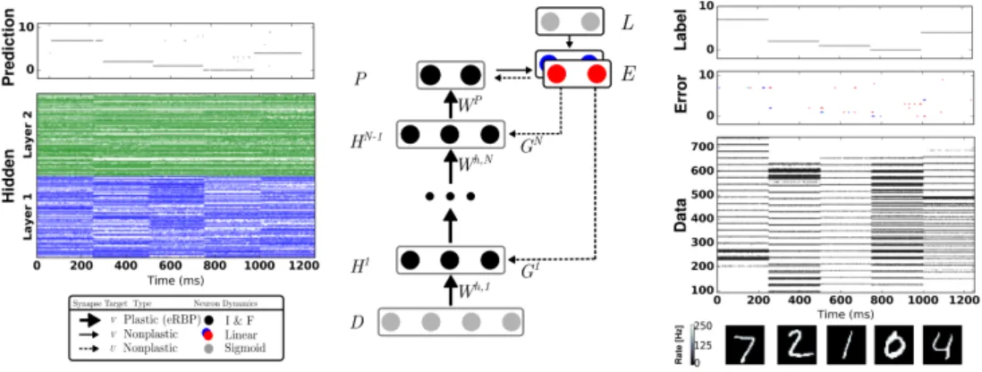
when an input spike occurs. ERBP solves the nonlocality problems, leading to remarkably good performance on MNIST handwritten digit recognition tasks (Fig. 8), achieving close to2%error compared to1.9%error using gradient backpropagation on the same network architecture.

One limitation event-driven Random Back-Propagation (eRBP) is related to the “loop duration”,i.e. the duration necessary from the input onset to a stable response in the error neurons. A related problem is layerwise locking in deep neural networks: because errors are backpropagated from the top layers, hidden layers must wait until the prediction is made available [Jaderberg et al., 2016]. This duration scales with the number of layers, limiting eRBP scalability for very deep networks. The loop duration problem is caused by the temporal dynamics of the spiking neuron, which are not taken into account in Eq. (19).

This problem can be partly overcome by maintaining traces of the input spiking activity, and a solution was reported in [Zenke and Ganguli, 2017]. Their rule, called Superspike is derived from gradient descent over the LI&F neuron dynamics, resulting in the following three-factor rule:

∆W_ijSS∝α∗(Erroriρ0(Ui)(pre∗Sj))) (20)

whereρdescribes the slope of the activation function ρat the membrane potentialUi, andprehere is the

response of the post-synaptic neuron to a pre-synaptic spike (the impulse response function atU).

Interestingly, both Eq. (20) and Eq. (19) rules are reminiscent of STDP but include further terms that vary according to some external modulation, itself related to some task. Unsurprisingly, the three terms in Eq. (18) can be related to the classical Widrow-Hoff (Delta) rule, where the first term is the error, the second is the derivative of the output activation function, and the third term is the input.

The loop duration is only partly solved with Eq. (20), as α and introduce memory of the previous activity into the synapses. However, this is only an approximation, as the dynamics of every layer leading to the top layer must be taken into account with one additional temporal convolution per layer. As a result, Eq. (20) and Eq. (19) do not scale well with multiple layers.

Figure 8: Network Architecture for Event-driven Random Backpropagation (eRBP). The network consists of feed-forward layers (784-200-200-10) for prediction and feedback layers for supervised training with labels (targets) L. Full arrows indicate synaptic connections, thick full arrows indicate plastic synapses, and dashed arrows indicate synaptic plasticity modulation. Neurons in the network indicated by black circles were implemented as two-compartment LI&F neurons. The top-layer errors are proportional to the difference between labels (L) and predictions (P) and is implemented using a pair of neurons coding for positive error (blue) and negative error (red). Each hidden neuron receives inputs from a random combination of the pair of error neurons. Output neurons receive inputs from the pair of error neurons in a one-to-one fashion. Reproduced from [Neftci et al., 2017a]

.

Local Errors A more effective method to overcome the loop duration and the layerwise locking problem is to use synthetic gradients: gradients that can be computed locally, at every layer. Synthetic gradients were initially proposed to decouple one or more layers from the rest of the network to prevent layerwise locking [Jaderberg et al., 2016]. Synthetic gradients usually involve an outer loop consisting of a full backpropagation through the network. While this provides convergence guarantees, a full backpropagation step cannot be done locally in spiking neural networks. Instead, relying on initialization of the local random classifier weights and forgoing the outer loop training yields good empirical results [Mostafa et al., 2017].

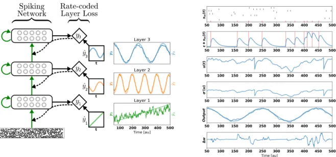
Using layerwise local classifiers [Mostafa et al., 2017], the gradients are computed locally using pseudo-targets (for classification, the labels themselves). To take the temporal dynamics of the neurons into account, the learning rule is similar to SuperSpike [Zenke and Ganguli, 2017]. However, the gradients are computed locally through a fixed random projection of the network activities into a local classifier. Learning is achieved using a local rate-based cost function reminiscent of readout neurons in liquid state machines [Maass et al., 2002], but where the readout is performed over a fixed random combination of the neuron outputs. The readout does not have a temporal convolution term in the cost function, the absence of which enables linear scaling, and does not prevent learning precise temporal spike trains (Fig. 9). The resulting learning dynamics are called DEep COntinuous Local LEarning (DECOLLE), and written:

∆W_ijDECOLLE ∝(X

k

gikErrork)ρ0(Ui)(pre∗Sj)). (21)

Here, the error is computed with respect to a random linear combination of the neuron outputs: Errork=

targetk−PigikSi. While SuperSpike scales at least quadratically with the number of neurons, learning with

local errors scales linearly [Kaiser et al., 2018]. Linearity greatly improves the memory and computational cost of computing the weight updates and simplifies potential RRAM implementations (see Sec. 5.2).

Independent Component Analysis with Three-Factor Rule Independent component analysis (ICA) is a very powerful tool to solve the cocktail party problem (blind source separation), feature extraction (sparse coding) and can be utilized in many applications such as de-noising images, Electroencephalograms (EEG) signals, and telecommunications [Hyvärinen, 2004]. ICA consists of finding mutually independent and non-Gaussian hidden factors (components), s, that form a set of signals or measurements, x. This problem can

Figure 9: Deep continuous local learning example. (Left) Each layer consists of spiking neurons with contin-uous dynamics. Each layer feeds into a local classifier through fixed, random connections (diamond-shaped, y). The classifier is trained to produce auxiliary targets yˆ. Errors in the local classifiers are propagated through the random connections to train the input weights, but no further (curvy, dashed line). To simplify the learning rule and enable linear scaling of the computations, the cost function is formulated using a rate code. The states of the spiking neurons (membrane potential, synaptic states, refractory state) are carried forward in time. Consequently, even in the absence of recurrent connections, the neurons are stateful in the sense of recurrent neural networks. (Right) Snapshot of the neural states illustrating the DECOLLE learning rule in the top layer. In this example, the network is trained to produce three time-varying pseudotargets

ˆ

y1,yˆ2 andyˆ3. Reproduced from [Kaiser et al., 2018]

be mathematically described for linearly mixed components as followsx=AswhereAis the mixing matrix. Both Aand s are unknowns. In order to find the independent components (sources), the problem can be formulated as u =Wx where x is the mixed signals (inputs of ICA algorithm), W is the weight matrix (demixing matrix),uis the outputs of the ICA algorithm (independent components). ICA’s strength lies in utilizing the mutual statistical independence of components to separate the sources.

Recently, Isomura and Toyoizumi have proposed a biological plausible learning rule called Error-Gated Hebbian Rule (EGHR)inspired from the standard Hebbian rule [Isomura and Toyoizumi, 2016] that enables local and efficient learning to find the independent components. The EGHR learning rule can be written as

∆WEHGR=ηh(Eo−E(u))g(u)xTi (22)

where η is the learning rate, h·i is the expectation over the ensemble (training samples), g(ui)xj is the

Hebbian learning rule, g(ui), xj are the postsynaptic and presynaptic terms of the neuron, respectively,

(Eo−E(u)) is the global error signal which consists of Eo which is a constant, and E(u) which is the

surprise or reward that guides the learning. The cost function of EGHR is defined asL=c1₂h(E0−E(u))2i.

It was proven mathematically and numerically that this learning rule is robust, stable and its equilibrium point is proportional to the inverse of the mixture matrix, i.e. the solution of ICA. This learning rule is a clear example of three-factor learning where the modulating is represented in the surprise,(Eo−E(u)). This

learning rule is a three-factor rule and can be performed using spiking neuron by following an implementation similar to [Savin et al., 2010].

ICA assumes that the sources are linearly mixed using a mixture matrixA. The final weight matrix,w, should converge tocA−1 which is still a valid solution sincec is a scaling factor. As previously discussed,

∆Gij can be replaced byη0∆wij to match the synaptic dynamics [Fouda et al., 2019], whereη0 is the scaled

learning rate, and∆wij is given by EGHR. Thus, the final equations for potentiation and depression pulses

can be written as follows:

∆nij|LT P ≈ 1 αP _η0_(E o−E(u))g(uj)xi Gmax−Gij(n) , and (23) ∆nij|LT D=− 1 αD _η0_(E o−E(u))g(uj)xi Gij(n)−Gmin , (24)

respectively. By programming the RRAMs using the previous equations, the circuit behaves as required and compensates for the asymmetric nonlinearity of the devices.

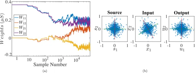
As a test bench for the proposed technique, we considered two Laplacian random variables that are generated and mixed using a mixture matrix which is set to a rotation matrixA= (cosθ,−sinθ; sinθ,cosθ)

with θ=π/6. Figure 10 shows the results of the online learning of independent components of the mixed signals. Figure 10a shows the weight evolution during the training. Clearly, there are some oscillations in the weights around the final solution after 104 _{samples because of the continuous on-line learning and the}

device variations. This can be avoided by using dynamic learning rate such as Adaptive Moment Estimation (Adam). A visual representation of the signals before mixing, after mixing and after training is shown in Fig. 10b which depicts the similarity between the source and output signals.

5

Stochastic Spiking Neural Networks

Up to now, we have considered fully deterministic neuron and synapse models. However, as discussed in Sec. 3.5.2, the writing (and in some cases, reading) of RRAMs values are stochastic. Additionally, analog VLSI neuron circuits have significant variability across neurons due to fabrication mismatch (fixed pattern noise) and behave stochastically due to noise intrinsic to the device operation. The variability at the device level can be taken in to account in SNN models and sometimes be exploited for improving learning performance and implementing probabilistic inference [Querlioz et al., 2015, Naous et al., 2016]. Here, we list avenues for implementing online learning in memory devices that exploit the stochasticity in the neurons and synapses.

A stochastic model of the neurons can be expressed as:

-0.2

0

0.2

0.4

1

₁₀

2

Sample Number

10

3

10

4

10

(a) -1 0 1 -1 0 1

Source

-1 0 1 -1 0 1

Input

-1 0 1 -1 0 1

Output

(b)

Figure 10: The online training results versus training time (a) Evolution of the weights, and (b) Visual results of the input and the output. Reproduced from [Fouda et al., 2019]

where ρi is the stochastic intensity (the equivalent of the activation function in artificial neurons), and η

and are kernels that reflect neural and synaptic dynamics, e.g. refractoriness, reset and postsynaptic potentials [Gerstner and Kistler, 2002]. The stochastic intensity can be derived or estimated experimentally if the noiseless membrane potential (Ui(t)) can be measured at the times of the spike [Jolivet et al., 2006].

This type of stochastic neuron model drives numerous investigations in theoretical neuroscience and forms the starting point for other types of adapting spiking neural networks capable of efficient communication [Zambrano and Bohte, 2016].

5.1

Learning in Stochastic Spiking Neural Networks

Neural and synaptic unreliability can induce the necessary stochasticity without requiring a dedicated source of stochastic inputs, for example, the unreliable transmission of synaptic vesicles in biological neurons. This is a well-studied phenomenon [Katz, 1966, Branco and Staras, 2009], and many studies suggested it as a major source of stochasticity in the brain [Faisal et al., 2008, Abbott and Regehr, 2004, Yarom and Hounsgaard, 2011, Moreno-Bote, 2014]. In the cortex, synaptic failures were argued to reduce energy consumption while maintaining the computational information transmitted by the post-synaptic neuron [Levy and Baxter, 2002]. More recent work suggested synaptic sampling as a mechanism for representing uncertainty in the brain, and its role in synaptic plasticity and rewiring [Kappel et al., 2015].

Strikingly, the simplest model of synaptic unreliability, a “blank-out” synapse, can improve the perfor-mance of spiking neural networks in practical machine learning tasks over existing solutions, while being extremely easy to implement in hardware [Goldberg et al., 2001], and often naturally occurring in emerging memory technologies [Saïghi et al., 2015, Al-Shedivat et al., 2015, Yu et al., 2013].

One approach to learning with such neurons and synapses is Event-Driven Contrastive Divergence (ECD), using ideas borrowed from Contrastive Divergence in restricted Boltzmann machines [Hinton, 2002]. The stochastic neural network produces samples from a probability distribution, and STDP carries out the weight updates according to the Contrastive Divergence rule in an online, asynchronous fashion. In terms of the three-factor rule above, ECD can be written:

∆W_ijECD=Mi(t)∆WijST DP (26)

where Mi(t) = 1 during the “data” phase andMi(t) = −1 during the “reconstruction” phase. These

neu-ral networks can be viewed as a stochastic counterpart of Hopfield networks [Hopfield, 1982], but where stochasticity is caused by multiplicative noise at the connections (synapses) or at the nodes (neurons).

ECD requires symmetric weights, which is difficult to achieve due to the weight transport problem discussed above. A variation of ECD called random Contrastive Hebbian learning (rCHL) [Detorakis et al., 2018a], replaces the transpose of the synaptic weights with fixed random matrices. This was performed similarly to Feedback Alignment (FDA) [Lillicrap et al., 2016]. Contrastive Hebbian Learning (CHL) is similar to Contrastive Divergence, but it employs continuous nonlinear dynamics at the neuronal level. Like

Figure 11: The Synaptic Sampling Machines (SSM). (a) At every occurrence of a pre-synaptic event, a pre-synaptic event is propagated to the post-synaptic neuron with probabilityp. (b) Synaptic stochasticity can be viewed as a continuous DropConnect method [Wan et al., 2013] where weights are masked by a binary matrix Θ(t), where ∗ denotes element-wise multiplication. (c) SSM Network architecture, consisting of a visible and a hidden layer. Reproduced from [Neftci et al., 2016]

.

Contrastive Divergence, it does not rely on a special circuitry to compute gradients (but can be interpreted as the gradient of an objective function), allows information to flow in a coupled, synchronous way, and is grounded upon Hebb’s learning rule. CHL uses feedback to transmit information from the output layer to hidden(s) layer(s), and in instances when the feedback gain is small (such as in the clamped phase), has been demonstrated by Xie and Seung to be equivalent to Backpropagation [Xie and Seung, 2003]. Using this approach, the information necessary for learning propagates backward, though it is not transmitted through the same axons (as required in the symmetric case), but instead via separate pathways or neural populations. Equilibrium Propagation (EP) describes another modification of CHL that generalizes the objective functions it can solve and improve on its theoretical groundings. In EP the neuron dynamics are derived from the energy function, however, EP requires symmetric weights. The energy function used in Equilibrium Propagation includes a mean-squared error term on the output units, allowing the output to be weakly clamped to the true outputs. (e.g. labels). The neuron model takes a form which is reminiscent of the LI&F neuron. The recurrent dynamics in the network affect the other layers in the network, similarly to CHL. Both rCHL and EP were formulated for continuous (rate-based) neurons, although their implementation with spikes is straightforward following the same approach as SSMs.

Learning in stochastic neuron networks can also be performed using the surrogate gradient approach and three-factor rules. In this case, a simple approach is to use the stochastic intensityρas a drop-in replacement of the neural activation function for purposes of computing the weight updates [Neftci et al., 2019]. In this case, stochasticity plays a regularization role similar to dropout in deep learning [Neftci et al., 2017b] and weight normalization [Neftci, 2017] an online modification of batch normalization.

5.2

Three Factor Learning in Memristor Arrays

So far, we have discussed how to implement gradient-based learning as local synaptic plasticity rules in SNNs. In many cases, gradient-based learning provides superior results compared to STDP and take the form of three-factor rules. These rules are biologically credible since pre- and post-synaptic activities are available at the level of the neuron and neurotransmitters in the brain can carry the extrinsic factor. However, besides the LTP and LTD asymmetry problems already discussed, the implementation of the three-factors in memristor arrays come with certain challenges. The first challenge concerns the implementation of the synaptic traces.

In certain simple cases, such as when the subthreshold neural dynamics are linear, only one trace for each neuron involved in the learning connections is required for learning [Kaiser et al., 2018], similar to the STDP case. Previous work has demonstrated STDP learning in RRAM and hence capture some form of a neural trace. The majority of these include additional CMOS circuitry in a “hybrid configuration” [Ielmini, 2018] to enable STDP. The simplest of these implementations consists of a 2T1R configuration that enables an update when both terminals are high (both spike). While this is sufficient for the case whereα=β= 0, an additional mechanism that filters the spike is necessary to recover STDP like curves whenα >0or β >0. This can be achieved with a circuit that is similar to that of the synapse [Bartolozzi and Indiveri, 2008] or calcium variables [Mitra et al., 2006]. For more complex neuron dynamics (such as non-linear neuron dynamics), then at least one trace per synapse is required, [Bellec et al., 2019], and ideally, one trace per connection and per neuron [Williams and Zipser, 1989].

Since the synaptic trace dynamics follow similar first order (RC) dynamics, the same circuits used to implement first-order synaptic dynamics can be used to implement synaptic traces [Bartolozzi and Indiveri, 2006] or dedicated calcium dynamics circuits [Huayaney et al., 2016]. However, scalability can become an issue: the same amount of memory for storing the weights is necessary for computing the traces, but the latter must be carried out continuously. One potential solution comes from recent work in using diffusive memristors to implement the leaky dynamics of integrate and fire neurons [Wang et al., 2018], which can be used for computing neural traces.

The second issue concerns the modulation. In many gradient-based three-factor rules, the modulation of the learning rule is specific to each neuron, not each synapse. This means that a similar approach to eRBP Eq. (19), where a separate neuron compartment is used for maintaining the modulation factor can in principle be used in memristor arrays,i.e. the weight update can consist in the two factors(pre∗Sj)),

whereMiρ0(Ui).

Additionally, the variability in the conductance reading and writing can cause the learning to fail or slow down. Independent noise in the read or write is not a problem and can even help learning, as discussed in the stochastic SNN section. Fixed pattern noise, however, can be problematic as it translates into variable learning rates per weight and can impair learning.

6

Concluding Remarks

In this chapter, we presented neural and synaptic models for learning in spiking neural networks. In particu-lar, we focused on synaptic plasticity models that use approximate gradient-based learning that is potentially compatible with a neuromorphic implementation and memristor arrays. Gradient-based learning in spiking neural networks generally provide the best performances on many applications, such as image recognition, probabilistic inference, and ICA. The mathematical modeling of the synaptic plasticity revealed that these dynamics take the form of three-factor rules, which can be viewed as a type of modulated Hebbian learning. While Hebbian learning or its spiking counterpart, STDP have been previously demonstrated in memristors, three-factor rules also require modulation of the learning at the postsynaptic neurons. Furthermore, if the neuron and synapse model are equipped with temporal dynamics, then it may become necessary to maintain pre-synaptic and post-synaptic activity traces in the crossbar to address the temporal credit assignment problem. Through the mathematical models, we identified which approaches are viable for implementing the modulation and the neural traces with memristors.

References

L.F. Abbott and W.G. Regehr. Synaptic computation. Nature, 431:796–803, October 2004.

M Al-Shedivat, R. Naous, E. Neftci, G. Cauwenberghs, and K.N. Salama. Inherently stochastic spiking neurons for probabilistic neural computation. In IEEE EMBS Conference on Neural Engineering, Apr 2015.

Renzo Andri, Lukas Cavigelli, Davide Rossi, and Luca Benini. Yodann: An ultra-low power convolutional neural network accelerator based on binary weights. In2016 IEEE Computer Society Annual Symposium on VLSI (ISVLSI), pages 236–241. IEEE, 2016.

Navin Anwani and Bipin Rajendran. Normad-normalized approximate descent based supervised learning rule for spiking neurons. In Neural Networks (IJCNN), 2015 International Joint Conference on, pages 1–8. IEEE, 2015.

M Azzaz, E Vianello, B Sklenard, P Blaise, A Roule, C Sabbione, S Bernasconi, C Charpin, C Cagli, E Jalaguier, et al. Endurance/retention trade off in hfox and taox based rram. In 2016 IEEE 8th International Memory Workshop (IMW), pages 1–4. IEEE, 2016.

C. Bartolozzi and G. Indiveri. Silicon synaptic homeostasis. In Brain Inspired Cognitive Systems, BICS 2006, pages 1–4, October 2006.

C. Bartolozzi and G. Indiveri. Synaptic dynamics in analog VLSI. Neural Computation, 19(10):2581–2603, Oct 2007. doi: 10.1162/neco.2007.19.10.2581.

C. Bartolozzi and G. Indiveri. A silicon synapse implements multiple neural computational primitives. The Neuromorphic Engineer, 2008.

Guillaume Bellec, Franz Scherr, Elias Hajek, Darjan Salaj, Robert Legenstein, and Wolfgang Maass. Biolog-ically inspired alternatives to backpropagation through time for learning in recurrent neural nets. arXiv preprint arXiv:1901.09049, 2019.

Ben Varkey Benjamin, Peiran Gao, Emmett McQuinn, Swadesh Choudhary, Anand R Chandrasekaran, J Bussat, Rodrigo Alvarez-Icaza, John V Arthur, PA Merolla, and Kwabena Boahen. Neurogrid: A mixed-analog-digital multichip system for large-scale neural simulations. Proceedings of the IEEE, 102(5): 699–716, 2014.

G-Q. Bi and M-M. Poo. Synaptic modifications in cultured hippocampal neurons: Dependence on spike timing, synaptic strength, and postsynaptic cell type. J. Neurosci., 18(24):10464–10472, 1998.

Sander M Bohte, Joost N Kok, and Johannes A La Poutré. Spikeprop: backpropagation for networks of spiking neurons. InESANN, pages 419–424, 2000.

Tiago Branco and Kevin Staras. The probability of neurotransmitter release: variability and feedback control at single synapses. Nature Reviews Neuroscience, 10(5):373–383, 2009.

Chih-Cheng Chang and et al. Mitigating asymmetric nonlinear weight update effects in hardware neural network based on analog resistive synapse. IEEE Journal on Emerging and Selected Topics in Circuits and Systems, 2017.

B Chen, Y Lu, B Gao, YH Fu, FF Zhang, P Huang, YS Chen, LF Liu, XY Liu, JF Kang, et al. Physical mechanisms of endurance degradation in tmo-rram. In2011 International Electron Devices Meeting, pages 12–3. IEEE, 2011.

E. Chicca, F. Stefanini, and G. Indiveri. Neuromorphic electronic circuits for building autonomous cognitive systems. Proceedings of IEEE, 2013.

Matthieu Courbariaux, Yoshua Bengio, and Jean-Pierre David. Low precision arithmetic for deep learning.

arXiv preprint arXiv:1412.7024, 2014.

Matthieu Courbariaux, Itay Hubara, Daniel Soudry, Ran El-Yaniv, and Yoshua Bengio. Binarized neural networks: Training deep neural networks with weights and activations constrained to+ 1 or-1. arXiv preprint arXiv:1602.02830, 2016.

M. Davies, N. Srinivasa, T. H. Lin, G. Chinya, P. Joshi, A. Lines, A. Wild, and H. Wang. Loihi: A neuromorphic manycore processor with on-chip learning.IEEE Micro, PP(99):1–1, 2018. ISSN 0272-1732. doi: 10.1109/MM.2018.112130359.

Georgios Detorakis, Travis Bartley, and Emre Neftci. Contrastive hebbian learning with random feedback weights. Neural Networks, 2018a. URLhttps://arxiv.org/abs/1806.07406. (accepted).