Field validation and benchmarking of a cloud shadow
speed sensor
P. Kuhn1,∗
Paseo de Almería 73, 04001 Almería, Spain
M. Wirtz1, S. Wilbert1, J. L. Bosch2, G. Wang3, L. Ramirez4, D. Heinemann5,
R. Pitz-Paal6
Abstract
With ramp rate regulations for photovoltaic plants being discussed in many countries, the speed of clouds has gained signicant importance lately. Besides, measuring cloud velocities and directions is of interest for validations of nu-merical weather predictions and solar nowcasting systems. Recently, the Cloud Shadow Speed Sensor (CSS) was developed and validated in San Diego for low cumulus clouds. In this publication, the CSS is studied under dierent weather and cloud conditions in the desert of Tabernas in southern Spain. Furthermore, a novel shadow camera based low-cost, low-maintenance approach to determine cloud shadow motion vectors is presented and used as a reference to benchmark the CSS. In comparison, the absolute velocities derived from the CSS and the shadow camera on 59 days for ±5 min temporal medians show deviations of
∗Corresponding author
Email address: [email protected] (P. Kuhn)
1German Aerospace Center (DLR), Institute of Solar Research, Paseo de Almería 73, 04001
Almería, Spain.
2Departamento de Ingeniería Eléctrica y Térmica, Universidad de Huelva, Campus de La
Rábida, Carretera de Palos de la Frontera S/N 21071 La Rábida, Palos de la Frontera (Huelva)
3Dept of Mechanical and Aerospace Engineering, UCSD Center for Energy Research,
Uni-versity of California, 92093-0411 La Jolla, USA.
4CIEMAT, Energy Department - Renewable Energy Division. Av. Complutense, 40, 28040
Madrid, Spain.
5Energy Meteorology Unit, Energy and Semiconductor Research Laboratory, Institute of
Physics - Oldenburg University, 26111 Oldenburg, Germany.
6German Aerospace Center (DLR), Institute of Solar Research, Linder Höhe, 51147
RMSD 2.1 m/s (28.0 %), MAD 1.2 m/s (15.7 %) and a bias of -0.2 m/s (2.8 %). Deviations of the cloud shadow direction are RMSD47.9° (26.6 %), MAD25.3°
(14.0 %) and bias3.7° (2.0 %). An adaption of the CSS software yields 91 %
more measurements on 59 days in comparison to the previously used algorithms at the expense of reduced accuracies, both for the measured velocities and for the measured directions.
The CSS and the novel shadow camera based reference system enable long-time, low-maintenance ground measurements of cloud shadow speeds, which were previously not available. The distinct advantages and limitations of the two systems are discussed. In addition to the comparisons between the shadow camera system and the CSS on 59 days, the detection rates of the CSS are classied and measured on 223 days by analyzing CSS radiometer signals. De-pending on the shading strength and shading durations, detection rates vary between 3.7 % and 21.6 %. Furthermore, the basic assumption as well as pos-sible correction approaches of the linear cloud edge - curve tting method are studied.
The CSS was found to be a robust tool with great potential. However, optically thin clouds with diuse edges pose a challenge and the detection rate leaves room for improvements. The newly developed shadow camera system provides more measurements which scatter less but needs certain geographical requirements. The shadow camera is found to be a feasible validation tool for cloud (shadow) motion vectors.
Keywords: Cloud shadow speed sensor, cloud speed, shadow camera system 1. Introduction
1
Obtaining reference motion vectors of clouds is relevant for the optimization
2
and validation of all-sky imager based nowcasting systems (Kuhn et al., 2017a)
3
as well as numerical weather predictions (NWP) and satellite-based weather
4
forecasts (Molteni et al. (1996), Klein and Jakob (1999), Tomassini et al. (1999)).
5
In addition to that, the rapid growth of solar power generation with its inherent
variability calls for solar forecasting tools, which can predict shading events.
7
Recently, ramp rate regulations (Lave et al. (2013), Marcos et al. (2014), Chen
8
et al. (2017)) in several countries with high solar grid penetrations have further
9
stressed the need of cloud speed measurements. The Cloud Shadow Speed
10
Sensor (CSS) can be used to derive such cloud motion vectors and can be a part
11
of a camera-based solar nowcasting system (Wang et al., 2016). A singular
all-12
sky imager can measure angular speeds of clouds, but cannot provide absolute
13
speeds in [m/s].
14
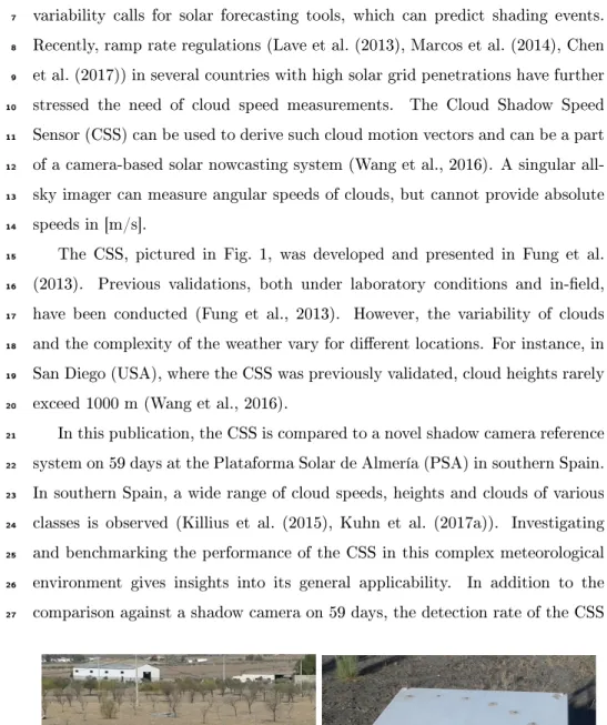
The CSS, pictured in Fig. 1, was developed and presented in Fung et al.
15
(2013). Previous validations, both under laboratory conditions and in-eld,
16
have been conducted (Fung et al., 2013). However, the variability of clouds
17
and the complexity of the weather vary for dierent locations. For instance, in
18
San Diego (USA), where the CSS was previously validated, cloud heights rarely
19
exceed 1000 m (Wang et al., 2016).
20
In this publication, the CSS is compared to a novel shadow camera reference
21
system on 59 days at the Plataforma Solar de Almería (PSA) in southern Spain.
22
In southern Spain, a wide range of cloud speeds, heights and clouds of various
23
classes is observed (Killius et al. (2015), Kuhn et al. (2017a)). Investigating
24
and benchmarking the performance of the CSS in this complex meteorological
25
environment gives insights into its general applicability. In addition to the
26
comparison against a shadow camera on 59 days, the detection rate of the CSS
27
(a) (b)
is determined on 223 days by directly investigating the measurements of the
28
CSS sensors.
29
The shadow camera is a downward-facing camera placed on top of an 87 m
30
high tower (CIEMAT CESA-I), which is part of a shadow camera system
pro-31
viding spatially resolved irradiance maps (Kuhn et al. (2017a), Kuhn et al.
32
(2017b), Kuhn et al. (2017c), Kuhn et al. (2018a)). The shadow camera is used
33
to measure reference cloud speeds, which are compared to the CSS.
34
This publication is structured as follows. After the introduction, the CSS is
35
presented and its software optimization discussed in section 2. In section 3, the
36
shadow camera method is explained in detail. Comparing these two systems
37
in section 4 enables an in-eld validation of the CSS. Also, the detection rate
38
is determined in this section by scrutinizing the raw data of the CSS. The
39
advantages and disadvantages of the CSS in comparison with the shadow camera
40
approach are discussed in section 5. The conclusion is given in section 6. In
41
the appendix, assumptions and possible corrections of the Linear Cloud Edge
42
method are studied.
43
2. The Cloud Shadow Speed Sensor
44
2.1. Working principle
45
The working principle of the CSS, developed by Fung et al. (2013), is based
46
on methods for determining cloud motion vectors with an array of irradiance
47
sensors (Bosch and Kleissl (2013), Bosch et al. (2013), Schenk et al. (2015)). It
48
consists of nine uncalibrated photodiode pyranometers, which are sampled at
49
a frequency of 667 s−1. Eight of these sensors are placed in a circular arc of
50
105° with a radius of 29.7 cm around the ninth sensor (see Fig. 1). In order to 51
measure the speed and direction of a cloud shadow, the CSS must be directly
52
shaded. If the shadow of a cloud passes the CSS, the sensors detect ramps at
53
slightly dierent times. This way, both the speed and the direction of the clouds
54
is determined. Due to the high frequency, the distances of the sensors can be
small, which enabled a very compact design. Overall material costs are specied
56
to be approximately 400 US-$ (Wang et al., 2016).
57
The CSS does not need regular cleaning as the working principle is based on
58
relative deviations, not absolute irradiance measurements. As experienced over
59
more than two years of active service, this user-friendly maintenance routine was
60
found to hold even in the harsh conditions of the desert of Tabernas (Almería,
61
Spain). Although not cleaned, the CSS data are checked daily, e.g. to detect
62
constantly shaded sensors due to bird excrements. Luckily, such an event did
63
not occur yet. Based on this dierential approach, the CSS is able to determine
64
the motion vectors of cloud shadows, not directly the motion vectors of the
65
clouds. However, these vectors deviate only insignicantly (Fung et al., 2013).
66
2.2. Software adaptions of the CSS
67
During this comparison campaign, no hardware adjustments were conducted
68
on the CSS. Suggestions for hardware improvements are mentioned in the
con-69
clusion. However, the evaluation method of the CSS is scrutinized and adapted.
70
All comparisons to the shadow camera measurements will be conducted on the
71
CSS with and without these adaptions.
72
Increasing the detection rate
73
In the rst step of the evaluation algorithm, the CSS lters its data and it
74
does not provide cloud speed measurements if certain criteria are not met. In
75
any case, however, the raw data is stored. The ltering as implemented in Fung
76
et al. (2013) and Wang et al. (2016) is based on a second order error metric
77
(presented in the following), which results in a low number of calculated cloud
78
motion vectors in relation to the total number of shading events.
79
The algorithm used for the cloud motion measurements itselves and
de-80
scribed in Wang et al. (2016) is the LCE - curve tting algorithm, which
deter-81
mines the maximum cross-correlation coecientRij of each pair of signals and 82
records the associated time shift ∆ti,j for the sensor pair consisting of sensor 83
iand j corresponding to this maximum cross-correlation. Due to the setup of
v D cos( φ− δ3) D S0
Approaching cloud shadow
S1 S3 S5
φ δ3
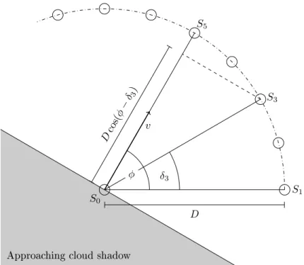
Figure 2: Depicted in the bottom-left corner is a shadow approaching the CSS with a speed
vand a directionφ. SensorS0 is shaded rst, sensorS1 is shaded Dvcos(φ)afterS0. Then sensorS3 is shaded Dvcos(φ−δ3)andS5 Dv afterS0. Based on these time dierences, the motion vector of the shadow can be calculated.
the CSS, there are#(i◦j) = #α= 12sensor pairs. Based on the time shifts of 85
these sensor pairs, the speed is calculated. The method will be briey described
86
here and is explained in detail in Wang et al. (2016).
87
In Fig. 2, an example situation is shown. Coming from the bottom-left, a
88
shadow is sequentially shading the sensors. The trigonometric relation visualized
89
in Fig. 2 holds for all cloud edge directions as the cloud speed is assumed to be
90
perpendicular to the cloud edge. Deviations caused by this this assumption are
91
studied in section A.
92
The residuum of the cosine tΓacts as a lter (equ. 1). 93 Γ = 1− P12 α=1(tα,F it(φ, v)−tα)2 t (1) 94
It is calculated withtα,F it(φ, v)being the time shift according to the calculated 95
cosine t,tαbeing the measured time shift andtRM Sbeing the quadratic scatter 96
of the time shifts according to equ. 2.
97 tRM S = 12 X α=1 (tα− 1 12 12 X α=1 tα)2 (2) 98
If the average of the maximum cross-correlation coecientsRij is less than 0.9 99
or the residuum Γ of the cosine curve t is less than 0.9, the cloud motion 100
vector will not be computed. A small Rij is likely a result of an erroneous 101
measurement or dynamically changing clouds. Similar, a smallΓindicates poor 102
curve tting and therefore an unreliable result. Based on these two criteria,
103
measurements are rejected. The calculation of the cosine t is based on a least
104
square approach (LSQ). This approach, presented in Wang et al. (2016), is
105
highly sensitive towards outliers and thus rejects many measurements.
106
In order to reduce the inuence of outliers towards the cosine t, several
107
regression models such as the least square method (LSQ, Wang et al. (2016)), the
108
least absolute deviation method (LAD, Bloomeld and Steiger (2012)), the least
109
trimmed squares method (LTS, Giloni and Padberg (2002), Mount et al. (2014))
110
and the least median of squares method (LMS, Rousseeuw (1984)) were studied.
111
All methods are discussed in detail in the literature (Rousseeuw and Croux
112
(1993), Huber (2009)) and will not be introduced here. Considering 347023
113
measuring intervals on 223 days, the LSQ method obtains 5830 cloud motion
114
vectors (speed and direction). The LAD method obtains 8034, the LTS method
115
17334 and the LMS method 21535 motion vectors. The LTS method is found
116
to have the least deviations in comparison to the LSQ method and yields 197 %
117
more measurements on 223 days (91 % more measurements on the 59 days which
118
could be temporally matched to shadow camera measurements as considered in
119
section 4.2 and section 4.3). The CSS measurements derived from both the
120
LSQ and the LTS method will be compared to shadow camera measurements.
121
In section 4.4, the determination of the detection rate is presented.
122
Lowering the thresholds of the LSQ method can also be used to obtain more
123
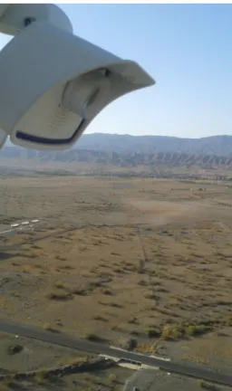
Figure 3: One of the six shadow cameras overlooking the PSA from top of a tower (CIEMAT CESA-I), 87 m above the ground.
compared to the shadow camera measurements.
125
3. The shadow camera reference
126
The shadow camera measures cloud motion vectors (speeds and directions)
127
by comparing three concurrent images. It is based on one o-the-shelf
surveil-128
lance camera (Mobotix MX-M24M-Sec-D22, CMOS sensor) and located on a
129
87 m high tower (CIEMAT CESA-I, Fig. 3 displays a shadow camera).
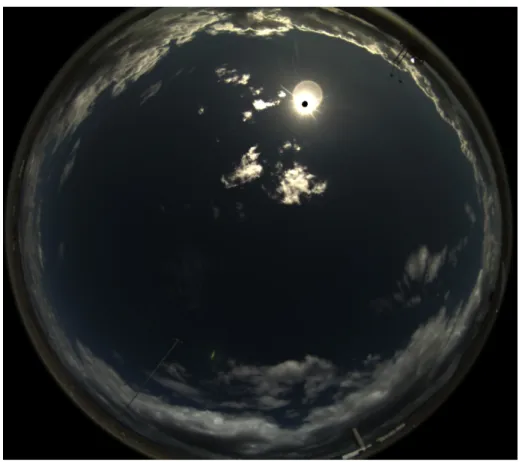
Ev-130
ery 15 s, an 8 bit RGB image of 2048 ×1536 pixels is taken (Fig. 4a). Using
131
both the determined interior (using methods described in Scaramuzza et al.
132
(2006)) and external (via GPS reference points) orientation, an orthoimage is
133
calculated (Fig. 4b). In this orthoimage, the dimensions of all pixels are known
Figure 4: Left: raw image of the used shadow camera. The arrow marks the position of the CSS. Right: undistorted raw image as projected on a ground model. The star marks the position of the CSS. The white frame depicts the 525 m×525 m large area in which cloud
shadow speeds are determined.
in [m]. From three concurrent orthoimages and a novel dierential approach,
135
cloud speeds and cloud directions are resolved. Due to the viewing geometry,
136
pixels imaging areas far away from the camera's position are distorted (see e.g.
137
bottom-left in Fig. 4b). In order to derive robust cloud motion vectors, only a
138
quadratic area of 105× 105 pixels (525 m×525 m) within the orthoimage is
139
considered.
140
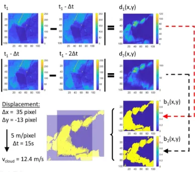
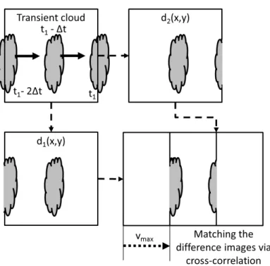
The approach to derive cloud (shadow) motion vectors is visualized in Fig. 5.
141
Three subsequent cropped orthoimages corresponding to the timestamps t, t-∆t
142
and t-2∆tare converted to grayscale and two dierence images di are derived. 143
The rst dierence imaged1is the absolute of the subtraction of the image t and
144
image t-∆t. The second dierence image d2 is the absolute of the subtraction
145
of the images t-∆t and t-2∆t. The approach is given in equ. 3 and equ. 4
146
with∆t being 15 s. xand yare the pixel coordinates in the cropped grayscale
147 orthoimagesimortho. 148 d1(x, y) =imortho(x, y, t)−imortho(x, y, t−∆t) (3) 149 150 d (x, y) =im (x, y, t−∆t)−im (x, y, t−2∆t) (4)
Figure 5: Shadow camera deriving cloud motion vectors: from three subsequent cropped and grayscale-converted orthoimages, dierence imagesdiare calculated. Via an empirically found threshold, binary dierence images bi are derived. These two dierence images are then matched using cross-correlation. For the example situation depicted here (2016-12-01, 14:15:15 h - 14:15:45 h, UTC+1), a displacement of∆x= 35 pixel and∆y =−13pixel is calculated. This corresponds to a shadow velocity of 12.4 m/s.
The dierence images are converted into binary images bi by an empirically 152
found threshold (dashed arrows in Fig. 5). The pixel displacements∆xand∆y
153
between the two binary dierence imagesbi is obtained by the normalized 2-D 154
cross-correlation approach presented in Huang et al. (2012) (see Fig. 5, bottom
155
row). From the displacement vector, the cloud shadow speed can be derived
156 using equ. 5. 157 v= p (∆x)2+ (∆y)2 ∆t ×kSC (5) 158
Caused by technical limitations, the shadow camera can reliably resolve
159
cloud motion vectors up to 17.5 m/s. The limiting factor is a result of the
160
temporal resolution of∆t= 15 s. This image acquisition rate is chosen to limit
161
the amount of produced data. The camera itself can take up to 25 images per
Figure 6: Visualization of the maximum resolvable velocityvmax: due to storage limitations, imposing a low image acquisition rate, the used shadow camera can reliably resolve cloud motion vectors up to 17.5 m/s.
second. The maximum velocity is calculated with equ. 6 and visualized in Fig. 6.
163 164 vmax= N kSC 2∆t = 17.5 m/s (6) 165
Equation 6 is derived by looking at a cloud crossing the area under consideration
166
in parallel to its borders (see Fig. 6). The quadratic imaged area has edge lengths
167
of N kSC = 105pixel·5 m/pixel = 525 m. A cloud entering the imaged area 168
at timet−2∆t and leaving it at time t results in a rst (absolute) dierence
169
imaged1with detected movements at a border and in the center. Similarly, the
170
second dierence imaged2 detects movements in the center and at the adjacent
171
border. The matching via cross-correlation eectively divides the area by two,
172
which this way denes the maximum resolvable velocityvmax. 173
The eects of this limitation will be discussed in section 4. In order to
detect cloud (shadow) movements, the shadow camera needs an reasonably
ho-175
mogeneously area with little non-cloud movements and an elevated position for
176
feasible viewing geometries. In Kuhn et al. (2018b), a system consisting of a
177
shadow camera and an all-sky imager for cloud height determinations is
pre-178
sented. Further applications of shadow cameras are discussed in Kuhn et al.
179
(2017b).
180
To investigate the cloud motion vectors, each CSS measurement, without
181
any temporal averaging, is compared to the±2 min (four-minute) median of the
182
shadow camera measurements. Furthermore,±2 min (four-minute) and±5 min
183
(ten-minute) medians of the CSS measurements are compared to corresponding
184
shadow camera measurements. If within the individual temporal interval no
185
reference measurement is available, the corresponding CSS measurements are
186
dropped. As the shadow camera approach derives reliably velocities only up
187
to 17.5 m/s, CSS measurements with a corresponding reference value above
188
this speed are also dropped. For the investigation of cloud motion directions,
189
vectors measured by the CSS and the shadow camera are compared to each
190
other. Without the temporal averaging, the LSQ method is studied on 2956
191
measurements and the LTS method on 4828 measurements for which shadow
192
camera reference measurements are available. In total, the LSQ method derived
193
3170 measurements on 59 days, the LTS method 6041 and the shadow camera
194
23155. To quantify the deviations, root-square deviations (RMSD),
mean-195
absolute deviations (MAD) and the bias are calculated (equ. 7-9).
196 RMSD= v u u t 1 N N X i=1 (vCSS,i−vSC,i)2 (7) 197 198 MAD= 1 N N X i=1 |vCSS,i−vSC,i| (8) 199 200 bias= 1 N N X i=1 (vCSS,i−vSC,i) (9) 201
4. Benchmarking the CSS
202
In section 2.2, an algorithmic change in the software of the CSS is discussed,
203
which signicantly increases the amount of detected shading events. In this
204
section, both approaches (LSQ and LTS, see section 2.2) are compared to the
205
shadow camera reference measurements. To begin with, three example days are
206
studied in detail in section 4.1. In section 4.2, cloud shadow speed measurements
207
are studied on 59 days. The directions of the cloud shadows are compared to
208
shadow camera measurements in section 4.3. The detection rate of the CSS is
209
investigated based on its radiometer measurements on 223 days in section 4.4
210
(not in comparison to the shadow camera). After focussing on the deviations
211
found with the LSQ approach, the deviations of the LTS approach, yielding
212
more measurements, are discussed in section 4.5.
213
The speed distributions as measured by the CSS and the shadow camera is
214
depicted in Fig. 7. In the top left, the overall number of occurrence is shown.
215
The shadow camera obtains far more measurements than the CSS, for which
216
the LTS method yields more results than the LSQ method. The vertical line
217
marks the maximum speed reliably resolvable by the shadow camera (17.5 m/s,
218
see section 3). This limit was derived for a worst case scenario. Cloud
shad-219
ows moving diagonally over the imaged area can be reliably measured up to
220
17.5 m/s·√2 = 24.7 m/s. In extreme cases, diagonal cloud shadow speeds up 221
to 525 m/15s·√2 = 49.5 m/s can be measured. However, beyond 17.5 m/s, 222
the speeds cannot be safely resolved for all directions. 92.6 % of all shadow
223
camera measurements are below 24.7 m/s, 81.4 % of all shadow camera
mea-224
surements are below 17.5 m/s. 92.1 % of all CSS measurements obtained with
225
the LSQ method are below 17.5 m/s (98.5 % below 24.7 m/s). 93.0 % of all
226
CSS measurements derived with the LTS method are below 17.5 m/s (98.1 %
227
below 24.7 m/s). Given the distribution of the speeds measured by the CSS
228
and the limitations of the shadow camera, all shadow camera measurements
229
beyond 17.5 m/s are excluded from the comparisons in this section. For speeds
230
considered in the following comparisons (v <= 17.5 m/s), the mean speed of 231
Figure 7: Top left: histograms of all cloud motion vectors obtained on 59 days by the shadow camera (SC), the CSS using the LSQ method (LSQ) and the CSS using the LTS method (LTS). Top right: relative frequency of occurence. Bottom left: bin-wise subtraction of the number of occurrence (see top left). Bottom right: bin-wise subtraction of the relative frequency of occurrence (see top right). The vertical line marks the maximum speed reliably resolvable by the shadow camera for all cloud motion directions.
the shadow camera measurements is 7.36 m/s (median: 6.67 m/s), the mean
232
speed of the CSS measurements with the LSQ approach is 8.99 m/s (median:
233
7.69 m/s) and with the LTS approach 8.60 m/s (median: 7.30 m/s). Although
234
the modes of the histograms are at 6.0 m/s, a wide range of cloud speeds are
235
measured.
236
4.1. Three example days
237
Before looking at long-term comparisons in the next sections, three example
238
days are specically studied. The example days are 2016-03-19, 2016-04-22
239
and 2016-10-14. For these example days, the CSS data are shown without any
240
temporal averaging. The eects of temporal averaging on the comparisons are
241
studied in the next sections.
242
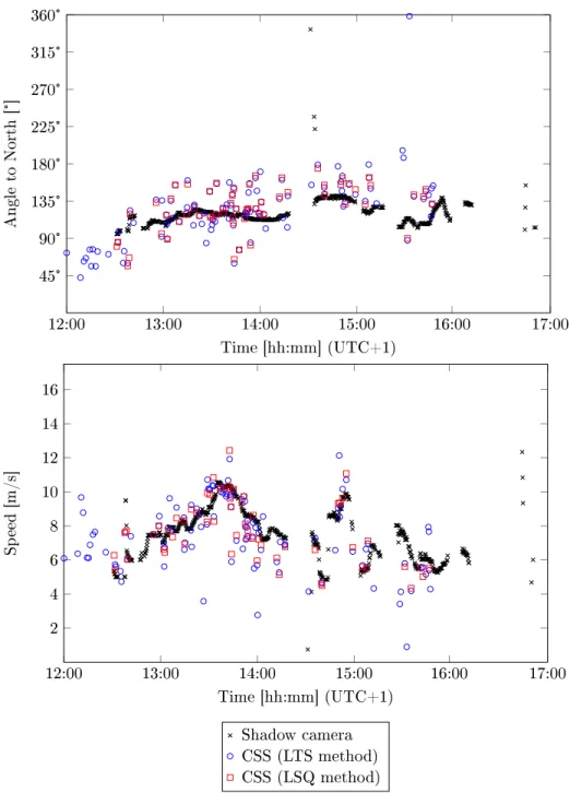
The cloud speeds and direction of 2016-10-14 are shown in Fig. 9. Cloud
mo-243
tion directions are displayed in the top part, cloud velocities in the bottom part.
Figure 8: All-sky image taken at 2016-10-14, 12:10:00 UTC+1. Small clouds are visible around the sun, which are dynamically forming.
The values of the reference system are depicted as ±2 min medians; the CSS
245
measurements are not additionally averaged or ltered. On this day,
altocumu-246
lus clouds between 2000 and 3000 m are predominant, traveling from north-west
247
to south-east. The shadow camera obtained 653 measurements on this day, the
248
CSS with the LSQ method 60 and with the LTS method 111 measurements.
249
Prior to 12:31 h (UTC+1), the shadow camera does not provide
measure-250
ments. Looking at the shadow camera video of this day, the lack of
measure-251
ments can be explained by a lack of (visible) shading events. The shading events
252
measured by the CSS are not visible in the shadow camera video. However, the
253
data of a near-by all-sky imager show that around 12:15 h there are some tiny
12:00 13:00 14:00 15:00 16:00 17:00 45° 90° 135° 180° 225° 270° 315° 360° Time [hh:mm] (UTC+1) Angle to North [°] 12:00 13:00 14:00 15:00 16:00 17:00 2 4 6 8 10 12 14 16 Time [hh:mm] (UTC+1) Sp eed [m/s] Shadow camera CSS (LTS method) CSS (LSQ method)
Figure 9: CSS and shadow camera measurements on 2016-10-14. The shadow camera reference measurements show less scatter than the CSS measurements.
clouds dynamically forming around the sun (see Fig. 8). This might be an
ex-255
ample of a nugget eect with the spatial resolution of the CSS being far higher
256
than the spatial resolution of the shadow camera at the position of the CSS.
257
This eect and its impact on these comparisons are discussed later and partially
258
compensated by temporal averaging later-on.
259
Between 12:30 h (UTC+1) and 14:30 h, the measured velocities increase from
260
approximately 5 m/s to 10 m/s and decrease back to approximately 6 m/s. Later
261
that day, large scattered clouds with dierent velocities are present. For this
262
day, the CSS measurements and the reference system align very well. Ceilometer
263
data and all-sky imager videos show that there is only one cloud layer present.
264
The deviation found on this day for the LSQ and the LTS method are displayed
265
in Tab. 1.
Table 1: Deviations between the LSQ and LTS approach in comparison to the shadow cam-era on 2016-10-14. Instantaneous CSS measurements without any temporal avcam-eraging are compared to±2 min medians derived from the shadow camera. The deviations of the cloud
motion direction are calculated from vectors.
LSQ approach LTS approach RMSD 1.1 m/s,25.6° 1.6 m/s,28.4°
MAD 0.8 m/s,20.3° 1.1 m/s,21.0°
bias -0.2 m/s,8.3° -0.4 m/s,10.1° 266
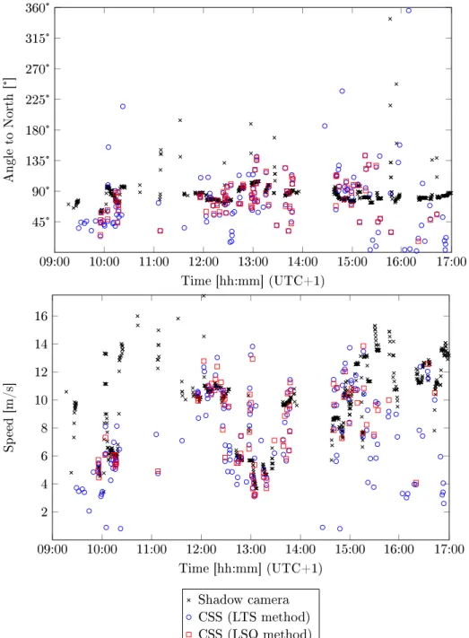
Figure 10 visualizes cloud shadow speeds on 2016-03-19 as measured by the
267
shadow camera and calculated by the two algorithmic approaches derived from
268
CSS measurements.
269
There is one dominant cloud direction (from west to east) throughout the
270
day, both for the shadow camera and the CSS. However, there is variation in
271
cloud speed due to clouds at dierent heights, as suggested by ceilometer and
272
all-sky imager data (not shown). In general, there is much scatter and large
273
deviations between the measurements. This is partially caused by multiple cloud
274
layers present on this day, which pose a challenge both for the shadow camera
275
diuse edges often do not trigger CSS measurements or only measurements with
277
low accuracy. The detection rates of the CSS for 12 shading classes are discussed
278
in section 4.4.
279
Optically thin clouds are found to be less critical for the shadow camera
280
system. Mixed situations with both optically thin and thick clouds present pose
281
a challenge for the shadow camera system. However, such mixed situations are
282
not predominant on the area imaged by the shadow camera.
283
Between 14:00 h and 14:30 h, a thick cloud is blocking the sun in the whole
284
area image by the shadow camera. The shadow camera is not able to derive
285
measurements out of this very dark shadow.
286
Applying the methodology described in section 4.2, the deviations found on
287
this day for the LSQ and the LTS method are displayed in Tab. 2.
Table 2: Deviations found for the LSQ and LTS approach in comparison to the shadow camera on 2016-03-19. Instantaneous CSS measurements without any temporal averaging are compared to±2 min medians derived from the shadow camera.
LSQ approach LTS approach RMSD 2.7 m/s,31.4° 3.9 m/s,39.5°
MAD 1.8 m/s,23.1° 2.7 m/s,29.9°
bias -0.7 m/s,8.3° -1.6 m/s,9.5° 288
09:00 10:00 11:00 12:00 13:00 14:00 15:00 16:00 17:00 45° 90° 135° 180° 225° 270° 315° 360° Time [hh:mm] (UTC+1) Angle to North [°] 09:00 10:00 11:00 12:00 13:00 14:00 15:00 16:00 17:00 2 4 6 8 10 12 14 16 Time [hh:mm] (UTC+1) Sp eed [m/s] Shadow camera CSS (LTS method) CSS (LSQ method)
Figure 10: CSS and shadow camera measurements on 2016-03-19. Due to multiple cloud layers and optically thin clouds, both scatter and signicant deviations between the CSS measurements and the shadow camera reference systems are present.
The cloud speeds and direction of 2016-04-22 are depicted in Fig. 11. On
289
this day, mainly altocumulus clouds with an altitude of 2000 m are present.
290
Both the measured cloud directions and the measured cloud speeds are not
291
homogeneous throughout the day. Between 11:00 h (UTC+1) and 12:30 h, the
292
CSS measurements scatter strongly in comparison to the reference system. Also,
293
a bias in the velocities is found. The origins of these deviations lay in a key
294
assumption of the linear cloud edge - curve tting method, which is discussed in
295
appendix A. Between 13:00 h (UTC+1) and 15:00 h, there is a high correlation
296
between the measurements.
297
Between 16:00 h (UTC+1) and 16:30 h, the CSS is shaded by clouds, but
298
does not provide any measurements. Looking at all-sky and shadow camera
299
images as well as ceilometer data reveals that this is caused by optically thin
300
clouds with diuse edges at approximately 4000 m altitude. Their speed is
301
beyond the limits of the reference system (17.5 m/s).
302
After 16:30 h (UTC+1), there is a signicant amount of scatter. All-sky
303
imager data testify multiple cloud layers during this time. The deviation found
304
on this day for the LSQ and the LTS method are displayed in Tab. 3.
Table 3: Deviations found for the LSQ and LTS approach in comparison to the shadow camera on 2016-04-22. Instantaneous CSS measurements without any temporal averaging are compared to±2 min medians derived from the shadow camera.
LSQ approach LTS approach RMSD 1.6 m/s,24.9° 1.9 m/s,37.8°
MAD 1.2 m/s,20.1° 1.4 m/s,25.6°
bias -0.8 m/s,3.9° -0.8 m/s,1.3° 305
11:00 12:00 13:00 14:00 15:00 16:00 17:00 18:00 19:00 45° 90° 135° 180° 225° 270° 315° 360° Time [hh:mm] (UTC+1) Angle to North [°] 11:00 12:00 13:00 14:00 15:00 16:00 17:00 18:00 19:00 2 4 6 8 10 12 14 16 Time [hh:mm] (UTC+1) Sp eed [m/s] Shadow camera CSS (LTS method) CSS (LSQ method)
Figure 11: CSS and shadow camera measurements on 2016-04-22. Both the cloud directions and the cloud speeds change multiple times during the day.
4.2. Comparing cloud shadow speeds: CSS against shadow camera
306
During the comparison period of 59 days, the CSS obtained 3170 cloud
307
motions vectors with the LSQ approach (for details see section 2.2). The shadow
308
camera measured 23155 cloud motion vectors. This discrepancy between the
309
amount of CSS measurements and the shadow camera approach is partially
310
caused by optically thin clouds, which often do not trigger a CSS measurement
311
(see section 4.4), and by the area of the measurements. The CSS is statistically
312
not shaded as often as the area imaged by the reference system because these
313
two areas have far dierent sizes (CSS: approximately 0.09 m2; shadow camera:
314
approximately 0.28 km2).
315
The deviations found for the LSQ method in comparison to the shadow
316
camera measurements are displayed in Tab. 4 without any temporal averaging,
317
±2 min medians (LSQ±2 min) and±5 min temporal medians (LSQ±5 min).
318
The deviations are visualized in a scatter density plot in Fig. 12. The
de-319
viations stem mostly from optically thin clouds and clouds at large altitudes
320
(see Kuhn et al. (2018b)). If such clouds trigger CSS measurements at all, the
321
accuracy is poor.
322
Table 4: Deviations found for the LSQ approach for measurements with and without temporal averaging in comparison to the shadow camera measurements on 59 days (shadow speed).
LSQ approach
LSQ
±2 minLSQ
±5 minRMSD 2.7 m/s (36.6 %) 2.4 m/s (32.7 %) 2.1 m/s (28.0 %)
MAD
1.6 m/s (21.9 %) 1.3 m/s (18.0 %) 1.2 m/s (15.7 %)
bias
-0.2 m/s (2.7 %)
-0.2 m/s (2.5 %)
-0.2 m/s (2.8 %)
(a) (b)
Figure 12: Scatter density plots of the speeds measured by the CSS and the shadow camera. Figure 12a: LSQ method without temporal averaging, Fig. 12b: LSQ method with±5 min
temporal medians. The colorbar represents the relative frequency of a given pixel within the corresponding shadow camera speed bin. Each column adds up to 100 %. In total, the LSQ method obtained 3170 measurements of which 2956 could be temporally matched to shadow camera measurements.
4.3. Comparing cloud shadow directions: CSS against shadow camera
323
This section compares the cloud shadow directions as measured by the CSS
324
against the reference shadow camera. The data set for this comparison is the
325
same as in section 4.2. The deviations found for the LSQ method in
compar-326
ison to the shadow camera regarding the shadow directions are displayed in
327
Tab. 5. Although there is only a minor bias present, the deviations do not
328
shrink signicantly with larger temporal medians. This is an indication that
329
systematic osets are present between the CSS and the shadow camera
mea-330
surements. These osets can be explained by the dierent area from which these
331
two systems derive their cloud motion vectors. For the shadow camera, this is
332
a relatively large area. Therefore, the obtained cloud motion direction is an
333
average direction. The CSS, however, might be able to resolve smaller cloud
334
movements, e.g. rotations or very small clouds (such as the clouds at 12:15 h,
335
2016-10-14, as discussed in section 4.1). Furthermore, the CSS measurements
336
are based on the assumptions of the linear cloud edge - curve tting method,
Table 5: Deviations found for the LSQ approach in comparison to the shadow camera approach on 59 days with and without temporal averaging (shadow motion direction,180°=100 %).
LSQ approach LSQ
±2 minLSQ
±5 minRMSD
50
.
2
° (28.0 %)
52
.
2
° (29.0 %)
47
.
9
° (26.6 %)
MAD
30
.
4
° (16,8 %)
28
.
2
° (15.6 %)
25
.
3
° (14.0 %)
bias
0
.
5
° (0.2 %)
3
.
4
° (2.0 %)
3
.
7
° (2.0 %)
which is visualized in Fig. 2 and discussed in appendix A. If e.g. a cloud shades
338
the CSS with a saw tooth edge of suitable size, the measured direction might
339
not be the general direction of the cloud. Such systematic osets could explain
340
the behavior seen in Tab. 5 as well as the scatter seen in Fig. 13.
341
(a) (b)
Figure 13: Scatter density plot of CSS LSQ without temporal averaging (a) and CSS LSQ with
±5 min temporal medians (b) cloud directions versus the shadow camera cloud directions.
The colorbar represents the relative frequency of a given pixel within the corresponding shadow camera direction bin.
4.4. Investigating the detection rate of the CSS
342
In section 2.2, a method to increase the detection rate of the CSS is discussed.
343
The validation presented in this section is conducted on 223 days (from
2016-344
comparison to the shadow camera, but in comparison to normalized irradiance
346
measurements of the CSS itself. This approach is chosen to avoid scale eects
347
between the shadow camera and the CSS. These scale eects are clouds seen by
348
the CSS but not by the shadow camera, clouds imaged by the shadow camera
349
but not shading the CSS and shadows beyond the temporal resolution of one
350
system. The approach to investigate the detection rate of the CSS by looking
351
at the CSS raw data is described in the following.
352
Figure 14 displays an example day as measured by one of the nine CSS sen-sors. A clear sky global horizontal irradiance (CSF) model described in Han-rieder et al. (2016) is added and the sensor signals are calibrated to the mea-surements of a close-by GHI reference station. Furthermore, the 9 s missing data after each 9 s measurement are linearly interpolated. Using a clear sky
09:00 10:00 11:00 12:00 13:00 14:00 15:00 16:00 17:00 100 200 300 400 500 600 700 800 900 Time [hh:mm] (UTC+1) Sensor signal [W/m 2 ]
Figure 14: Example day with added clear sky reference (2016-08-25). DHI overshootings and shading events caused by transient clouds are visible.
modeling (CSM), shading strengths (SS) can be dened (Mäki and Valkealahti, 2012):
SS= GHI
CSM−GHI
GHICSM (10)
In equation 10, GHI is the measured and calibrated irradiance from one of the
353
9 CSS sensors andGHICSM is the modeled clear sky irradiance. Calibration is
354
performed using another calibrated reference pyranometer approximately 500 m
away from the CSS and a dynamic adaption factor for the CSS sensor signal.
356
The deviations from the modeled clear sky irradiance are used to determine the
357
amount of shading events detected by the CSS. A shading event begins after
358
the ratio of the measured GHI and the clear sky GHI falls below 90 % and ends
359
if it is again above this threshold. The shading strength is derived from the
360
minimum measured GHI between these two timestamps.
361
All shadings are characterized into 12 classes by their shadings strengths and
362
shading duration. Shading strengths are divided into three dierent classes:
363
≤30 % for optically thinner clouds
364
> 30 % and≤60 % for thicker thin clouds
365
> 60 % for optically thicker clouds
366
Shading durations are resolved into four classes:
367
≤60 s for short shading durations
368
> 60 s and≤300 s for medium shading durations
369
> 300 s and≤600 s for long shading durations
370
> 600 s for (partial) overcast situations
371
The relative share of each class as measured from 2016-03-20 to 2016-10-28
372
(223 days) is shown in Tab. 6. Predominantly, there are optically thin clouds
373
with short shading durations above the PSA.
Table 6: Classications based on shading strength and shading duration: Amount of events per class from 2016-03-20 to 2016-10-28 (223 days). Optically thin clouds with short shading durations are most common. Total amount of shading events (per sensor): 8276.
Shading duration [s] < 60 60 300 300 600 > 600 sum Shading strengh > 60 % 3.4 % 3.8 % 0.9 % 2.4 % 10.5 % 30 60 % 18.3 % 8.4 % 1.8 % 1.9 % 30.4 % < 30 % 52.9 % 5.3 % 0.7 % 0.3 % 59.1 % sum 74.6 % 17.4 % 3.4 % 4.6 %
In Tab. 7, the detected CSS measurements per shading class are depicted
375
using the LSQ approach. The CSS measures only 4.8 % of optically thin clouds
376
with shading durations above 600 s and is best for optically thick clouds with
377
short shading durations (21.6 % detected events). The rate of successfully
de-378
tected shading events is low.
379
Using the LSQ approach (see section 2.2) 5830 shading events are detected
380
between 2016-03-20 and 2016-10-28 ( 223 days).
381
Table 7: Detection rates for each shading class: Relative share of shading events detected by the CSS using the LSQ algorithm from 2016-03-20 to 2016-10-28 (223 days). Total amount of detected shading events: 8276.
Shading duration [s] < 60 60 300 300 600 > 600 Shading strength > 60 % 21.6 % 16.4 % 16.7 % 9.5 % 30 60 % 16.0 % 13.7 % 9.5 % 6.3 % < 30 % 8.0 % 3.7 % 3.7 % 4.8 %
4.5. Comparing CSS software approaches: LSQ and LTS
382
In section 2.2, the methodology used by the CSS to derive cloud motion
383
vectors is presented and ways to increase the dectection rate are discussed. As
384
can be seen in section 4.4, the detection rate is low. This can be improved
385
by using the LTS approach instead of the LSQ approach. In this section, the
386
deviations found in comparison to the shadow camera using the CSS with the
387
LTS approach are investigated. Moreover, these deviations are compared to the
388
deviations obtained with the CSS and the LSQ approach.
389
In comparison to the histogram found for the LSQ approach (see Fig. 7), no
390
signicant deviations are present. During the comparison period of 59 days, the
391
CSS obtained 6041 cloud motion vectors using the LTS method (3170 for the
392
LSQ approach, 23155 with the shadow camera).
393
The deviations found for the LSQ and LTS method in comparison to the
394
shadow camera measurements are displayed in Tab. 8 without any temporal
395
averaging, ±2 min medians and±5 min medians. The LTS approach shows
396
higher deviations in comparison to the shadow camera. However, for±5 min
397
temporal medians (LSQ: 2705 temporally averaged measurements with
corre-398
sponding shadow camera reference measurements, LTS: 4350 measurements),
399
the deviations for both LSQ and LTS are similar.
400
In general, the measurements obtained by the LTS method are less accurate,
401
but far more frequent in comparison to the LSQ method. This is also visualized
402
in the scatter density plots in Fig. 15.
403
Table 9 investigates the origin of the larger deviations found using the LTS
404
method. LTS∈LSQ derives the deviations for all LTS measurements which are
405
Table 8: Deviations found for the LSQ and LTS approach for measurements with and without temporal averaging in comparison to the shadow camera measurements on 59 days (shadow speed).
LSQ approach LSQ±2 min LSQ±5 min LTS approach LTS±2 min LTS±5 min RMSD 2.7 m/s (36.6 %) 2.4 m/s (32.7 %) 2.1 m/s (28.0 %) 3.4 m/s (45.8 %) 2.9 m/s (39.2 %) 2.6 m/s (35.2 %) MAD 1.6 m/s (21.9 %) 1.3 m/s (18.0 %) 1.2 m/s (15.7 %) 2.1 m/s (28.0 %) 1.7 m/s (22.4 %) 1.5 m/s (20.2 %) bias -0.2 m/s (-2.7 %) -0.2 m/s (-2.5 %) -0.2 m/s (-2.8 %) -0.4 m/s (-5.8 %) -0.4 m/s (-5.1 %) -0.4 m/s (-5.7 %)
Table 9: Deviations found for LTS approach adjacent and not adjacent to obtained LSQ measurements in comparison to the shadow camera measurements on 59 days (shadow speed).
LTS∈LSQ LTS∈LSQ±1 min LTS6∈LSQ LTS6∈LSQ±1 min
RMSD 2.9 m/s (39.0 %) 2.4 m/s (32.0 %) 5.4 m/s (73.2 %) 5.2 m/s (70.6 %) MAD 1.8 m/s (24.2 %) 1.4 m/s (19.3 %) 3.7 m/s (49.7 %) 3.5 m/s (47.2 %) bias -0.2 m/s (-3.0 %) -0.2 m/s (-2.7 %) -1.6 m/s (-21.2 %) -1.6 m/s (-21.8 %) within±1 min around a LSQ measurement (3517, 84.8 %). LTS∈LSQ2 min
406
compares these±1 min temporal medians to the shadow camera measurements.
407
LTS 6∈ LSQ calculates the deviations for LTS measurements, which are not
408
within ± 1 min around a LSQ measurement (630, 15.2 %). LTS6∈LSQ2 min
409
derives the deviations for these measurements as medians over±1 min.
410
The measurements rejected by the LSQ approach but accepted by the LTS
411
method show far higher deviations in comparison to the shadow camera
mea-412
surements. Thus the LTS method, providing more measurements, shows similar
413
deviations for situations in which the LSQ method obtains measurements but
414
displays high deviations otherwise.
415
Figure 15b compares the velocities derived from the LSQ and LTS method
416
to each other by taking the±2 min median of the LSQ measurements around a
417
LTS measurement. No systematic bias is present and there is a high correlation.
418
The largest deviations occur for velocities above 15 m/s.
(a) (b)
Figure 15: Scatter density plots of measured cloud speeds on 59 days. Figure 15a: LTS method (no temporal averaging, compare to Fig. 12), Fig. 15b: LSQ-LTS comparison. The colorbar represents the relative frequency of a given pixel within the corresponding shadow camera speed bin. Each column adds up to 100 %. In total, with the LSQ and LTS method, 3170 and 6041 measurements could be obtained, respectively. The shadow camera produced 23155 measurements.
The deviations found for the LSQ and LTS method in comparison to the
420
shadow camera regarding the shadow directions are displayed in Tab. 4.5.
Simi-421
lar to the deviations found for the velocities, the deviations for the LTS method
422
are larger. However, more measurements are obtained with the LTS method
423
in comparison to the LSQ method. As discussed for the direction deviations
424
derived with the LSQ method (see section 4.3), temporal averaging does not
425
reduce deviations as strongly as for the cloud velocities (compare with Tab. 8).
426 427
Table 10: Deviations found for the LSQ and LTS approach in comparison to the shadow camera approach on 59 days with and without temporal averaging (shadow motion direction, 180°=100 %).
LSQ approach LSQ±2 min LSQ±5 min LTS approach LTS±2 min LTS±5 min
RMSD 50.2° (28.0 %) 52.2° (29.0 %) 47.9° (26.6 %) 58.4° (32.4 %) 56.0° (30.8 %) 55.2° (30.6 %)
MAD 30.4° (16,8 %) 28.2° (15.6 %) 25.3° (14.0 %) 35.7° (20.0 %) 30.8° (17.2 %) 30.0° (16.4 %)
In Fig. 16, the LTS derived cloud shadow directions without temporal
aver-428
aging are compared to corresponding shadow camera measurements and
mea-429
surements obtained from the CSS-LSQ approach. Although the measurements
430
align, there is a signicant amount of scatter.
431
(a) (b)
Figure 16: Scatter density plot of CSS LTS cloud directions without temporal medians versus the shadow camera cloud directions (a) and versus CSS LSQ cloud directions (b), both with temporal medians of±2 min.
Figure 16b compares the directions obtained from the CSS with the LSQ
432
and LTS method using a scatter density plot. The approach is similar to the
433
approach for Fig. 15b. Although there is scatter, the two methods provide
434
similar cloud directions for temporally adjacent measurements (see Tab. 9).
435
As a conclusion, the LTS method obtains more measurements than the LSQ
436
method. However, for LTS measurements not temporally adjacent to LSQ
mea-437
surements, the deviations in comparison to the shadow camera are large.
How-438
ever, for some applications (e.g. industrially used cloud height measurement
439
systems) a less accurate measurement might be better than no measurement at
440
all and the LTS method can provide this trade-o.
5. Caveats, advantages and disadvantages of the CSS and the novel
442
shadow camera approach
443
The shadow camera needs proper orientation, an elevated position and an
444
area with little non-cloud movements. Also, pixels imaging mirrors and other
445
reective objects cannot be evaluated. Furthermore, evaluating pixels imaging
446
photovoltaic panels or larger vegetation (e.g. forests) is dicult. Although the
447
lack of a strongly elevated position can be overcome by using elevated structures
448
of lower height (e.g. 10 m) and a higher image acquisition frequency, such a
449
system would have a disadvantage due to the smaller imaged area. If needed,
450
this issue could be overcome using multiple cameras.
451
One major disadvantage of this particular shadow camera is the temporal
452
availability of historic images. If an image is taken only every 15 s, very fast
453
clouds will already have transitioned past the image area. Changing the
tempo-454
ral resolution to multiple images per second requires only a simple software
ad-455
justment in the camera, but the data storage requirements become prohibitive.
456
For instance, a camera taking 3 MP images every 15 s accumulates on one day
457
over 12 h approximately 0.7 GB of data (255.5 GB per year). An image
ac-458
quisition rate of 1 s would increase this gure to approximately 10.4 GB per
459
day (3.8 TB per year). If 25 images are taken every second, one 3 MP camera
460
produces approximately 259 GB of data during 12 h (94.5 TB per year).
461
If only real-time cloud shadow speeds are of interest, the maximum
tem-462
poral resolution is just limited by the calculation time. The required time to
463
derive cloud motion vectors strongly depends on the data transmission rate
464
and can in total be below 1 s, which is faster than the calculations of the CSS.
465
With higher temporal resolutions, the area needed to derive (fast) cloud shadow
466
speeds shrinks. However, as many cloud motion vectors should be measured, the
467
imaged area should not be below a certain minimum. This minimum depends
468
on local characteristics and restrictions as well as the intended application.
469
The CSS however is a fairly compact device, which can be installed at every
470
position which is not shaded by objects. A disadvantage is the detection rate
and detection accuracy regarding optically thin clouds. As these clouds are less
472
relevant for e.g. photovoltaic nowcasting applications, this might be acceptable.
473
In direct comparison, the shadow camera obtains more measurements, which
474
scatter less. Also, optically thin clouds can be measured more accurately than
475
with the CSS. Furthermore, the shadow-camera-based approach takes the
av-476
erage cloud motion vector over a larger area, which is more likely to contain
477
cloud shadows than the relatively small area covered by the CSS. Moreover,
478
due to the nite size of cloud shadows, the shadow camera does not face the
479
challenge of the linear cloud edge - curve tting method as strongly as the CSS
480
(see section A).
481
In general, both systems require little to no maintenance and were found to
482
be robust in the harsh environments present in the desert of Tabernas.
Specif-483
ically, the downward-facing shadow cameras require far less maintenance than
484
the upward-facing all-sky imagers.
485
6. Conclusion and future work
486
On 59 days, the cloud shadow speeds and the cloud directions measured by
487
the CSS are compared to a novel shadow camera approach for two algorithmic
488
methods. For±5 min temporal medians, deviations of RMSD 2.1 m/s (28.0 %),
489
MAD 1.2 m/s (15.7 %) and a bias of -0.2 m/s (2.8 %) are found. Deviations of
490
the cloud shadow direction are RMSD47.9° (26.6 %), MAD25.3° (14.0 %) and 491
a bias 3.7° (2.0 %). An alternative algorithm, obtaining more measurements, 492
shows higher deviations. In addition to that, the detection rate of the CSS is
493
determined to be between 3.7 % and 21.6 % depending on the shading class on
494
223 days.
495
The eects of the linear cloud edge - curve tting method are studied and
496
potential solutions discussed. The eects were found to be of minor importance.
497
Potential corrections approaches were found to increase deviations. Thus, we
498
suggest not applying them.
499
As the CSS and the reference shadow camera can be used for the same
purposes, the specic advantages and disadvantages are discussed. The CSS
501
is found to be the more exible tool. However, given certain infrastructural /
502
geographical requirements, the shadow camera might be the better choice. Both
503
systems do not require regular maintenance and come with a small price tag
504
(although the CSS is currently not commercially available).
505
As shown, strict ltering of CSS measurements leads to very little data with
506
many shading events not being measured. If the ltering is less strict, the
mea-507
surements show larger deviations. Depending on the application, a less accurate
508
measurement might be more desirable than no measurement at all. For instance,
509
if clouds speeds are used to obtain cloud heights for a nowcasting system used
510
in industry, less accurate measurements can be preferable to missing
measure-511
ments. If on the other hand reference data for validations are to be obtained,
512
accuracy might be more important than the total amount of measurements.
513
Therefore, as a software improvement, we suggest making this decision based
514
on the requirements for each application.
515
The CSS used in this study measures for 9 s and stores the results afterwards,
516
which causes a dead time of another 9 s. Although this dead time can be
517
interpolated, continuous measurements would further improve the device. In
518
a redesigned version of the CSS (developed in late 2016), the dead time was
519
reduced to 2 s. Future hardware improvements should further reduce this dead
520
time.
521
In many cases, cloud shadow speeds are not the nal measurement of interest
522
but only an intermediate result. Depending on the intended application of
523
the CSS, several other potential hardware adaptions could be implemented.
524
If irradiance values are of interest, one or several sensors of the CSS could
525
be calibrated and thus used to measure GHI. Integrating a rotating shadow
526
band (RSI) into the CSS would further enable direct normal irradiance (DNI)
527
measurements. If the CSS is used as a part of an all-sky imager based nowcasting
528
system or utilized to derive cloud heights, an inexpensive camera could be added,
529
providing a complete system. A CSS and a shadow camera based system, which
530
same 59 days in another publication (Kuhn et al., 2018b).
532
In the near future, site evaluations for photovoltaic plants might include
533
mean and maximum cloud speeds as these values impact the size of buers
534
needed to fulll ramp rate regulations. The easy-to-deploy CSS can be used to
535
obtain this information.
536
With additional hardware added, the CSS can be upgraded to be a solar
537
nowcasting system in a box, providing irradiance predictions for solar power
538
plants. As currently ramp rate regulations for photovoltaic plants are discussed,
539
which can be fullled with the help of nowcasting systems, such systems may
540
support the integration of large solar penetrations into our electricity grids.
541
Acknowledgements
542
The research presented in this publication has received funding from the
Eu-543
ropean Union's Horizon 2020 program for the initial development of the shadow
544
camera system (PreFlexMS, Grant Agreement no. 654984). With founding
545
from the German Federal Ministry for Economic Aairs and Energy within
546
the WobaS project, the shadow camera system was developed. The European
547
Union's FP7 program under Grant Agreement no. 608623 (DNICast project)
548
nanced operations of the all-sky imagers and other ground measurements. The
549
authors are also grateful for the nancial support provided by project PRESOL
550
with reference ENE2014-59454-C3-2-R, funded by the Ministerio de Economía y
551
Competitividad and co-nanced by the European Regional Development Fund
552
(FEDER). Thanks to the reviewers for their helpful comments and to our
col-553
leagues from the Solar Concentrating Systems Unit of CIEMAT for the support
554
provided in the installation and maintenance of the shadow cameras. These
555
instruments are installed on CIEMAT's CESA-I tower of the Plataforma Solar
556
de Almería.
Appendix A Angle correction and the linear cloud edge - curve
558
tting method
559
Here, basic assumptions of the linear cloud edge - curve tting method are
560
studied and potential solutions discussed. The considerations are not only
rele-561
vant for the CSS, but for many other velocity deriving systems. These
investiga-562
tions require a reference system. The shadow camera provides such references,
563
enabling us to carry out these studies on the CSS. To the best of our
knowl-564
edge, this is the rst time such an in-eld investigation of the aperture problem
565
is performed.
566
A.1 The aperture problem on one example day
567
The aperture problem is a very fundamental challenge for many velocity
de-568
riving systems. Several publications on the CSS and on similar systems (Bosch
569
and Kleissl (2013), Bosch et al. (2013), Lappalainen and Valkealahti (2016a),
570
Lappalainen and Valkealahti (2016b)) use the linear cloud edge method to
over-571
come this problem. In this method, the cloud speed and the moving direction
572
of the cloud are determined from the measurements obtained by two shading
573
anks with assumed identical cloud motion vectors. To avoid this assumption,
574
the "linear cloud edge - curve tting method" is implemented in the CSS (Wang
575
et al., 2016). This method assumes that the motion of a cloud is always
per-576
pendicular to the cloud edge (see Fig. 1). If the cloud edge is not perpendicular
577
to the moving direction of the cloud, the cloud speed is underestimated by the
578
factorcosδ, whereδrepresents the angle between the speed vector and the
nor-579
mal of the shadow edge. This question has been addressed in previous works
580
but no sucient answer has been found yet (Bosch et al. (2013), Lappalainen
581
and Valkealahti (2016a)). With the shadow camera acting as a reference, the
582
eects of these systematic deviations can be studied and reversed. Figure A.1
583
visualizes the raw data of the CSS measurements and the shadow camera
mea-584
surements for speed and direction for one example day (2016-04-25) without
585
any temporal averaging for both systems. The CSS measurements scatter in a
09:00 10:00 11:00 12:00 13:00 45° 90° 135° 180° 225° 270° 315° 360° Time [hh:mm] (UTC+1) Angle to North [°] 09:00 10:00 11:00 12:00 13:00 1 2 3 4 5 6 7 8 9 10 Time [hh:mm] (UTC+1) Sp eed [m/s]
Cloud Speed Sensor Shadow camera corrected CSS speed
Figure A.1: CSS measurements and the raw data of the shadow camera on 2016-04-25. This example is used to illustrate the eects of the linear cloud edge method.
signicant range, whereas the shadow camera system cloud motion directions
587
show almost no scatter at all and only a minor number of outliers throughout
588
the day. The low level of scatter and bias in the raw data is a strong
indica-589
tion that the direction detected by the shadow camera is correct. We will show
0 15 30 45 60 75 90 2 4 6 8 10 12 14 16 18 20 Angular deviationδ[°] Relativ e frequency [%]
Figure A.2: Angular deviationδon 2016-04-25 between the one-shadow-camera system and
the CSS, depicted for the LSQ method. There is a total of 118 CSS measurements using the LSQ method.
in this section that scatter in the CSS data is partially caused by cloud edges
591
passing the CSS not being perpendicular to the motion vectors.
592
In the following, the moving direction measured by the shadow camera is
593
considered the true direction of the clouds, which appears justied because its
594
scatter is very small. The distribution of the thus measured angular deviation
595
δ between the CSS measurements (displayed for the LSQ method) and the
596
reference system is shown in Fig. A.2. The deviations are signicant and result
597
in systematically too small speeds as measured by the CSS.
598
Withδknown, the CSS speed can be corrected according to equ. A.1
(com-599
pare with Fig. 2). The corrected CSS velocities are depicted with + in the
600
bottom part of Fig. A.1. Due to the correction, the scatter is reduced from
601
0.9 m/s to 0.7 m/s standard deviation. Furthermore, the corrected average
602
speed (5.7 m/s) on this day of is closer to the average speed as measured by the
603
shadow camera (6.2 m/s) than the uncorrected average speed (5.1 m/s).
604
vcorr =vCSS (A.1)
A.2 Investigating potential solutions
606
Assuming that the bias (presented in section 4.5) is only caused by cosδ,
607
we can calculate the average angular oset δavg,i using the average velocities
608
derived with the LSQ and LTS method and equ. A.1, equ. A.2 and equ. A.3.
609 bias= 1 N N X i=1
(vCSS,i−vSC,i) =vavg,CSS−vavg,SC (A.2) 610
611
cosδavg,i= vavg,CSS,i
vavg,CSS,i−bias (A.3)
612
For the LSQ method with an average speed of 8.61 m/s and a bias of
-613
0.21 m/s for ±5 min medians, an δavg,LSQ = 12.4° is found (cosδavg,LSQ = 614
0.977). For the LTS method (±5 min medians) with an average speed of 8.48 m/s
615
and a bias of -0.42 m/s, an δavg,LTS = 17.8° is found (cosδavg,LTS = 0.952). 616
However, as we can see in the previous section on one example day, the bias is
617
not completely caused by δ. Therefore, this eect is arguably not of outmost
618
importance or hidden behind other deviations.
619
The correction made in the previous section and the bias correction made
620
here could only be accomplished using a reference measurement system. Several
621
approaches are possible to make such a correction without reference
measure-622
ments and will be studied in the following.
623
A.2.1 Calculate corrections factors based on cloud speeds
624
A correction approach for cosδ based on cloud speeds is discussed (Wang
625
et al., 2016, section 4.3), but could not be tested due to the lack of a reference
626
system. Using the shadow camera measurements, this suggested correction is
627
investigated in this section. The suggested approach can be made operational
628
by using the maximum velocity measured during a given period of time for all
629
corresponding measurements. The maximum velocity is thus considered to be
630
vreal. Additionally, this velocity is considered to be perpendicular to the cloud
631
edge. Both assumptions are questionable.
Table A.1: Cloud speed deviations found for the LSQ and LTS approach with speed-derived corrections applied in comparison to the shadow camera measurements on 59 days.
LSQ±2 min,corr,max LSQ±5 min,corr,max LTS±2 min,corr,max LTS±5 min,corr,max
RMSD 3.1 m/s (41.7 %) 3.7 m/s (50.8 %) 3.9 m/s (53.6 %) 4.7 m/s (64.3 %) MAD 1.8 m/s (24.0 %) 2.1 m/s (29.1 %) 2.4 m/s (32.5 %) 3.0 m/s (40.3 %) bias 1.0 m/s (+14.0 %) 1.6 m/s (+22.9 %) 1.4 m/s (+19.2 %) 2.4 m/s (+32.0 %)
Table A.1 shows the deviations found if the maximum speed measured in a
633
period of time is compared to the medians of the shadow camera for the same
634
period. In comparison to Tab. 8, in which the deviations without this correction
635
are presented, the deviations shown here are signicantly larger. Especially the
636
bias, which is now positive, is increased by this correction. The larger deviations
637
are caused by the scatter present in the CSS measurements (visualized in the
638
plots of section 4.1). Moreover, cloud speeds might change signicantly within
639
±5 min. Thus, this correction approach is not feasible.
640
A.2.2 Calculate corrections factors based on cloud directions
641
Another approach to derive correction factors for cloud speeds not
perpen-642
dicular to the corresponding cloud edges is based on the directions. For a period
643
of time, a median cloud motion direction is calculated. This way,cosδ can be
644
estimated for every measurement and the velocities can be corrected. Thus
645
derived,δ is Gaussian distribution with a standard deviation of e.g. 52.8° for 646
LSQ±2 min,corr.
647
In Tab. A.2, the deviations in comparison to the shadow camera
measure-648
ments are shown. Osets greater than one standard deviation are not corrected.
649
Including these corrections leads to higher deviations. The velocities are not
fur-650
ther temporally averaged within the considered time periods.
651
In comparison to Tab. 8, Tab. A.2 shows higher deviations. Increasing the
652
period of time to calculate the median cloud motion vectors from ±2 min to
653
±5 min increases the RMSD and MAD. Notably, the bias is reduced. In
sum-654
mary, we conclude that this correction approach is not feasible. The reason for