Audio Object Separation Using Microphone Array Beamforming

Audio object separation using microphone array beamforming

Philip Coleman

, Philip J. B. Jackson

, and Jon Francombe

Centre for Vision, Speech and Signal Processing, University of Surrey, Guildford, Surrey, GU2

7XH, UK

2

Institute of Sound Recording, University of Surrey, Guildford, Surrey, GU2 7XH, UK

May 2015

Abstract

Audio production is moving towards an object-based ap-proach, where content is represented as audio together with metadata that describe the sound scene. From cur-rent object definitions, it would usually be expected that the audio portion of the object is free from interfering sources. This poses a potential problem for object-based capture, where microphones cannot be placed close to a source. In this paper, the application of microphone array beamforming is investigated for its ability to sep-arate a mixture into distinct audio objects. Real mix-tures recorded by a 48 channel microphone array in re-flective rooms were separated, and the results were evalu-ated using perceptual models in addition to physical mea-sures based on the beam pattern. The effect of interfering objects was reduced by applying the beamforming tech-niques.

1

INTRODUCTION

Object-based audio gives advantages over the traditional channel-based approach in terms of creative control, scal-ability across various rendering systems, and interactivity with audio content [1]. A sound scene would ideally be captured in such a way that it could be represented arbi-trarily in space (as desired by the producer), and transmit-ted without knowledge of the reproduction system (which would decode the scene in the way most appropriate to the

context). This is referred to as a format-agnostic system. There are currently two main approaches for recording multiple active sources for audio production: close cap-ture and spatial capcap-ture. Close capcap-ture aims to maximise the signal-to-noise ratio (SNR) of the source by placing a microphone as close to it as possible. In addition to achieving a high SNR (which is beneficial for separation from other sources and in terms of reducing the effects im-posed by the recording space itself), close capture record-ings can very easily be converted into conventional audio objects with the addition of metadata describing the posi-tion. However, they contain no inherent spatial informa-tion. Spatial microphone techniques, which use multiple microphone capsules and therefore contain some spatial information about the scene (including the performance and the room), are therefore often used. Examples of spa-tial microphone techniques include stereo or multichannel arrangements (which correspond directly to loudspeaker channels) [2], binaural recording using a dummy head, room ambience capture (e.g. a Hamasaki square [3]), and using a soundfield microphone which gives 3-D informa-tion encoded on to orthogonal basis funcinforma-tions (usually B-format). However, these techniques carry two main dis-advantages. First, the audio for individual sound sources is not available. Second, each technique (with the excep-tion of the soundfield microphone) is directly related to a specific channel-based reproduction system, limiting the general application of such techniques. In principle, the spatial information from the soundfield microphone can

be recovered and processed, although there is an inherent physical limitation given the small spatial extent of the microphone.

A dense microphone array [4] has the potential to cap-ture a sound scene in a format-agnostic manner. The microphone array receives spatial information about the scene, and gives the opportunity to apply spatial filtering or other signal processing (e.g. to improve the SNR) by having a relatively large number of capsules with dense spacing. The concept of spatial filtering, or beamforming, is well established. The purpose of a beamformer is to estimate the signal arriving from a certain direction, usu-ally in the presence of noise and interference [5]. Beam-forming algorithms applied to microphone arrays can be categorized into three approaches: additive (the signals are filtered and summed to achieve the output); differen-tial (the microphones are closely spaced and so the ar-ray is sensitive to the derivative of the sound pressure); and eigenbeamforming (based on decomposing the sound field onto orthogonal basis functions) [6]. Additionally, optimal beamformers such as the minimum variance dis-tortionless response (MVDR) can be formulated in the spherical harmonics domain [7]. For audio capture, a cylindrical harmonic description has previously been used to create coincident directive virtual microphones [8]. In this paper, additive beamformers are used as they are gen-erally applicable without requiring specific array geome-tries.

The beamforming methods introduced above do not en-compass the full range of techniques that can be applied to a microphone array for object separation. Blind source separation (BSS) techniques can be applied to a micro-phone array, and the additional spatial resolution gained with a microphone array has been considered explicitly by defining a space-time-frequency transform [9]. This pro-cessing has potential for a sparse representation of the re-ceived signals at the array, being able to separate sources that are active in the same time-frequency bin but are spa-tially separated.

In addition, the microphone array signals may be used to estimate some of the object metadata, including cur-rently standardised parameters (e.g. source position) and other potentially useful information (e.g. parameterized room acoustics [10]). In particular, the microphone array can be used to determine the direction of arrival (DOA) of the sources. If a microphone array is positioned in a

recording session with the perspective of a listener (simi-lar to recording with a stereo microphone pair or binaural dummy head), then knowledge of the DOA could be ad-equate to suggest prototype metadata for the content pro-ducer (or, in principle, to fully automate source position-ing). Otherwise, multiple microphone arrays with known geometry could be used to fully determine the source po-sition. Methods for determining the DOA can be broadly catergorized into time-delay estimation (e.g. [11]), spatial spectral estimation (e.g. [12]), and sound field analysis (e.g. [13]). In this paper it is assumed that the DOA is known.

Some recent work has considered the issue of format-agnostic audio capture. Audio objects derived directly from multiple microphone signals have previously been captured using a number of shotgun microphones, sound-field microphones, and an Eigenmike, and applied to a football match [14]. In particular, the Eigenmike was used for ambient sounds, and twelve shotgun microphones placed around the pitch were used to detect ball kicks and the referee’s whistle blows. Salient audio was identified from the shotgun microphone feeds, and where a single event was detected on multiple microphones the geomet-rical information was further used to localise the event to a position on the pitch. Capture of format-agnostic audio has also been considered in relation to MPEG-H [15, 16]. In this case, most objects were derived from clean mono and stereo microphone feeds, and an eight-cardioid 3-D array was used to capture the ambience. The authors com-ment that the 3-D array provided an increased sense of immersion, but they experienced some issues with spill on the ambience recordings. Application of spatial filtering and source separation techniques may therefore enhance the approach taken.

This paper is structured as follows. In Sec. 2, spa-tial filtering techniques for audio object separation are introduced, and in Sec. 3 metrics for evaluation of ob-ject separation are described. Two experiments, whereby speech and music data were recorded in real-world reflec-tive acoustic environments, are described in Sec. 4. In Sec. 5 results obtained by applying beamforming algo-rithms to the speech and music signals are presented. Fi-nally, the outlook of the work is discussed in Sec. 6 and the work is summarized in Sec. 7.

2

SPATIAL FILTERING

A number of classical beamformers are very well es-tablished and still useful in modern applications. In particular, the delay and sum (DS) and MVDR beam-formers, included in a 1988 review article [5], are still widely used [17, 18, 19]. These algorithms also repre-sent the data-independent (DS) and statistically optimum (MVDR) approaches to beamforming. Data-independent beamformers are based purely on the microphone array geometry (and in some cases the room response, if cal-ibrated in a real room), whereas statistically optimum beamformers exploit the signals received at the micro-phones. In the following the DS and MVDR beamformers are introduced, together two further methods: the superdi-rective array (SDA), a high resolution data-independent beamformer; and the linearly constrained minimum vari-ance (LCMV) beamformer, which is a generalization of MVDR.

2.1

Signal model

Consider an array ofM microphones. The signalx_m(n)

received at the mth sensor may be transformed into the frequency domain via discrete-time Fourier trans-form and written as X_m(ω), belonging to a vector of lengthM,x(ω) = [X1(ω),X2(ω), . . . ,XM(ω)]

T_{. A}

com-plex filter weight w_m(ω) can be applied at each

mi-crophone to perform spatial filtering, with w(ω) =

[w₁(ω),w₂(ω), . . . ,w_M(ω)]T, and the output of the beam-former can be written as

Y(ω) =wH(ω)x(ω), (1) with frequency dependence omitted for clarity in the fol-lowing. It is often useful to explicitly considerxas com-prising signal and (uncorrelated) noise components, such that

x=as+n, (2)

whereais the array manifold vector describing the acous-tic paths (transfer function) between the sourcesand each microphone, andndescribes the uncorrelated background noise at each microphone. The array manifold vectorain principle incorporates room reflections, although beam-formers are often calculated based on the assumption of free-field conditions.

2.2

Beamforming algorithms

In the following sections the DS, SDA, MVDR, and LCMV beamformers are formally introduced. In this pa-per the beams are steered in azimuth only, although the methods readily extend to three dimensions. Furthermore, the sources are assumed to be static, with their positions knowna priori.

2.2.1 Delay and sum beamformer

The DS beamformer exploits the known array geometry to align the received signals such that they constructively interfere towards the target direction. The output signal is conventionally written in the time domain as

y(n,θ_t) = M

∑

x_m(n−∆_m(θ_t)), (3)

wherey(n)is the inverse Fourier transform ofY(ω), and ∆mis a delay calculated based on look directionθt (from

which the desired sound will impinge on the array). Nar-rowband filter weights w(θt)can equivalently be

calcu-lated in the frequency domain as a frequency-dependent phase shift.

2.2.2 Superdirective array

The superdirective array (SDA) minimizes the isotropic acoustical noise at all directions other than the target, and can include a diagonal loading term to regularize the so-lution magnitude. In this case, the SDA weights for each frequency are calculated by [20]

w(θt) = (R_vv+εI)−1a(θt) a(θt)H(Rvv+εI) −1_a( θt) , (4) where R_vv=1 L L

∑

whereθldenotes thelth look angle,εis a weighting

pa-rameter which (physically) trades white noise gain against directivity (see Sec. 3), andIis the identity matrix with dimensionsM×M.

2.2.3 MVDR and LCMV beamformers

The MVDR and LCMV beamformers both utilize linear constraints, and rely on an estimate of the data covari-ance matrix. The principle of the MVDR beamformer is to minimize the overall output power of the array, subject to keeping unity gain in the target direction. The opti-mization problem can be written as

min

w w H_R

xxws.t.wHa(θt) =1, (6)

whereR_xx=E[xxH]denotes the spatial correlation ma-trix, θt denotes the target angle of incidence, and E[·]is

the expectation operator.

Adding diagonal loading as for the SDA above, the so-lution to the cost function is [18]

w(θt) = (R_xx+εI)−1a(θt) a(θt)H(Rxx+εI) −1_a( θt) . (7)

The solution in Eq. 7 attempts simultaneously to perform dereverberation and noise reduction. The beamformer is very often used for noise reduction only, i.e.wHR_nw

is minimized subject to the distortionless constraint (as Eq. 6), whereR_n=E[nnH]. Further forms may make use of the estimated spatial correlation matrix of the noise-free term in Eq. 2 [21]. In practice, this means that some noise-only portions of the signal must be identified, which implies a high level of supervision. If both signal and noise components can be estimated, the MVDR becomes the max-SNR beamformer [5].

The MVDR beamformer is a special case of the lin-ear constrained minimum variance (LCMV) beamformer, which gives the opportunity to impose additional con-straints on the solution. For instance, if an interferer is known to exist at a certain location θi, the LCMV cost

function can be formulated as [18] min w w H_R xxws.t.w H_a( θt) =1;wHa(θi) =0, (8)

and writing the constraints in a compact form asCHw=g, the regularized solution is given by [18]

w(θ_t,θ_i) = (R_xx+εI)−1C[CH(R_xx+εI)−1C]

−1

g. (9) A study of the MVDR and LCMV performance was presented in [22]. Of particular note was the varying

performance of the two approaches under different types of noise. For instance, they performed better under tially white noise (e.g. from sensor noise) than under spa-tially diffuse noise (e.g. late reverberation). The LCMV approach is very flexible and has been applied to rele-vant situations, in particular the extraction of the direct sound from multiple sources [23] and extracting the dif-fuse sound from a room [24].

3

EVALUATION

Evaluation metrics for microphone array-based object separation falling into two broad categories are consid-ered: those based on the beamformer weights, and per-ceptual models based on features of the processed audio. Some commonly used evaluation metrics are introduced in the following subsections.

3.1

Beamformer weights

The task of beamforming is essentially to apply a filter to each microphone signal, and basic metrics can there-fore be defined based on the filter weights themselves. These are mainly based around the directivity pattern, which may also be visualized to clarify the operation of the beamformer. The directivity pattern (beam pattern) is simply constructed by evaluating the response of the filter weights in each direction [6].

Accordingly, measures of beamwidth (BW) and side-lobe suppression (SLS) have been proposed. The BW is here defined as the angle between the −3 dB energy points [25] (i.e. the half-power BW). The SLS is the atten-uation of the highest sidelobe, in decibels relative to the on-axis response [6]. Together, these metrics give an indi-cation of how likely an interfering source is to be captured as part of the main lobe, and the worst-case attenuation if it does not fall into the main lobe.

The directivity index (DI) is widely used (e.g. [20, 7]), to quantify the overall proportion of energy present in the filtered signal that originates from the look direction [20]

DI=10 log|w

H a(θ_t)|2

wHR_vvw . (10)

The white noise gain (WNG) is also widely stated. This indicates the beamformer’s sensitivity to small

mis-matches in sensor positioning, estimation of the array manifold vector, and sensor gain and phase characteris-tics. The WNG can be written as [20]

WNG=10 log|w

H_a(

θt)|2

wHw . (11)

The WNG is closely related to the control effort evaluated for robustness in loudspeaker array systems (e.g. [26]). Large values of WNG are advantageous.

Additionally, given the presence of one or more known interferers, one can calculate the acoustic contrast (AC) between the target and interferer directions. The AC gives an indication of the signal-to-interferer ratio (SIR) at the output of the beamformer. It can be defined as [26]

AC=10 log |w H_a( θt)|2 1 NΣ N i=1|wHa(θi)|2 , (12)

where there areNinterfering sources.

3.2

Perceptual evaluation

While measures of directivity give an indication of the beamformer performance, they do not necessarily quan-tify the suitability for the target application. Rather, the actual noise reduction, dereverberation, or source separa-tion when the array is deployed are of interest. A number of physical measures have been derived with various mo-tivations.

When the array is applied to reduce background noise, the noise reduction factor [17] can be used, or similarly the SNR gain [19], both of which compare the estimated amount of noise contaminating the signal at the array out-put compared to the reference microphone signal. Vincent

et al.[27] proposed four metrics for comprehensive eval-uation of source separation methods. Alongside the SNR and SIR, the to-distortion ratio (SDR) and signal-to-artifact ratio (SAR) were evaluated. Thus the noise reduction (SNR), distortions caused by the beamforming (SDR), artifacts present in the non-target portions of the signal (SAR; e.g. musical noise after source separation) and contamination by interfering sources (SIR) were esti-mated. However, these scores do not necessarily relate to the perception of the separated audio.

Instead, models trained to closely match perceptual test results, and other end usage applications for the beam-former (e.g. speech recognition rate or speech intelligibil-ity), can be used. Various perceptual models have been proposed to evaluate the quality of audio. Perhaps the most pertinent for evaluating object separation is the per-ceptual evaluation methods for audio source separation (PEASS) model [28], which combines coefficients mated based on the perceptual distance between the esti-mated signal and the reference signal, the estiesti-mated dis-tortion, the estimated interference, and the estimated arti-facts, respectively. The non-linear weighting of these co-efficients was established based on formal listening tests. For this reason, PEASS is here adopted instead of the signal evaluation metrics. PEASS is particularly inter-esting for audio object separation because it was trained on a range of stimuli, including music, and it gives in-sights into the source separation performance in terms of the target quality, artifacts and interference. Other use-ful models include perceptual evaluation of speech ity (PESQ) [29], and perceptual evaluation of audio qual-ity (PEAQ) [30], which, unlike PEASS, do not require a recording of every interferer to be available.

4

SOUND SCENES

Two sound scenes were recorded to facilitate the inves-tigation into object separation by beamforming. Both scenes were captured with a 48 channel dual-circular mi-crophone array. In the following sub-sections, the record-ing hardware and sound scenes are described.

4.1

Microphone array

The microphone array consisted of two concentric circu-lar arrays, each with 24 omnidirectional capsules (Coun-tryman B3) spaced evenly around the circle. The radii of the inner and outer circles were 85 mm and 107 mm respectively. This configuration was adopted to allow for robust beamforming with equal resolution in all az-imuths [31]. The array can be seen in Figs. 1 and 2. Level calibration was performed by recording a 1 kHz tone at 94 dB SPL with each capsule, and scaling the recordings for each channel in software.

Figure 1: Microphone array (circled) in the small set used to record the speech recordings.

4.2

Speech scene

The speech scene consisted of two female talkers in a small room (2.44×3.96 ×2.42 m) within a larger lab, with a total of four reflecting surfaces (the ceiling and the end wall were missing) and reverberation time of 0.43 s. The actors were masters students at the Guildford School of Acting. The array was used to record the actors speak-ing simultaneously, with each 1 m from the array centre and separated by azimuths of 15–90 degrees. Country-man B3 omni lapel microphones, mounted on a piece of wire to be approximately 50 mm from the actors’ mouths, were used to make close recordings (to be used as the sep-aration reference). A total of 30 s of speech material was recorded for each position. A photograph of the room is shown in Fig. 1. Results for an angular separation of 45 degrees are reported in this paper, with talkers positioned at 94 and 139 degrees relative to the array axis.

4.3

Music scene

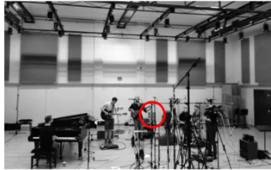
The music scene was recorded in a large recording studio (17.08×14.55×6.5 m) with a reverberation time of 1.1– 1.5 s. The ensemble recorded was a jazz group consisting of a piano, two electric guitars, a bass guitar, and drums. Close microphone signals were available for the piano, bass guitar, and one of the electric guitars. This scene presents a challenging scenario for source separation due to the reverberation time, the number of sources, and the importance of the reproduced sound timbre and quality. A diagram of the relative source positions is shown in Fig. 3. ‘Guitar 2’ (6 degrees) was used as the target for

sepa-Figure 2: Microphone array (circled) in the large studio used to record the jazz ensemble.

0! 90! Piano! Guitar 1! Bass! Drums! Guitar 2! Array! Stage area!

Figure 3: Layout of the jazz ensemble and coordinate sys-tem.

ration, with all other instruments active during the clips used for testing. In the segment analysed, the guitar was playing a lead line, which is a good example of something that a content producer may wish to re-spatialise or ma-nipulate when producing the recording.

5

RESULTS

The recordings of the scenes described above were seg-mented and the DS, SDA, MVDR, and LCMV beam-formers were applied to the signals. In the following sub-sections, the performance of each beamformer is dis-cussed, first considering the physical performance of the beamformer in terms of the beampattern, then evaluating the properties of the processed audio signals.

5.1

Implementation

To produce the output audio, finite impulse response (FIR) filters were applied to each channel, and the result-ing audio was summed at the output (i.e. a filter-and-sum structure). The array manifold vectora was calculated, in each case, based on the free-field delays expected be-tween the source position and the microphone array. Fil-ter coefficients were calculated in the frequency domain for 255 frequency bins, and FIR filters of 512 coefficients were obtained by complex conjugation, inverse Fourier transform, and the introduction of a modelling delay. Ex-periments were conducted with a sampling frequency of 16 kHz. A frequency-dependent diagonal loading param-eterεwas applied to the SDA, MVDR, and LCMV meth-ods, calculated so that the ratio between the largest eigen-value of the inverted matrix andεwas 10. This is related to the approach in ref. [32], and adjusted by experimen-tation. Coefficients for the DS method were calculated as narrowband delays. For the MVDR and LCMV methods, the covariance matricesR_xxwere calculated by splitting a clip into non-overlapping segments of 20 ms, taking the discrete-time Fourier transform, and averaging the result-ing frequency domain coefficients over all segments.

5.2

Evaluation of source weights

The first indication of the beamformer performance is given by analysing the beam pattern, using the metrics de-scribed in Sec. 3.1. As the filter coefficients were obtained using an ideal array manifold vector, their direct evalua-tion would lead to results that implied better performance than is practically realisable, due to issues including non-ideal microphone placement and noise. Therefore, to give an impression of the directivity under experimental condi-tions, the array manifold vectorawas modified by moving each microphone in thexandydirections by a random amount drawn from a normal distribution with standard deviation 5 mm, prior to the directivity pattern being cal-culated [26].

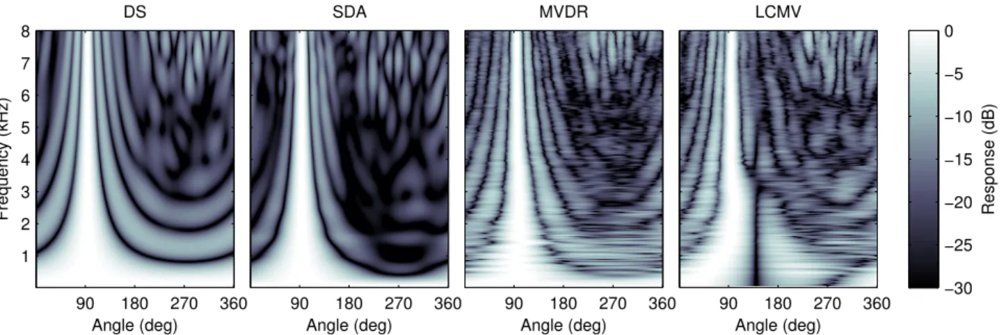
As a starting point for understanding the operation of the different approaches, consider Fig. 4, which shows di-rectivity maps for each method across azimuth and fre-quency, for the 94 degree speech target. The main fea-tures are the amount of energy in directions other than the target azimuth (quantified by DI), the width of the main

lobe (BW), the level of the highest sidelobe (SLS), and the energy at the interferer locations (AC).

The SDA exhibits the noteworthy properties of the other beamformers. There is good energy rejection from the rear of the array, the main lobe is fairly narrow and symmetric about the target direction, and there is good SLS. At higher frequencies (above 6 kHz), spatial aliasing artifacts can be noted due to the half-wavelength becom-ing shorter than the microphone spacbecom-ing. It can be seen that DS is less directive than the other methods, exhibiting a broader BW (particularly below 1 kHz) and more promi-nent spatial aliasing effects. The MVDR and LCMV di-rectivity maps have noisier responses compared with the DS and SDA, due to their weights being calculated based on measured data. The MVDR offers slightly improved directivity over DS, and the beam pattern is not symmet-ric about the target location, compared to DS and SDA. In fact, the MVDR response suppresses energy in the di-rection of the interfering source (139 degrees), while al-lowing more energy to pass in the opposite direction. The notch designed in the LCMV response can be noted across the frequency range, and the null placement significantly alters the LCMV directivity at azimuths other than the tar-get and interferer locations.

The objective measures quantify the differences be-tween the methods, and are shown in Tab. 1, considering the speech data (with errors in the microphone positions), and averaging over both target directions and 10 repeats using different 3 s segments. SDA is seen to be the op-timal method in terms of DI, BW, and SLS, whereas DS is guaranteed to give the best WNG [18] and the LCMV gives the overall best contrast. The DI and BW scores compare favourably to first-order cardioid and hypercar-dioid responses, which have DIs of 4.8 dB and 6 dB, and BWs of 131 degrees and 105 degrees, respectively [33, p.59].

The beampattern-derived scores for the music scene were comparable for DS and SDA, with small deviations due to the random microphone error. The MVDR and LCMV responses changed between the speech and mu-sic recordings due to the increased number of interfer-ing sources and reverberation. The MVDR performed comparably with the speech data, with scores of 9.4 dB, 36.9 deg., −7.2 dB, 16.9 dB, and 15.5 dB for DI, BW, SLS, AC, and WNG, respectively. On the other hand, the LCMV created a large null directed towards the other

in-Angle (deg) Frequency (kHz) DS 90 180 270 360 1 2 3 4 5 6 7 8 Angle (deg) SDA 90 180 270 360 Angle (deg) MVDR 90 180 270 360 Angle (deg) LCMV 90 180 270 360 Response (dB) −30 −25 −20 −15 −10 −5 0

Figure 4: Directivity maps of the DS, SDA, MVDR and LCMV beamformers, for target 94◦and interferer 139◦. A microphone position error with standard deviation 5 mm was applied prior to calculating the array response.

DI BW SLS AC WNG (dB) (deg.) (dB) (dB) (dB) DS 9.36 45.4 −6.44 13.3 16.8 SDA 10.6 32.2 −11.9 17.7 15.3 MVDR 9.37 34.5 −6.18 15.5 15.6 LCMV 9.21 42.6 −6.96 28.0 14.8

Table 1: Objective measures of DI, BW, SLS, and WNG, averaged over 0.1–8.0 kHz, derived from the array weights in the presence of microphone position errors. struments, at a cost of broadened main lobe and decreased WNG. The scores were 8.55 dB, 68.1 deg., −8.81 dB, 23.9 dB, and 12.7 dB for DI, BW, SLS, AC, and WNG, respectively.

5.3

Perceptual evaluation

The perceptual scores for the speech data were evaluated by taking ten non-overlapping segments (each of length 3 s) from the 30 s available. A 512 coefficient Wiener post-filter was applied to the beamformer output, and the PEASS and PESQ metrics were calculated against the close microphone reference recording. These results are recorded in Tab. 2.

The best overall performance (indicated by PEASS overall perceptual score (OPS) and PESQ) is given by DS.

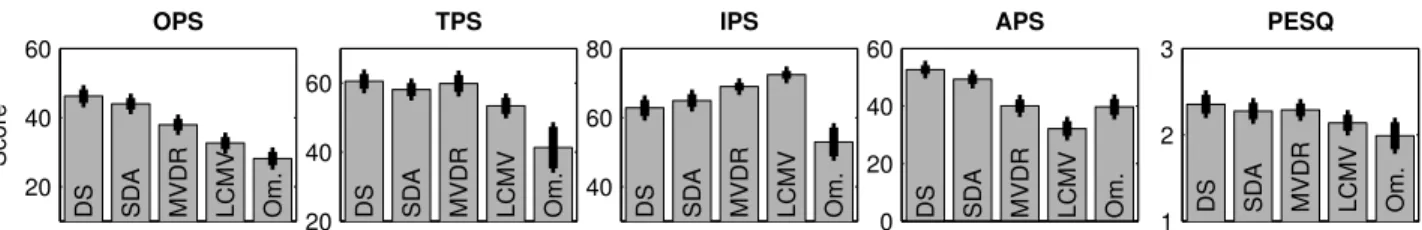
However, DS is the worst performing among the beam-formers under the interference perceptual score (IPS), which quantifies the perceptual effect of interference. It is noteworthy that the ranking among methods for the arti-fact perceptual score (APS), is opposite to that for the IPS, implying that the additional performance of the beam-formers (i.e. producing greater AC) results in audible ar-tifacts on the beamformer output. For all set of PEASS scores, the APS is the only score where the beamformers do not all improve upon the omnidirectional microphone reference. The target perceptual score (TPS) is compa-rable among DS, SDA and MVDR methods, and slightly lower for LCMV. The mean scores and 95% confidence intervals (CIs) are plotted in Fig. 5. Most notably, the dif-ferences between the OPS and IPS scores are statistically significant, with the exception of DS and SDA, whose CIs overlap in each case.

For the music scenario, the perceptual scores were cal-culated using a Matlab implementation [34] of PEAQ. The PEAQ scores were all severely degraded, giving degradation scores below−3.5 in each case (where 0 rep-resents no perceptible degradation, and −4 is the lower endpoint of the degradation scale). Using a clean guitar signal as the reference for PEAQ, the degradation scores include reverberation effects (temporal and spectral), in-terference, noise, and filter artifacts (temporal and spec-tral). Therefore, any differences between the omni ref-erence microphone and the beamformer output are

com-OPS TPS IPS APS PESQ Omni 28.1 41.3 53.0 39.7 1.99 DS 46.2 62.8 62.8 52.7 2.35 SDA 44.0 58.1 64.9 49.4 2.28 MVDR 38.0 59.9 69.0 40.1 2.29 LCMV 32.6 53.4 72.4 32.3 2.14

Table 2: Mean perceptual scores of the separated audio calculated using PEASS OPS, TPS, IPS, & APS (0–100) and PESQ (0–5) for the speech material, averaged across two simultaneous speakers separated by 45 degrees. pressed into the lower end of the scale. However, a re-duction in the level of the interfering sources was noted from informal listening, with the ranking among methods matching the speech results reported above.

6

DISCUSSION

Two kinds of directivity pattern can be obtained when using spatial filtering to perform object separation. The first is simply to focus the energy of the microphone ar-ray towards the target, which can be achieved with min-imal WNG using the DS beamformer, or with improved BW and SLS using the SDA. Alternative, the data-based MVDR and LCMV filters account for the second order statistics of the observed signals, with LCMV providing an explicit opportunity to place a null towards the inter-ferer. In general, additional directivity appears to trade off against robustness and sound quality. This can be noted by comparing the OPS, IPS and APS generated by PEASS. In fact, although all beamforming methods improve the OPS, even more significant gains could be achieved by minimizing any perceptible filtering artifacts. It is important to note that the perceptual models adopted for this work were not trained based on the kinds of artifacts introduced by beamforming. Additionally, the close microphone recordings provided as a reference were not perfectly clean, and it is unclear how this might affect the scores. Finally, the models are not perfectly suited to the subsequent adoption of the separated signals as part of a produced mix. It is likely that in such a scenario, some interference and artifacts could be masked and the overall effect achieved by re-mixing the stems could have

a significant impact by giving greater control to the pro-ducer. Future perceptual models designed for re-mixing may take these effects better into account.

The beamforming approaches go some way to isolat-ing individual sound objects from the scenes, especially in terms of reducing the interference due to non-target sources. In addition to reducing the beamforming arti-facts, improvements may be derived by adopting higher-order statistics to better exploit the number of capsules in the array.

7

SUMMARY

Acquisition of audio signals for object-based production is a relatively new topic. In this paper, we proposed spa-tial filtering techniques applied to a higher-order micro-phone array as a potential method for object separation, i.e. segmenting a scene into a number of individual audio streams. DS, SDA, MVDR and LCMV filters were ap-plied to a 48 channel array, with recordings of speech and music signals. The beamformers were found to improve the overall perceptual impression compared to a reference omnidirectional microphone, although the isolation of the target sounds was limited compared to the reference sig-nals captured with close microphones.

8

ACKNOWLEDGEMENTS

The authors would like to thank the voice actors and mu-sicians who performed for the capture sessions. This re-search was supported by the EPSRC Programme Grant S3A: Future Spatial Audio for an Immersive Listener Ex-perience at Home (EP/L000539/1), and the BBC as part of the Audio Research Partnership.

References

[1] B. Shirley, R. Oldfield, F. Melchior, and J.-M. Batke, “Platform independent audio,” inMedia Production, De-livery and Interaction for Platform Independent Systems, pp. 130–165, John Wiley & Sons, 2014.

[2] F. Rumsey,Spatial audio. Focal Press, Oxford, UK, 2001. [3] K. Hamasaki and K. Hiyama, “Reproducing spatial im-pression with multichannel audio,” in24th AES Int. Conf.

20 40 60 OPS Score DS SDA MVDR LCMV Om. 20 40 60 TPS DS SDA MVDR LCMV Om. 40 60 80 IPS DS SDA MVDR LCMV Om. 0 20 40 60 APS DS SDA MVDR LCMV Om. 1 2 3 PESQ DS SDA MVDR LCMV Om.

Figure 5: Perceptual scores and 95% confidence intervals of the separated audio calculated using PEASS OPS, TPS, IPS, & APS (0–100) and PESQ (0–5) for the speech material, averaged across two simultaneous speakers separated by 45 degrees.

on Multichannel Audio, The New Reality. Alberta, Canada, 26-28 June, 2003.

[4] A. Farina, S. Campanini, L. Chiesi, A. Amendola, and L. Ebri, “Spatial sound recording with dense microphone arrays,” in55th AES Int. Conf. on Spatial Audio. Helsinki, Finland, 27-29 August, 2014.

[5] B. D. Van Veen and K. M. Buckley, “Beamforming: A ver-satile approach to spatial filtering,”IEEE assp magazine, vol. 5, no. 2, pp. 4–24, 1988.

[6] Y. Huang, J. Chen, and J. Benesty, “Immersive audio schemes,” IEEE Signal Processing Magazine, vol. 28, no. 1, pp. 20–32, 2011.

[7] B. Rafaely, Y. Peled, M. Agmon, D. Khaykin, and E. Fisher, “Spherical microphone array beamforming,” in Speech Processing in Modern Communication, pp. 281– 305, Springer, 2010.

[8] E. Hulsebos, T. Schuurmans, D. de Vries, and R. Boone, “Circular microphone array for discrete multichannel au-dio recording.,” in114th AES Convention, Amsterdam, 22-25 March, 2003.

[9] F. Pinto and M. Vetterli, “Space-time-frequency process-ing of acoustic wave fields: Theory, algorithms, and appli-cations,”IEEE Trans. Sig. Proc., vol. 58, no. 9, pp. 4608– 4620, 2010.

[10] L. Remaggi, P. J. B. Jackson, and P. Coleman, “Estimation of room reflection parameters for a reverberant spatial au-dio object,” in138th AES Convention, Warsaw, 7-10 May, 2015.

[11] J. Chen, J. Benesty, and Y. A. Huang, “Time delay es-timation in room acoustic environments: an overview,” EURASIP Journal on Advances in Signal Processing, vol. 2006, pp. 1–19, 2006.

[12] J. P. Dmochowski and J. Benesty, “Steered beamform-ing approaches for acoustic source localization,” in

Speech processing in modern communication, pp. 307– 337, Springer, 2010.

[13] V. Pulkki, “Spatial sound reproduction with directional au-dio coding,” Journal of the Audio Engineering Society, vol. 55, no. 6, pp. 503–516, 2007.

[14] R. Oldfield, B. Shirley, and J. Spille, “An object-based audio system for interactive broadcasting,” in137th AES Convention, Los Angeles, CA, 9-12 Oct, 2014.

[15] J. Herre, J. Hilpert, A. Kuntz, and J. Plogsties, “MPEG-H audio — the new standard for universal spatial/3D audio coding,”J. Audio Eng. Soc, vol. 62, no. 12, pp. 821–830, 2015.

[16] S. F¨ug, A. H¨olzer, C. Borß, C. Ertel, M. Kratschmer, and J. Plogsties, “Design, coding and processing of metadata for object-based interactive audio,” in137th AES Conven-tion, Los Angeles, CA, 9-12 Oct, 2014.

[17] E. A. Habets, J. Benesty, S. Gannot, and I. Cohen, “The MVDR beamformer for speech enhancement,” in Speech Processing in Modern Communication, pp. 225– 254, Springer, 2010.

[18] M. R. Bai, J.-G. Ih, and J. Benesty,Acoustic Array Sys-tems: Theory, Implementation, and Application. Wiley-IEEE press, 2014.

[19] C. Pan, J. Chen, and J. Benesty, “Performance study of the MVDR beamformer as a function of the source incidence angle,”IEEE/ACM Trans. Audio, Speech and Lang. Proc., vol. 22, pp. 67–79, Jan. 2014.

[20] M. R. Bai and C.-C. Chen, “Application of convex opti-mization to acoustical array signal processing,”J. Sound Vib., vol. 332, no. 25, pp. 6596–6616, 2013.

[21] E. Habets, J. Benesty, I. Cohen, S. Gannot, and J. Dmo-chowski, “New insights into the MVDR beamformer in room acoustics,”IEEE Trans. Audio Speech Lang. Proc., vol. 18, pp. 158–170, Jan 2010.

[22] M. Souden, J. Benesty, and S. Affes, “A study of the lcmv and mvdr noise reduction filters,”Signal Processing, IEEE Transactions on, vol. 58, no. 9, pp. 4925–4935, 2010. [23] O. Thiergart and E. Habets, “An informed LCMV filter

based on multiple instantaneous direction-of-arrival es-timates,” in IEEE Int. Conf. Acoust. Speech Sig. Proc. (ICASSP). Vancouver, Canada, 26-31 May, pp. 659–663, May 2013.

[24] O. Thiergart and E. Habets, “Extracting reverberant sound using a linearly constrained minimum variance spatial fil-ter,”IEEE Signal Processing Letters, vol. 21, pp. 630–634, May 2014.

[25] W. M. Humphreys Jr, T. F. Brooks, W. W. Hunter Jr, and K. R. Meadows, “Design and use of microphone di-rectional arrays for aeroacoustic measurements,” in36th Aerospace Sciences Meeting and Exhibit, Jan 12-15 1998, Reno, NV, 1998.

[26] P. Coleman, P. J. B. Jackson, M. Olik, M. Møller, M. Olsen, and J. A. Pedersen, “Acoustic contrast, planarity and robustness of sound zone methods using a circular loudspeaker array,”J. Acoust. Soc. Am., vol. 135, no. 4, pp. 1929–1940, 2014.

[27] E. Vincent, R. Gribonval, and C. F´evotte, “Performance measurement in blind audio source separation,” IEEE Trans. Audio Speech Lang. Proc., vol. 14, no. 4, pp. 1462– 1469, 2006.

[28] V. Emiya, E. Vincent, N. Harlander, and V. Hohmann, “Subjective and objective quality assessment of audio source separation,”IEEE Trans. Audio Speech Lang. Proc., vol. 19, no. 7, pp. 2046–2057, 2011.

[29] A. W. Rix, J. G. Beerends, M. P. Hollier, and A. P. Hek-stra, “Perceptual evaluation of speech quality (PESQ) - a new method for speech quality assessment of telephone networks and codecs,” inIEEE Int. Conf. Acoust. Speech Sig. Proc. (ICASSP). Salt Lake City, UT, 7-11 May, vol. 2, pp. 749–752, IEEE, 2001.

[30] T. Thiede, W. C. Treurniet, R. Bitto, C. Schmidmer, T. Sporer, J. G. Beerends, and C. Colomes, “PEAQ—the ITU standard for objective measurement of perceived au-dio quality,”J. Audio Eng. Soc, vol. 48, no. 1/2, pp. 3–29, 2000.

[31] P. J. B. Jackson, F. Jacobsen, P. Coleman, and J. A. Peder-sen, “Sound field planarity characterized by superdirective beamforming,” inProc. Meetings Acoust., 21st ICA Mon-treal, 2-7 June, 2013.

[32] O. Kirkeby and P. A. Nelson, “Reproduction of plane wave sound fields,”J. Acoust. Soc. Am., vol. 94, no. 5, pp. 2992– 3000, 1993.

[33] Y. Huang and J. Benesty, eds.,Audio Signal Processing for Next-Generation Multimedia Communication Systems. Springer, 2004.

[34] P. Kabal, “An examination and interpretation of ITU-R BS. 1387: Perceptual evaluation of audio quality,” TSP Lab Technical Report, Dept. Electrical & Computer Engineer-ing, McGill University, pp. 1–89, 2002.