Strategic Infrastructure Planning for Autonomous Vehicles

by Zhaocai Liu

A dissertation submitted in partial fulfillment of the requirements for the degree

of

DOCTOR OF PHILOSOPHY in

Civil and Environmental Engineering

Approved:

______________________ ____________________

Ziqi Song Patrick Singleton

Major Professor Committee Member

______________________ ____________________

Michelle Mekker Haitao Wang

Committee Member Committee Member

______________________ ____________________

Marvin W. Halling Richard Inouye, Ph.D.

Committee Member Vice Provost of Graduate Studies

UTAH STATE UNIVERSITY Logan, Utah

Copyright © Zhaocai Liu 2020 All Rights Reserved

ABSTRACT

Strategic Infrastructure Planning for Autonomous Vehicles by

Zhaocai Liu

Utah State University, 2020

Major Professor: Dr. Ziqi Song

Department: Civil and Environmental Engineering

Emerging autonomous vehicle (AV) technology is expected to bring dramatic societal, environmental, and economic benefits. To promote the realization of the potential benefits of AV technology, this dissertation aims at investigating the modeling and optimization of network infrastructure modification and enhancement planning for autonomous vehicles. This dissertation first examines the traffic assignment and congestion pricing problems in a network with mixed AVs and human-driven vehicles (HVs). The impact of AVs on road capacity and drivers’ value of travel time is explicitly considered. Numerical results reveal a paradoxical phenomenon that the adoption of AVs may increase network congestion under certain situations. The effectiveness of

congestion pricing is also demonstrated with numerical studies.

This dissertation then studies the optimization problem for dedicating lanes for priority or exclusive use by AVs. Deploying dedicated lanes for autonomous vehicles is foreseen as an effective way to amplify the road-capacity-improvement benefit from autonomous vehicles and boost the market penetration of autonomous vehicles. However, dedicated autonomous vehicle lanes may be underutilized when autonomous vehicle

flows are relatively low. This dissertation introduces a new form of managed lanes for autonomous vehicles, designated as autonomous-vehicle/toll lanes, which are freely accessible to autonomous vehicles while allowing human-driven vehicles to utilize the lanes by paying a toll. Numerical results demonstrate that the joint use of dedicated autonomous vehicle lanes and autonomous-vehicle/toll lanes can better improve the system efficiency of transportation networks with mixed human-driven vehicles and autonomous vehicles.

This dissertation further explores an infrastructure-enabled autonomous driving system. The system combines vehicles and infrastructure in the realization of autonomous driving. Equipped with roadside sensor and control systems, a regular road can be

upgraded into an automated road providing autonomous driving service to vehicles. Vehicles only need to carry minimum required on-board devices to enable their

autonomous driving on an automated road. The costs of vehicles can thus be significantly reduced. Moreover, the liability associated with autonomous driving can now be shared by vehicle makers, infrastructure providers, and/or some third-party players. A network modeling framework is proposed for the evaluation and planning of the infrastructure-enabled autonomous driving system. Numerical studies demonstrate that the

infrastructure-enabled autonomous driving system is of great potential in promoting the adoption of autonomous driving technology.

PUBLIC ABSTRACT

Strategic Infrastructure Planning for Autonomous Vehicles Zhaocai Liu

Compared with conventional human-driven vehicles (HVs), AVs have various potential benefits, such as increasing road capacity and lowering vehicular fuel

consumption and emissions. Road infrastructure management, adaptation, and upgrade plays a key role in promoting the adoption and benefit realization of AVs. This

dissertation investigated several strategic infrastructure planning problems for AVs. First, it studied the potential impact of AVs on the congestion patterns of transportation

networks. Second, it investigated the strategic planning problem for a new form of managed lanes for autonomous vehicles, designated as autonomous-vehicle/toll lanes, which are freely accessible to autonomous vehicles while allowing human-driven vehicles to utilize the lanes by paying a toll. This new type of managed lanes has the potential of increasing traffic capacity and fully utilizing the traffic capacity by selling redundant road capacity to HVs. Last, this dissertation studied the strategic infrastructure planning problem for an infrastructure-enabled autonomous driving system. The system combines vehicles and infrastructure in the realization of autonomous driving. Equipped with roadside sensor and control systems, a regular road can be upgraded into an

automated road providing autonomous driving service to vehicles. Vehicles only need to carry minimum required on-board devices to enable their autonomous driving on an automated road. The costs of vehicles can thus be significantly reduced.

To my parents, who gave me a love of life

To my wife Yi He, who gave me a life of love

ACKNOWLEDGMENTS

I would like to express my deepest gratitude and appreciation to my advisor Dr. Ziqi Song for his guidance and support during my studies. It is a great honor for me to be his first Ph.D. student. He is a patient teacher, a supportive friend, and a talented and passionate researcher. He introduced me to this amazing venue of transportation research as my career, guided me through the academic jungle, and sharped my views towards transportation systems.

I would also like to thank Dr. Patrick Singleton, Dr. Michelle Mekker, Dr. Haitao Wang, and Dr. Marvin W. Halling, for serving on my dissertation committee and giving me valuable comments and suggestions on my dissertation research.

I would like to acknowledge U.S. Department of Energy, Utah Department of Transportation, Mountain-Plains Consortium, and Transportation Research Center for Livable Communities for providing financial support.

CONTENTS Page ABSTRACT ... III PUBLIC ABSTRACT ... V ACKNOWLEDGMENTS ... VII LIST OF TABLES ... XI LIST OF FIGURES ... XIII

CHAPTER ... 1 1 INTRODUCTION ... 1 1.1 Background ... 1 1.2 Research objectives ... 4 1.3 Dissertation organization ... 6 2 LITERATURE REVIEW ... 7

2.1 Review of network equilibrium and congestion pricing studies ... 7

2.2 Review of lane management studies ... 11

2.3 Review of infrastructure-enabled autonomous driving studies ... 13

3 USER EQUILIBRIUM AND CONGESTION PRICING PROBLEMS FOR THE MIXED AUTONOMOUS VEHICLES AND HUMAN-DRIVEN VEHICLES ... 16

3.1 User equilibrium problem in networks with mixed HVs and AVs ... 17

3.1.1 Basic considerations and notations ... 17

3.1.2 Traffic capacity for links with mixed flows of HVs and AVs ... 18

3.1.3 HV equivalents for AVs ... 22

3.1.4 User equilibrium model ... 24

3.1.5 Solution existence and uniqueness for the user equilibrium model ... 25

3.1.6 Solution algorithm ... 32

3.1.6.1 Diagonalization algorithm ... 32

3.1.6.2 A gap function approach ... 34

3.1.7 Quantifying network delay under best and worst cases ... 35

3.1.8 Numerical studies ... 36

3.2 System optimum and first-best pricing ... 43

3.2.1 Tolled user equilibrium flow distribution ... 44

3.2.2 System optimum in time units and pricing for user equilibrium ... 47

3.2.3 System optimum in monetary units and pricing for user equilibrium ... 51

3.3 Robust congestion pricing ... 54

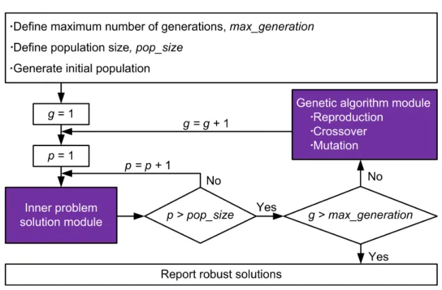
3.3.2 Solution algorithm ... 57

3.3.2.1 Inner problem solution module ... 58

3.3.2.2 Genetic algorithm module ... 59

3.3.3 Numerical studies ... 61

3.4 Summary ... 64

4 STRATEGIC PLANNING OF DEDICATED AUTONOMOUS VEHICLE LANES AND AUTONOMOUS VEHICLE/TOLL LANES IN TRANSPORTATION NETWORKS... 66

4.1. Potential benefits of AV lanes and AVT lanes ... 67

4.2 UE model with AV/AVT lanes ... 69

4.3 Deployment model ... 73

4.4 Solution algorithm ... 76

4.4.1 Inner problem solution module ... 76

4.4.2 Genetic algorithm module ... 79

4.5 Numerical studies ... 80

4.5.1 The Nguyen-Dupuis network ... 81

4.5.2 The Sioux Falls network ... 86

4.6 Summary ... 89

5 STRATEGIC PLANNING OF AUTOMATED ROADS FOR INFRASTRUCTURE-ENABLED AUTONOMOUS VEHICLES ... 91

5.1 Network equilibrium model ... 92

5.1.1 UE conditions ... 93

5.1.2 Road users’ vehicle type choice ... 98

5.1.3 Variational inequality formulation ... 99

5.1.4 Solution algorithm ... 105

5.1.5 Numerical examples ... 106

5.2 Deployment of automated roads ... 112

5.2.1 Model formulation ... 112

5.2.2 Solution algorithm ... 113

5.2.3 Numerical Studies ... 116

5.2.3.1 Nguyen-Dupuis network ... 117

5.2.3.2 Sioux Falls network ... 118

5.3 Model extensions ... 124

5.3.1 Network equilibrium model considering service charges and inconvenience costs ... 126

5.3.1.1 Driving mode choice of IEAV users on automated links ... 128

5.3.1.2 Proportion of autonomous driving vehicles in mixed traffic and travel time function reformulation ... 140

5.3.1.3 Formulation of UE model ... 142

5.3.1.5 Numerical studies ... 154

5.3.2 Vehicle choice model ... 158

5.3.3 Time-dependent deployment model of automated roads ... 162

5.4 Summary ... 164

6 CONCLUSIONS AND FUTURE WORKS ... 169

6.1 Summary of major findings ... 169

6.2 Future research ... 172

REFERENCES ... 174

LIST OF TABLES

Table Page

3-1: Flow distributions and link travel times for the toy network in the first

scenario ... 30

3-2: Flow distributions and link travel times for the toy network in the second scenario ... 31

3-3: UE solutions for Scenario 2 with PR = 0 and PR = 1 ... 41

3-4: Flow distributions for Scenario 3 with PR = 0.7 ... 43

3-5: Link characteristics of the Nguyen-Dupuis network ... 62

3-6: Robust toll design in the Nguyen-Dupuis network ... 64

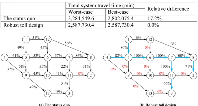
3-7: System performances in status quo condition and robust toll design ... 64

4-1: Efficiency of road segment (1, 2) under different scenarios ... 69

4-2: Link characteristics of the Nguyen-Dupuis network with candidate AV/AVT links ... 82

4-3: Link pairs in the Nguyen-Dupuis network ... 82

4-4: Robust optimal deployment of AV/AVT lanes in the Nguyen-Dupuis. network ... 83

4-5: Travel time comparison between AVT links and their paired regular links ... 84

4-6: System performances in status quo condition and robust deployment plan ... 86

4-7: Comparison of worst-case equilibrium O-D travel costs ... 86

4-8: Link characteristics of the Sioux Falls network with candidate AV/AVT links ... 87

4-9: Total O-D demands of AVs and HVs of the Sioux Falls network (veh/h) ... 88

4-10: Robust deployment of AV/AVT lanes for the Sioux Falls network ... 89

5-1: Link characteristics of the Nguyen-Dupuis network ... 107

5-2: Equilibrium O-D travel cost and demand by class ... 109

5-3: Equilibrium market shares under different IEAV prices ... 109

Table Page 5-5: Comparison between status quo and optimal design for the

Nguyen-Dupuis network ... 118

5-6: Link characteristics of the Sioux Falls network for deployment of. automated roads ... 119

5-7: O-D demands of the Sioux Falls network for deployment of automated roads (veh/h) ... 120

5-8: Total market shares and total user benefit in the status quo and in the. optimal deployment plan ... 121

5-9: Market shares in status quo and in optimal deployment plan ... 121

5-10: Travel costs in status quo and in optimal deployment plan ... 123

5-11: A new set of link characteristics of the Nguyen-Dupuis network ... 154

5-12: Equilibrium O-D travel cost by vehicle class ... 155

5-13: Equilibrium O-D travel cost comparison between the scenarios with and without automated links ... 157

LIST OF FIGURES

Figure Page

3-1. Illustration of inter-vehicle headways. ... 19

3-2. A toy network with one O-D pair and three links. ... 29

3-3. A toy network with one O-D pair and five links. ... 37

3-4. System travel times for Scenario 1. ... 39

3-5. System travel times for Scenario 2. ... 41

3-6. Comparison of system performances for Scenario 3. ... 44

3-7. Flowchart of the genetic-algorithm-based approach. ... 57

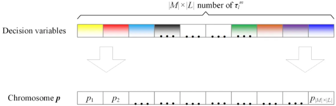
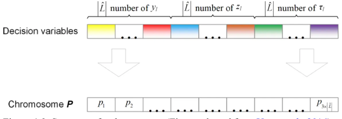
3-8. Structure of a chromosome (Figure adapted from Yang et al., 2016). ... 60

3-9. Nguyen-Dupuis network with candidate toll links. ... 62

3-10. AV flow ratios in status quo condition and robust toll design. ... 64

4-1. A road segment with two lanes. ... 68

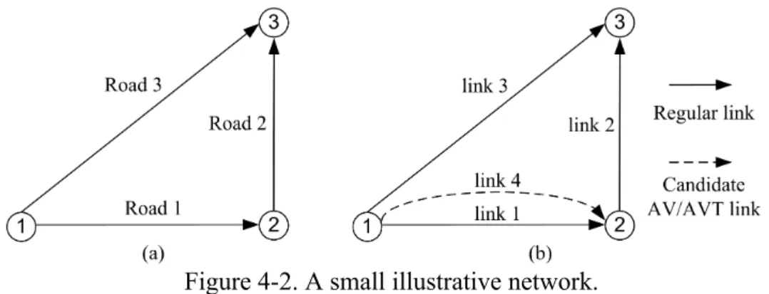
4-2. A small illustrative network. ... 70

4-3. Structure of a chromosome (Figure adapted from Yang et al., 2016). ... 80

4-4. Nguyen-Dupuis network with candidate AV/AVT links. ... 82

4-5. Robust optimal deployment of AV/AVT lanes in the Nguyen-Dupuis. network. ... 84

4-6. Sioux Falls network with candidate AV/AVT links. ... 87

5-1. Nguyen-Dupuis network with automated links. ... 108

5-2. Equilibrium total market shares under different value of time ... 111

5-3. Sioux Falls network for the deployment of automated roads ... 120

5-4. Deployment of automated links in Sioux Falls network ... 123

5-5. Different combinations of two consecutive links ... 131

5-6. A toy network with four nodes ... 132

5-7. Illustration of automated road segments ... 135

5-8. Illustration of the network expansion ... 151

INTRODUCTION 1.1 Background

Compared with conventional human-driven vehicles (HVs), autonomous vehicles (AVs) have various potential benefits, such as reducing deadly crashes, increasing road capacity, lowering vehicular fuel consumption and emissions, and providing critical mobility to the elderly and disabled (Fagnant and Kockelman, 2015; Chen et al., 2016; Levin and Boyles, 2016a,b; Bagloee et al., 2016; Meyer et al., 2017; Pan et al., 2019). Although commercial AVs have not been offered in the market, recent progress suggests they are on the horizon. In partnership with Lyft, nuTonomy, a software company, has launched the nation’s first self-driving ridesharing service in Boston in December 2017 (nuTonomy, 2018). At the end of 2018, Waymo, formerly the Google self-driving car project, launched its first commercial self-driving service in the Metro Phoenix area, Arizona (Waymo, 2018a). Moreover, Waymo plans to add up to 20,000 I-PACE vehicles to its fleet in the next few years (Waymo, 2019). Many automakers such as Nissan (Nissan, 2017), Honda (Honda, 2019), and Toyota (TOYOTA, 2019) have announced their intentions to provide commercially-viable autonomous-driving capabilities by 2020 in some of their vehicle models. Many researchers (e.g., Litman, 2017; Bansal and Kockelman, 2017; Talebian and Mishra, 2018) have predicted that AVs will constitute a significant or even dominant portion of the vehicle market in the next few decades. Therefore, it is imperative to modify existing travel demand and network flow models to capture the characteristics of AVs.

have smaller time headways than HVs and thus may increase road capacity. This benefit of AVs has been demonstrated by both simulation (e.g., Shladover et al., 2012; Ntousakis et al., 2015) and analytical modeling analyses (e.g., Levin and Boyles, 2015; van den Berg and Verhoef, 2016). The impact of AVs on traffic capacity will inevitably influence the traffic flow distributions and congestion patterns of networks with AVs. Moreover, by allowing drivers to conduct other activities, AVs may also reduce the value of travel time (VOT) of drivers (Le Vine et al., 2015; van den Berg and Verhoef, 2016; Noruzoliaee et al., 2018). The VOT change of drivers will influence their reactions to congestion pricing.

Deploying dedicated lanes for AVs is foreseen as an effective way to amplify the capacity-improvement benefit from AVs and boost the market penetration of AVs (Chen et al., 2016; Chen et al., 2019; Ghiasi et al., 2017; Lamotte et al., 2017; Lu et al., 2019). However, dedicated AV lanes may be underutilized when AV flows are relatively low (Chen et al., 2016). We thus consider a new form of managed lanes for AVs, designated as autonomous-vehicle/toll (AVT) lanes, which are freely accessible to AVs while allowing HVs to utilize the lanes by paying a toll. The idea of AVT lanes is derived from high-occupancy vehicle (HOV) lanes and high-occupancy/toll (HOT) lanes (Fielding and Klein, 1993;Dahlgren, 2002). The joint use of dedicated AV lanes and AVT lanes can better improve the system efficiency of transportation networks with mixed AV and HV traffic.

Currently the development of autonomous driving is focusing on autonomous vehicle (AV) technology and mainly led by the private sector, which includes technology

companies such as Google and Baidu, automakers such as Audi, Toyota, Ford, and Volvo, and transportation network companies such as Uber, Lyft, and DiDi. As of July 2018, Google’s AV fleet has self-driven over eight million miles on public roads

(Waymo, 2018b), and numerous manufacturers, including BMW, Nissan, Ford, General Motors, Tesla, Mercedes-Benz, and Bosch, have begun testing their prototype AVs (Wang, 2018).

However, focusing on AV technology alone may potentially slow the penetration of AVs and consequently slowing the realization of societal benefits of AVs. In order to safely drive itself in various road environment, an AV needs to be equipped with

expensive sensor systems and additional hardware and software. The high cost of AVs can be a significant barrier to their broad adoption (Fagnant and Kockelman, 2015; Jun and Markel, 2017). Moreover, if autonomous driving only relies on AVs, the AV makers will be saddled with both the responsibility and liabilities associated with the traditional capabilities of the vehicle, but also those associated with functions that human beings routinely perform (Gopalswamy and Rathinam, 2018). The liability threats associated with AVs will be an important and potentially limiting consideration for AV makers, and have the potential to present a significant deterrent to the development of AVs (Marchant and Lindor, 2012). Integrating transportation infrastructure enhancement into the

realization of autonomous driving can potentially promote the development and adoption of AVs (Rebsamen et al., 2012; Horst et al., 2016; Jun and Markel, 2017; Ran et al., 2019a,b; Sanchez et al., 2016). With the development of vehicle to vehicle and vehicle to infrastructure technologies, researchers have suggested that an infrastructure-enabled or

infrastructure-based autonomous driving system provides a promising alternative to the development of autonomous driving (Gopalswamy and Rathinam, 2018; Ran et al., 2019a,b).

1.2 Research objectives

The main objective of this dissertation is to investigate the modeling and

optimization of network infrastructure modification and enhancement planning for AVs. More specifically, this dissertation will make the following contributions.

First, this dissertation investigates traffic assignment and congestion pricing problems in a network with mixed AVs and HVs. It is assumed that both HVs and AVs will selfishly choose their routes to minimize their individual travel costs, i.e., they follow the user equilibrium routing principle. Considering headway realizations in different AV technology scenarios, this dissertation analyzes the impact of AVs on road traffic capacity and provides an analytical capacity model for road segments with mixed HV and AV flows. This dissertation formulates a user equilibrium traffic assignment model, proves the solution existence of the user equilibrium, and establishes the uniqueness conditions for the solutions of link travel time and system delay. This dissertation then investigates the system optimal, the first-best and second-best congestion pricing problems in networks with mixed HV and AV flows.

Second, this dissertation proposes the concept of autonomous vehicle/toll (AVT) lanes, which is a promising alternative to dedicated AV lanes when AV flows are

relatively low. A network modeling framework is then proposed to determine the optimal deployment of dedicated AV lanes and AVT lanes in a transportation network with

mixed HV and AV flows. Considering the user equilibrium problem with mixed HVs and AVs may have non-unique flow distribution and system delay, this dissertation proposed a robust optimal deployment model to deploy dedicated AV lanes and AVT lanes in a manner that minimizes the social cost under the worst-case flow distribution. The robust optimal deployment model is formulated as a generalized semi-infinite min-max program and is solved using a genetic-algorithm-based approach.

Last, this dissertation explores the potential of an infrastructure-enabled autonomous driving system and develop a modeling framework for the planning and evaluation of such a system. It is envisioned that there will three major types of vehicles in the market: conventional human-driven vehicles (HVs), infrastructure-independent autonomous vehicles (IIAVs), and infrastructure-enabled autonomous vehicles (IEAVs). This dissertation will develop a new network equilibrium model to describe road users’ vehicle type and route choice behaviors in a transportation network with automated roads. The model will consider two special characteristics of IEAVs: (1) IEAVs are driven by human drivers on regular roads and will be driven autonomously on automated roads; (2) IEAV users will experience different value of travel time on regular and

automated roads. Based on the proposed network equilibrium model, this dissertation will further investigate the strategic planning of automated roads in a general transportation network. To the best of our knowledge, this study will be the first in the literature that develops a modeling framework for the planning and evaluation of the infrastructure-enabled autonomous driving system in a general transportation network.

1.3 Dissertation organization

The remainder of this dissertation is organized as follows. Chapter 2 reviews related work and highlights how this dissertation can contribute to the existing literature. Chapter 3 first investigates the network equilibrium problem in networks with mixed HVs and AVs. The system optimal, first-best and second-best pricing problems are then studied. Chapter 4 formulates the robust optimization model for the deployment of dedicated AV lanes and AVT lanes and proposes a genetic-algorithm-based algorithm to solve it. Numerical studies are provided to demonstrate the model and the solution algorithm. Chapter 5 develops a network modeling framework for the planning and evaluation of the infrastructure-based autonomous driving system. Chapter 6 concludes the dissertation and discuss future research directions.

CHAPTER 2

LITERATURE REVIEW

2.1 Review of network equilibrium and congestion pricing studies

Several studies have investigated the network equilibrium problem involving AVs. Chen et al. (2016) proposed a multi-class network equilibrium model for a

transportation network with dedicated AV lanes and mixed AV and HV flows. The model assumes that AVs will significantly improve road capacity on dedicated AV lanes,

whereas they will have no influence on the traffic capacity of roads with mixed flows.

Chen et al. (2017b) further developed a network equilibrium model for a transportation network with dedicated AV zones and mixed AV and HV flows. In the model, travelers are assumed to minimize their perceived travel times when they make route choices. Perceived travel times are actual trip times for HV users, while for AV users they represent the actual travel times spent outside of the dedicated AV zones plus perceived marginal travel times within the dedicated AV zones (i.e., AVs are controlled by a central manager and follow a system-optimum (SO) routing principle within the dedicated AV zones). The model also assumes that AVs will improve road capacity within the

dedicated AV zones while having no influence on road capacity outside the dedicated AV zones. Considering mixed AV and HV travel demands, Jiang (2017) proposed a

combined mode split and traffic assignment model. The model assumes that AVs and HVs travel on separate lanes throughout the network and respectively follow the Cournot-Nash (CN) principle (i.e., AVs try to minimize their total travel cost through cooperation) and the user equilibrium (UE) principle when choosing routes. Based on the

assumption that a central agent can fully control a fraction of the AV fleet in a network,

Zhang and Nie (2018) proposed a mixed network equilibrium model with multi-class users. The model assumes that users who are not controlled by the central agent will try to minimize their own travel time through selfishly choosing their routes (i.e., following the UE routing principle), whereas users who are controlled by the central agent will try to minimize total system travel time through cooperative routing behavior (i.e., following the SO routing principle). The above studies either do not consider the case with mixed AV and HV flows (i.e., Jiang, 2017) or neglect the potential impact of AVs on the

capacity of roads with mixed flows (i.e., Chen et al., 2016, 2017b; Zhang and Nie, 2018). However, because it will be many years before AVs are widely adopted and it may be impractical to completely separate AV and HV flows throughout a transportation network, a heterogeneous traffic flow consisting of both AVs and HVs will inevitably exist for a long time. In addition, as reported by many studies (e.g., Ghiasi et al., 2017; Bierstedt et al., 2014; Shladover, 2012), the potential impact of AVs on the capacity of roads with mixed AV and HV flows can be significant. Therefore, it is of great

theoretical and practical importance to study the network equilibrium problem with mixed AV and HV flows and to specifically consider the impact of AVs on road capacity with mixed traffic.

Levin and Boyles (2015) proposed a multiclass user equilibrium model for traffic assignment in a network with mixed HVs and AVs. They adopted the well-known Bureau of Public Roads (BPR) travel time function in their model. They considered that AVs will have smaller headways than HVs and the traffic capacity of a road is a function of the

proportion of AVs on the road. Mehr and Horowitz (2019) developed a user equilibrium model for a network with mixed autonomy. They also adopted the BPR travel time function and considered that the traffic capacity of a road is a function of the proportion of AVs on the road. However, the road capacity function adopted in both Levin and Boyles (2015) and Mehr and Horowitz (2019) only considered two types of deterministic time headways and neglected the stochasticity of mixed traffic (Ghiasi et al., 2017).

Only a limited number of studies have investigated the congestion pricing problems in networks with mixed traffic of both HVs and AVs. Ye and Wang (2018)

proposed a bi-level network design model compromising dedicated AV links and congestion pricing to reduce traffic congestion. They assume that congestion pricing is only implemented for HVs. They also assume that dedicated AV links can only be accessed by AVs and will have significantly increased capacity, whereas regular links will have unchanged capacity although they will be used by mixed HVs and AVs. As discussed above, the impact of AVs on the capacity of roads with mixed traffic may be significant and thus should not be neglected. Tscharaktschiew and Evangelinos (2019)

studied the interactions between the transition in automated driving capabilities on road congestion pricing. They considered the interdependencies between traffic flow, the choice level of autonomous driving, effective road capacity, and marginal travel cost. To make the analysis simple and clear, they adopted the classical continuous static model of traffic congestion pricing. They considered a single origin-destination pair connected by a single road in their numerical study. Their study focuses on the economic analysis of congestion pricing rather than network-level congestion pricing design. Recently,

considering different potential future scenarios with different market penetration of AVs and shared AVs, Simoni et al. (2019) developed multiple congestion pricing and tolling strategies and investigated their effects on the Austin, Texas network conditions and traveler welfare, using the agent-based simulation model MATsim (www.matsim.org). An agent-based model allows a higher level of realism compared to conventional static traffic assignment model because it is possible to explicitly model several factors concerning transportation demand and traffic. However, it requires demanding computational effort.

Also worth noting here are a few recent studies that propose new and futuristic tolling schemes in a connected and automated vehicles environment. Basar and Cetin (2017) proposed a novel tolling system based on descending price auction. They conducted an online survey to assess the public acceptance of the auction-based tolling systems over current dynamic and fixed tolling methodologies on highways. Based on the analysis of the survey data and, the authors found that, among those who are familiar with the current tolling methods, there is no outright rejection of the new tolling method. In addition, they found that, compared to fixed tolling, the new tolling method generates more revenue and improves the capacity utilization of the toll road. Sharon et al. (2017)

presented a mechanism for setting dynamic and adaptive tolls denoted Delta-toll for connected and automated vehicles. The Delta-toll is a model-free adaptive tolling scheme which only requires travel time observations on links. They showed the effectiveness of Delta-tolling using traffic simulators. They also proved that the Delta-tolling will yield

system optimal flow for the special case of the static network equilibrium model with BPR-style delay functions.

2.2 Review of lane management studies

Traffic capacity analysis for a road with mixed AVs and HVs have been

conducted in many studies (e.g., Shladover et al., 2012; Ntousakis et al., 2015; Levin and Boyles, 2015; van den Berg and Verhoef, 2016). Based on the anticipation that AVs will have reduced time headways when following other vehicles, majority of these studies concluded that traffic capacity would increase substantially with the increase of the AV flow proportion. A number of studies (e.g., Chen et al., 2016; Ghiasi et al., 2017;

Talebpour et al., 2017; Ye and Yamamoto, 2018) have indicated that reserving dedicated lanes for AVs can possibly further amplify their benefits in improving traffic capacity.

Tientrakool et al. (2011) showed that, due to the benefits of reduced inter-vehicle safe distance, the capacity of lanes used by pure AV flows will approximately become tripled compared to the capacity in the case of pure HV flows. Using microscopic simulation,

Talebpour et al. (2017) investigated the impacts of reserved lanes for AVs on congestion and travel time reliability. They found that reserving a lane for autonomous vehicles is beneficial only when the market penetration rates of AVs is above 50% for the tested two-lane highway and 30% for the tested four-lane highway. Ye and Yamamoto (2018) introduced a fundamental diagram approach to reveal the pros and cons of setting dedicated lanes for connected AVs under various connected AV penetration rates and demand levels. They found that setting dedicated AV lanes will deteriorate the

(2017) proposed an analytical stochastic capacity model for highways with mixed HV and AV flows. They considered the stochasticity and heterogeneity of headways in mixed traffic and different future realizations of AV technology scenarios. Based on the

capacity model, the authors further built a lane management model to optimize the number of dedicated AV lanes on a multi-lane highway segment. They found that, if future AV technology is conservative (i.e., AVs have larger headways than HVs), setting dedicated AV lanes is not beneficial. They also found that setting dedicated AV lanes is not beneficial when AV penetration rate is low even when future AV technology is aggressive (i.e., AVs have much smaller headways than HVs). In the recently published National Cooperative Highway Research Program (NCHRP) research report 891

(NASEM, 2018), researchers have developed specific guidance for agencies on

operational characteristic and impacts of dedicating lanes to priority (i.e., only AVs and high occupancy vehicles (HOVs) can use dedicated lanes) or exclusive use by AVs. The report also pointed out that, at low market penetration of AVs, dedicated AV lanes will be underutilized and will even compromise the overall network performance.

To the best of our knowledge, only two studies in the literature has investigated the deployment problem of managed lanes for AVs at the network level (i.e., Chen et al., 2016; Chen et al., 2019). Chen et al. (2016) developed a time-dependent network design model to determine when, where and how many AV lanes should be deployed in a general network. The model assumes that AVs and HVs follow the UE principle in choosing their routes and that AVs will significantly improve road capacity on AV lanes while having no impact on the traffic capacity of roads with mixed flows. However, as

discussed above, the impacts of AVs on the traffic capacity of roads with mixed flows can be significant and thus should not be neglected. Chen et al. (2019) proposed an AV incentive program design problem, in which both dedicated AV lanes and AV purchase subsidies are implemented to promote the adoption of AVs. They formulated the AV incentive program design problem as a two-stage stochastic programming model with equilibrium constraints and developed a solution method based on linear approximation and duality to solve the model. They also assumed that AVs will significantly improve road capacity on AV lanes while having no impact on the traffic capacity of roads with mixed flows.

2.3 Review of infrastructure-enabled autonomous driving studies

As discussed in the Chapter one, researchers have pointed out the potential of integrating transportation infrastructure enhancement into the realization of autonomous driving (Rebsamen et al., 2012; Horst et al., 2016; Jun and Markel, 2017; Sanchez et al., 2016; Ran et al., 2019a,b). Sanchez et al. (2016) indicate that cooperative technologies, which enable cooperation between vehicles, vulnerable road users, and infrastructure, will be vital to the development of highly autonomous vehicles operating in complex urban environments. Based on simulation and field experiment results, Rebsamen et al.

(2012) argued that utilizing infrastructure sensors can improve the operation safety and reduce the on-board sensor cost of AVs. Jun and Markel (2017) proposed a data sharing strategy in which the expensive AV component, the light detection and ranging (LIDAR) sensors, are moved from vehicles to the infrastructure to be used as shared sensors by all vehicles within the vicinity. They argued that the infrastructure-based strategy will reduce

the cost of automobiles and can accelerate the introduction of AVs.

More recently, Gopalswamy and Rathinam (2018) introduce a concept of

infrastructure enabled autonomy (IEA), in which autonomous driving is enabled only on certain corridors equipped with necessary sensing, computing and communicating devices, while outside these corridors vehicles will be driven by human drivers. Under the IEA concept, the autonomous driving can be treated as a service jointly provided by automakers, infrastructure players and third-party players, consequently the responsibility and liability associated with autonomous driving can be shared by these players rather than undertaken primarily by automakers. The authors believe that the re-distribution of the responsibility and liability associated with autonomous driving will incentivize the eco-system of businesses to accelerate the deployment of AVs.

Ran et al. (2019a) and Ran et al. (2019b) defined a connected automated vehicle highway (CAVH) system, in which connected and automated vehicle (CAV) technology and automated highway system (AHS) (Congress, 1994) are integrated to dramatically promote the development and adoption of AVs. Ran et al. (2019a) pointed out that the majority of the sensor functions can be achieved using sensor systems on highway infrastructure, and that the majority of the vehicle operation and control functions can be achieved via the cooperation of control systems on highway infrastructure and vehicle. Based on implementation cost analysis in different metropolitan areas, Ran et al. (2019a) reported that, the total societal investment of the CAVH approach for autonomous driving will be 1/2000 to 1/100 that of vehicle-only approach.

system has the following main advantages: (1) It can promote the adoption of AVs by reducing vehicle cost; (2) It can promote the development of AVs by alleviating the liability threats facing AV makers; (3) It is a cost effective way for the society to

implement autonomous driving; (4) It endows transportation agencies a more active role in the realization of autonomous driving.

To the best of our knowledge, no study exists in the literature that provides a modeling framework for the planning and evaluation of the infrastructure-enabled autonomous driving system in a general transportation network.

CHAPTER 3

USER EQUILIBRIUM AND CONGESTION PRICING PROBLEMS FOR THE MIXED AUTONOMOUS VEHICLES AND HUMAN-DRIVEN VEHICLES

This chapter examines the user equilibrium and congestion pricing problems in a network with mixed autonomous vehicles and human-driven vehicles. Autonomous vehicles can maintain shorter headways than human-driven vehicles, thereby possibly increasing road capacity and change the current traffic congestion patterns. Autonomous vehicles may also reduce drivers’ value of travel time by allowing them to perform other activities and thus may affect the effectiveness of congestion pricing. We first investigate the impact of autonomous vehicles on the capacity of a road with mixed autonomous vehicles and human-driven vehicles. Using the well-known Bureau of Public Roads (BPR) travel time models, we then show that the user equilibrium problem for a network with mixed autonomy can have unique or non-unique flow patterns depending on the capacity model of mixed traffic. We then further investigate the system optimum and the first-best pricing problems for a network with mixed autonomy. Last, we study the second-best pricing problem for a network with mixed autonomy. Considering the that the user equilibrium problem may have non-unique flow patterns and system delays, we proposed a robust congestion pricing model to determine a robust optimal toll scheme that can optimize the system performance under the worst-case flow pattern. The model is solved using a genetic-algorithm-based approach. Numerical examples are presented to illustrate key concepts and to demonstrate the proposed models.

3.1 User equilibrium problem in networks with mixed HVs and AVs 3.1.1 Basic considerations and notations

In this study, we consider transportation networks with both HVs and AVs. All HVs and AVs in the network are passenger cars. AVs in the network are homogenous in terms of driving speed and time headway settings. Assume that HVs and AVs will have identical average driving speed in mixed traffic. This assumption is reasonable because AVs may be set to always match the speed of surrounding vehicles (Levin and Boyles, 2016b). Further assume that when travelling between origins and destinations, both HV and AV users will selfishly choose their routes to minimize their individual travel costs. Let graph 𝐺(𝑁, 𝐿) denote a transportation network, where 𝑁 is the set of nodes and 𝐿 is the set of directed links. Links in the road network are designated by 𝑙 ∈ 𝐿 or represented as node pairs (𝑖, 𝑗) ∈ 𝐿, where 𝑖, 𝑗 ∈ 𝑁. The set of origin-destination (O-D) pairs are denoted by 𝑊. For each O-D pair 𝑤 ∈ 𝑊, let O(𝑤) and D(𝑤) denote the origin and the destination nodes, respectively. Let 𝑀 = {ℎ, 𝑎} denote the set of vehicle classes, where class ℎ refers to HVs and class 𝑎 refers to AVs. Let 𝑞<,= _{and 𝑞}<,> _{be the travel} demands of HVs and AVs between O-D pair 𝑤 ∈ 𝑊, respectively. Let 𝑥_@<,= and 𝑥_@<,> be the traffic flow of HVs and AVs on link 𝑙 ∈ 𝐿 between O-D pair 𝑤 ∈ 𝑊, respectively. Let 𝑥_@= _{and 𝑥}

@> denote the aggregate traffic flows of HVs and AVs on link 𝑙 ∈ 𝐿, respectively. Let 𝑡_@ denote the travel time on link 𝑙 ∈ 𝐿.

Assume that the link travel times are specified by the well-known Bureau of Public Roads (BPR) travel time function with capacity as a function of the proportion of AVs on the road:

𝑡_@B𝑥_@=_{, 𝑥} @>C = 𝑡̂@E1 + 𝛼@H 𝑥_@=_{+ 𝑥} @> 𝑐@B𝑥@=, 𝑥@>C J KL M ∀𝑙 ∈ 𝐿 (3-1)

where 𝑡̂_@ is the free flow travel time; 𝑐_@B𝑥_@=_{, 𝑥}

@>C is the link capacity which is a function of B𝑥_@=, 𝑥_@>C; and 𝛼@ and 𝛽@ are positive calibration constants for link 𝑙 ∈ 𝐿. This link travel time function for mixed traffic of HVs and AVs was first proposed by Levin and Boyles

(2015) and has also been adopted by Noruzoliaee et al. (2018) and Mehr and Horowitz

(2019).

3.1.2 Traffic capacity for links with mixed flows of HVs and AVs

In Levin and Boyles (2015), Noruzoliaee et al. (2018) and Mehr and Horowitz

(2019) the capacity function 𝑐_@B𝑥_@=_{, 𝑥}

@>C was derived based on the assumption that the headway between two vehicles only depends on the type of the following vehicle. However, this assumption may not be valid because an HV or AV may choose different trailing distances when it follows different types of vehicles (Chen et al., 2017a;Ghiasi et al., 2017). As shown in Figure 3-1, there are four different types of headways: (1) 𝜂=> _for an AV following an HV, (2) 𝜂== _{for an HV following another HV, (3) 𝜂}>= _{for an HV} following an AV, and (4) 𝜂>> _{for an AV following an AV. In the literature, different} studies have assumed quite different values for the above four different types of

headways. As summarized by Ghiasi et al. (2017), the values of 𝜂=> _{range from 0.6 to 2.6} seconds, the values of 𝜂== _{range from 0.7 to 2.4 seconds, the values of 𝜂}>= _{range from} 0.5 to 2.6 seconds, and the values of 𝜂>> _{range from 0.3 to 2 seconds. Since we are trying}

to derive the traffic capacity function, each headway mentioned above refers to the minimum headway between the corresponding vehicles.

Figure 3-1. Illustration of inter-vehicle headways. Let 𝜂̅_@=>_{, 𝜂̅}

@ ==_{, 𝜂̅}

@

>=_{, and 𝜂̅}

@>> denote the mean values of 𝜂=>, 𝜂==, 𝜂>=, and 𝜂>> on link 𝑙 ∈ 𝐿, respectively. Let 𝑝_@> _{and 𝑝}

@= denote the proportion of AV flow and HV flow in the total link flow.𝑝_@> _{and 𝑝}

@= are given by

𝑝_@S ₌ 𝑥@S ∑ 𝑥_@SU

SU_∈V ∀𝑙 ∈ 𝐿, 𝑚 ∈ 𝑀 (3-2)

It is easy to see that 𝑝_@=_{+ 𝑝}

@> = 1. Further assume that both HVs and AVs are randomly distributed in a mixed traffic. Vehicle type can then be modeled as a Bernoulli process (Lazar et al., 2017), i.e., each vehicle is an HV with probability 𝑝_@= _{and an AV} with probability 𝑝_@> _{independently. For a pair of vehicles, they are an AV following an HV} with probability 𝑝_@>_𝑝

@=, an HV following an HV with probability 𝑝@=𝑝@=, an HV following an AV with probability 𝑝_@=_𝑝

@>, and an AV following an AV with probability 𝑝@>𝑝@>. The average headway in mixed flow on link 𝑙 ∈ 𝐿, denoted by 𝜂̅_@, is then calculated as follows:

𝜂̅_@ = 𝜂̅_@=>_𝑝

@=𝑝@>+ 𝜂̅@==𝑝@=𝑝@=+ 𝜂̅@>=𝑝@>𝑝@= + 𝜂̅_@>>_𝑝

According to traffic flow theory (see e.g., Hoogendoorn, 2010;van Wee et al., 2013;), the per-lane capacity (in veh/h) of a link equals the reciprocal of the mean minimum headway (in h). The traffic capacity of link 𝑙 ∈ 𝐿 can thus be given by

𝑐@ = 𝜄_@

𝜂̅_@ ∀𝑙 ∈ 𝐿 (3-4)

where 𝜄_@ denote the number of lanes on link 𝑙 ∈ 𝐿.

Combining equations (3-3) and (3-4) and considering 𝑝_@>_{+ 𝑝}

@= = 1, we further have the following function that relates the traffic capacity of a link to the proportion of AV flow on the link:

𝑐_@ = 𝜄@

B𝜂̅_@=>_{+ 𝜂̅} @

>=_{C(1 − 𝑝}

@>)𝑝@>+ 𝜂̅@==(1 − 𝑝@>)Z+ 𝜂̅@>>(𝑝@>)Z ∀𝑙 ∈ 𝐿 (3-5)

Proposition 3-1. Link capacity function 𝑐_[\ is an increasing function of 𝑝_@> _{∈ [0, 1] if and} only if 𝜂̅_@>> _≤ `abLcdeabLdcf Z ≤ 𝜂̅@ ==<sub>.</sub> Proof. We derive ghL gi<sub>L</sub>d as follows 𝑑𝑐@ 𝑑𝑝<sub>@</sub>> = 𝜄@`B2𝜂̅@==− 𝜂̅@=>− 𝜂̅@>=C(1 − 𝑝@>) + B𝜂̅@=>+ 𝜂̅@>=− 2𝜂̅@>>C𝑝@>f `B𝜂̅_@=>_{+ 𝜂̅} @ >=_{C(1 − 𝑝} @>)𝑝@>+ 𝜂̅@==(1 − 𝑝@>)Z+ 𝜂̅@>>(𝑝@>)Zf Z 𝑐@ is an increasing function of 𝑝@> if and only if _gighL

L

d ≥ 0. In the above, the denominator is

always positive. Therefore, ghL

gi_Ld≥ 0 is equivalent to B2𝜂̅@ ==_{− 𝜂̅} @ =>_{− 𝜂̅} @>=C(1 − 𝑝@>) + B𝜂̅_@=>_{+ 𝜂̅} @ >=_{− 2𝜂̅}

𝜂̅_@>=_{C(1 − 𝑝} @>) + B𝜂̅@=>+ 𝜂̅@>=− 2𝜂̅@>>C𝑝@> are B2𝜂̅@==− 𝜂̅@=>− 𝜂̅@>=C and B𝜂̅@=>+ 𝜂̅@>=− 2𝜂̅_@>>_{C. B2𝜂̅} @==− 𝜂̅@=>− 𝜂̅@>=C(1 − 𝑝@>) + B𝜂̅=>@ + 𝜂̅@>=− 2𝜂̅@>>C𝑝@> ≥ 0, ∀𝑝@> ∈ [0, 1] is equivalent to B2𝜂̅_@==_{− 𝜂̅} @ =>_{− 𝜂̅} @>=C ≥ 0 and B𝜂̅@=>+ 𝜂̅@>=− 2𝜂̅@>>C ≥ 0, or 𝜂̅@>> ≤ `ab_Lcdeab_Ldcf Z ≤ 𝜂̅@

==_{. Therefore, Link capacity function 𝑐}

[\ is an increasing function of 𝑝@> ∈ [0, 1] if and only if 𝜂̅_@>> _≤`abLcdeabLdcf

Z ≤ 𝜂̅@ == _☐

Proposition 3-2. Link capacity function 𝑐_@ is an decreasing function of 𝑝_@> _{∈ [0, 1] if and} only if 𝜂̅_@>> _≥ `abLcdeabLdcf

Z ≥ 𝜂̅@ ==_.

The proof process of proposition 3-2 is similar to that of proposition 3-1.

Propositions 3-1 and 3-2 are consistent with the corollaries 5 and 6 in Ghiasi et al. (2017). Proposition 3-2 indicates that under conservative AV technologies with headways

satisfying 𝜂̅_@>> _≥ `abLcdeabLdcf

Z ≥ 𝜂̅@

==_{, a higher proportion of AV flow will reduce rather than} increase traffic capacity.

Let 𝑐̂_@= _{denote the traffic capacity of link 𝑙 ∈ 𝐿 when it is used by pure HVs.} According to equation (3-5), 𝑐̂_@= ₌ mL

ab_Lcc. Substituting 𝑐̂@ = ₌ mL

a

b_Lcc into equation (3-5) gives

𝑐@ = 𝑐̂_@= H𝜂̅@=> 𝜂̅_@==+ 𝜂̅_@>= 𝜂̅_@==J (1 − 𝑝@>)𝑝@>+ (1 − 𝑝@>)Z+𝜂̅@ >> 𝜂̅_@==(𝑝@>)Z ∀𝑙 ∈ 𝐿 (3-6)

3.1.3 HV equivalents for AVs

Substituting equations (3-2) and (3-6) into equation (3-1) and performing some algebra* _{yield the following travel time function}

𝑡@B𝑥@=, 𝑥@>C = 𝑡̂@ ⎣ ⎢ ⎢ ⎢ ⎢ ⎡ 1 + 𝛼@ ⎝ ⎜ ⎛𝑥@=+ H 𝜂̅_@==_{+ 𝜂̅} @ >>_{− 𝜂̅} @=>− 𝜂̅@>= 𝜂̅_@== 𝑝@>+𝜂̅@ =>_{+ 𝜂̅} @ >=_{− 𝜂̅} @ == 𝜂̅_@== J 𝑥@> 𝑐̂_@= ⎠ ⎟ ⎞ KL ⎦ ⎥ ⎥ ⎥ ⎥ ⎤ ∀𝑙 ∈ 𝐿 (3-7) One can observe from the above equation that, the travel time of link 𝑙 ∈ 𝐿 with mixed traffic of 𝑥_@= _{HV flow and 𝑥}

@> AV flow can be calculated as the travel time on the link with 𝑥_@=_{+ z}abLcceabLdd{abLcd{abLdc

a

b_Lcc 𝑝@>+abL

cd_eab Ldc{abLcc

ab_Lcc | 𝑥@> pure HV flow. In conventional multiclass user equilibrium with multiple types of vehicles (e.g., trucks and cars), different types of vehicle flows are usually converted into equivalent passenger car equivalent (de Andrade et al., 2017). Inspired by the concept of passenger car equivalent,

* }Lce}Ld h_LB}_Lc,}_LdC= }_Lce}_Ld ~•Lc €𝜂b𝑙 ℎ𝑎 𝜂 b_𝑙ℎℎ+ 𝜂 b_𝑙𝑎ℎ 𝜂 b_𝑙ℎℎ•`1−𝑝𝑙 𝑎<sub>f𝑝𝑙𝑎+`1−𝑝𝑙</sub>𝑎_f2₊𝜂b𝑙𝑎𝑎 𝜂 b_𝑙ℎℎ`𝑝𝑙 𝑎<sub>f</sub>2 = `}_Lce}_Ldf€‚𝜂b𝑙 ℎ𝑎 𝜂 b_𝑙ℎℎ+ 𝜂 b_𝑙𝑎ℎ 𝜂 b_𝑙ℎℎƒ`1−𝑝𝑙𝑎f𝑝𝑙 𝑎<sub>+`1−𝑝</sub> 𝑙 𝑎f2+𝜂b𝑙𝑎𝑎 𝜂 b_𝑙ℎℎ`𝑝𝑙𝑎f 2 • ĥ<sub>L</sub>c = ‚𝜂b𝑙ℎ𝑎 𝜂 b<sub>𝑙</sub>ℎℎ+ 𝜂b<sub>𝑙</sub>𝑎ℎ 𝜂b<sub>𝑙</sub>ℎℎƒ`1−𝑝𝑙𝑎f}L d_eB„{i LdC}Lce 𝜂 b_𝑙𝑎𝑎 𝜂 b_𝑙ℎℎBiL d_C} Ld ĥ_Lc = ‚𝜂b𝑙ℎ𝑎 𝜂 b_𝑙ℎℎ+ 𝜂b_𝑙𝑎ℎ 𝜂b_𝑙ℎℎƒ`1−𝑝𝑙𝑎f}L d<sub>e}</sub> L c<sub>{i</sub> Ld}Lce 𝜂 b<sub>𝑙</sub>𝑎𝑎 𝜂 b<sub>𝑙</sub>ℎℎBiL d<sub>C}</sub> L d ĥ<sub>L</sub>c = ‚𝜂b𝑙ℎ𝑎 𝜂 b<sub>𝑙</sub>ℎℎ+ 𝜂b<sub>𝑙</sub>𝑎ℎ 𝜂b<sub>𝑙</sub>ℎℎƒ`1−𝑝𝑙𝑎f}L d_e} L c_{…bLcc …_bLccB}L d_{i L d_} L d_Ce𝜂b𝑙𝑎𝑎 𝜂 b_𝑙ℎℎBiL d_C} L d ĥ_Lc = }_LceH…bLcc†…bLdd‡…bLcd‡…bLdc … bLcc iL d_e…bLcd†…bLdc‡…bLcc … bLcc J}L d ĥ_Lc

we propose a new concept named human-driven vehicle equivalent (HVE) to denote the term zabLcceabLdd{abLcd{abLdc

ab_Lcc 𝑝@

>₊abLcdeabLdc{abLcc

ab_Lcc |. For each link 𝑙 ∈ 𝐿, 𝐻𝑉𝐸@ is defined as

𝐻𝑉𝐸_@ = 𝜂̅@ ==_{+ 𝜂̅} @>>− 𝜂̅@=>− 𝜂̅@>= 𝜂̅_@== 𝑝@>+ 𝜂̅_@=>+ 𝜂̅_@>=− 𝜂̅_@== 𝜂̅_@== ∀𝑙 ∈ 𝐿 (3-8)

Since 𝑝_@> _{∈ [0, 1], the two extreme values of 𝐻𝑉𝐸} @ is abL cd_eab L dc_{ab L cc a b_Lcc and a b_Ldd a b_Lcc, respectively. It is reasonable to assume that 𝜂̅_@>= _{≥ 𝜂̅}

@

== _{since a HV following an AV is} likely to at least maintain the same headway as when it follows a HV (Chen et al., 2017a). Therefore abLcdeabLdc{abLcc

ab_Lcc ≥ 0 and 𝐻𝑉𝐸@ ≥ 0. Note that the concept of HVE was first introduced in another study of the authors (Liu and Song, 2019). The definition given in Equation (3-8) further generalizes the definition in Liu and Song (2019).

We further define a new concept named aggregate link flow in HVE, denoted as 𝑣@. For each link 𝑙 ∈ 𝐿, 𝑣@ is defined as

𝑣_@ = 𝑥_@=_{+ 𝐻𝑉𝐸}

@𝑥@> ∀𝑙 ∈ 𝐿 (3-9)

Substituting equations (3-8) and (3-9) into equation (3-7) gives

𝑡_@(𝑣_@) = 𝑡̂_@E1 + 𝛼_@H𝑣@ 𝑐̂_@=J

KL

M ∀𝑙 ∈ 𝐿 (3-10)

With a slight abuse of notation, we still use 𝑡@(𝑣@) to represent the functional relationship between link travel time and the aggregate link flow in HVE.

Based on the above derivations of link capacity and travel time functions, we can then formulate and analyze the user equilibrium problem in networks with mixed flows of HVs and AVs.

3.1.4 User equilibrium model

The flow distributions of both HVs and AVs can be described by the following multiclass user equilibrium model:

Equations (3-8)-(3-10) 𝚫𝒙<,S _{= 𝑬}<_𝑞<,S _{∀𝑤 ∈ 𝑊, 𝑚 ∈ 𝑀 (3-11)} 𝑥_@S = • 𝑥_@<,S <∈• ∀𝑙 ∈ 𝐿 (3-12) 𝑥_@<,S ≥ 0 _{∀𝑤 ∈ 𝑊, 𝑚 ∈ 𝑀, (𝑖, 𝑗) = 𝑙 ∈ 𝐿 (3-13)} B𝑡@(𝑣@) + 𝜌[<,S− 𝜌\<,SC𝑥@<,S = 0 ∀𝑤 ∈ 𝑊, 𝑚 ∈ 𝑀, (𝑖, 𝑗) = 𝑙 ∈ 𝐿 (3-14) 𝑡_@(𝑣_@) + 𝜌_[<,S_{− 𝜌} \<,S ≥ 0 ∀𝑤 ∈ 𝑊, 𝑚 ∈ 𝑀, (𝑖, 𝑗) =𝑙 ∈ 𝐿 (3-15) where 𝚫 is the node-link incidence matrix associated with the network;𝒙<,S _{is the vector} of {⋯ , 𝑥_@<,S_{, ⋯ }; and 𝑬}< _{represents an “input-output” vector, which has exactly two} non-zero components: one has the value 1 corresponding to the origin node O(𝑤) and the other has the value −1 corresponding to the destination node D(𝑤); 𝜌_[<,S is an auxiliary variable representing the node potentials.

In the above, equations (3-8)-(3-10) are definitional constraints; constraint (3-11) ensures flow balance between each O-D pair; constraint (3-12) aggregates link flows across all O-D pairs; constraint (3-13) makes sure the non-negativity of link flows; constraints (3-13)-(3-15) ensure that, for each O-D pair, the travel costs on all utilized

paths are the same and equal to 𝜌_”(<)<,S − 𝜌_•(<)<,S, and are less than or equal to those on unutilized paths.

3.1.5 Solution existence and uniqueness for the user equilibrium model

The following proposition establishes the solution existence of the user equilibrium model.

Proposition 3-3. The user equilibrium defined by equations (3-8)-(3-15) has at least one solution.

Proof. Let set Φ = {(𝒙, 𝒗)| 𝒙 and 𝒗 satisfies constraints (3 − 8) − (3 − 13)} denote the feasible domain of (𝒙, 𝒗). The user equilibrium conditions (3-8)-(3-15) are equivalent to finding (𝒙∗_{, 𝒗}∗_{) ∈ Φ that solves the following variational inequality (VI):}

• • 𝑡_@(𝑣@∗)(𝑥@S− 𝑥@S∗) @∈§

S∈V

≥ 0, ∀(𝒙, 𝒗) ∈ Φ _(3-16)

The equivalence can be established by deriving the Karush-Kuhn-Tucker (KKT) conditions of the above VI and comparing them with the user equilibrium conditions. Since the demands of HVs and AVs are fixed and finite, all link flows must be bounded from above. Therefore, set Φ is compact and convex. Given that all the functions are continuous, the vatiational inequality problem (3-16) has at least one solution as per Theorem 3.1 of Harker and Pang (1990). ☐

The following proposition gives the sufficient conditions for the solution uniqueness of the aggregate link flow in HVE for the user equilibrium problem.

Proposition 3-4. If 𝜂̅_@==_{+ 𝜂̅}

@>>− 𝜂̅@=>− 𝜂̅@>= = 0, ∀𝑙 ∈ 𝐿 and ∃ 𝑎 constant 𝜆 such that abLdd

ab_Lcc = 𝜆, ∀𝑙 ∈ 𝐿, then:

(a) The aggregate link flow in HVE, 𝒗, for the user equilibrium problem defined by equations (3-8)-(3-15) is unique.

(b) For two travel demand vectors (𝒒b=_{, 𝒒b}>_{) and (𝒒-}=_{, 𝒒-}>_{), if 𝒒b}=_{+ 𝜆𝒒b}> _{= 𝒒-}=_{+ 𝜆𝒒-}>_, then the user equilibrium problems defined by equations (3-8)-(3-15) with these two demand vectors have identical solutions for the aggregate link flow in HVE.

Proof. If 𝜂̅_@==_{+ 𝜂̅} @ >>_{− 𝜂̅}

@=>− 𝜂̅@>= = 0, ∀𝑙 ∈ 𝐿 and ∃ 𝑎 constant 𝜆 such that abL

dd

a b_Lcc =

𝜆, ∀𝑙 ∈ 𝐿, 𝐻𝑉𝐸_@ defined in equations (3-8) is an identical constant for all links, i.e., 𝐻𝑉𝐸@ = abL

dd

ab_Lcc = 𝜆, ∀𝑙 ∈ 𝐿. The user equilibrium conditions (3-8)-(3-15) are equivalent to finding (𝒙∗_{, 𝒗}∗_{) ∈ Φ that solves the following VI:}

• • 𝑡@(𝑣@∗)B𝑥@<,=− 𝑥@<,=∗+ 𝜆𝑥@<,>− 𝜆𝑥@<,>∗C @∈§

<∈•

≥ 0, ∀𝒙 ∈ 𝑋 _(3-17)

The equivalence can be established by deriving the Karush-Kuhn-Tucker (KKT) conditions of the above VI and comparing them with the user equilibrium conditions. Let set 𝑉 = {𝒗| 𝒗 satisfies constraints (3 − 8) − (3 − 13)} denote the feasible domain of 𝒗. By performing simple algebra, variational inequality (3-17) can be rewritten as

• 𝑡@(𝑣@∗)(𝑣@ − 𝑣@∗) @∈§

Because 𝑡_[\ is continuous and strictly monotone with respect to 𝑣_@, 𝒕(𝒗) is

continuous and strictly monotone with respect to 𝒗. In addition, 𝑉 is compact and convex. Therefore, there exists a unique solution to the VI problem (3-18) as per Theorem 3.1 and Proposition 3.2 of Harker and Pang (1990). This completes the proof of the first part.

Constraint (3-11) can be specified for the two vehicle classes as follows:

𝚫𝒙<,= _{= 𝑬}<_𝑞<,= _{∀𝑤 ∈ 𝑊 (3-19)}

𝚫𝒙<,> _{= 𝑬}<_𝑞<,> _{∀𝑤 ∈ 𝑊 (3-20)}

By performing simple algebra, constraints (3-19) and (3-20) can deduce the following equation:

𝚫(𝒙<,= _{+ 𝜆𝒙}<,>_{) = 𝑬}<_(𝑞<,=_{+ 𝜆𝑞}<,>_{) ∀𝑤 ∈ 𝑊 (3-21)} Define an auxiliary variable 𝑣_[\°± _{as follows:}

𝑣_@< _{= 𝑥}

@<,= + 𝜆𝑥@<,> ∀𝑤 ∈ 𝑊, 𝑙 ∈ 𝐿 (3-22)

By definition, 𝜆 > 0. Equation (3-22) and constraint (3-13) then lead to the following non-negativity constraint for 𝑣_@<_:

𝑣_@< _{≥ 0 ∀𝑤 ∈ 𝑊, 𝑙 ∈ 𝐿 (3-23)}

Substituting equation (3-22) into equation (3-21) gives

𝚫𝒗< _{= 𝑬}<_(𝑞<,= _{+ 𝜆𝑞}<,>_{) ∀𝑤 ∈ 𝑊 (3-24)} Substituting equations (3-12) and (3-22) into equation (3-9) gives

𝑣_@ = • 𝑣_@<

<∈• ∀𝑙 ∈ 𝐿

Set 𝑉 = {𝒗| 𝒗 satisfies constraints (3 − 8) − (3 − 13)} can then be reduced to 𝑉 = {𝒗| 𝒗 satisfies constraints (3 − 23) − (3 − 25)}. For two travel demand vectors (𝒒b=_{, 𝒒b}>_{) and (𝒒-}=_{, 𝒒-}>_{), if 𝒒b}=_{+ 𝜆𝒒b}> _{= 𝒒-}=_{+ 𝜆𝒒-}>_{, the corresponding sets 𝑉 and VI} problems defined in (3-18) are identical, thus leading to identical solutions for the aggregate link flow in HVE. This finishes the proof of the second part. ☐

Remark 3-1. The uniqueness of 𝒗 can further guarantee the uniqueness of travel time on each link and the equilibrium total travel time between each O-D pair. However, the link flow by class may not be unique even when the aggregate link flow in HVE is unique. A possible scenario for 𝜂̅_@==_{+ 𝜂̅}

@>>− 𝜂̅@=>− 𝜂̅@>== 0, ∀𝑙 ∈ 𝐿 is that 𝜂̅@== = 𝜂̅@>= and 𝜂̅@>> = 𝜂̅_@=>_{, ∀𝑙 ∈ 𝐿, i.e., an HV follows the preceding vehicle (whether it is an HV or an AV)} with identical time headway and an AV follows the preceding vehicle (whether it is an AV or an HV) with identical time headway. This scenario is adopted in both Levin and

Boyles (2015) and Noruzoliaee et al. (2018). Moreover, the above two studies also assumed that 𝜂̅_@>> _{and 𝜂̅}

@== are link-independent constants. Under this assumption, abL

dd

a b_Lcc is a link-independent constant, i.e., ∃ 𝑎 constant 𝜆 such thatabLdd

ab_Lcc= 𝜆, ∀𝑙 ∈ 𝐿.

Remark 3-2. Based on the second part of Proposition 3-4, we can always convert a travel demand vector (𝒒b=_{, 𝒒b}>_{) into (𝒒-}=_{, 𝒒-}>_{), which satisfies 𝒒-}= _{= 𝒒b}=_{+ 𝜆𝒒b}> _{and 𝒒-}> _{= 0,} without changing the solution of the aggregate link flow in HVE (consequently, the solution of link travel time and equilibrium O-D travel time also remain unchanged).

With 𝒒-> _{= 0, the user equilibrium actually reduces to the conventional user equilibrium} with only HV users. Note that this property has also been proved by Mehr and Horowitz

(2019) in a different manner.

In more general scenarios, however, the user equilibrium problem may admit multiple solutions for the aggregate link flow in HVE, link travel time, and equilibrium O-D travel time. To see this non-uniqueness property, consider the network in Figure 3-2

with three links and one O-D pair (1, 3). The travel demands and the link parameters are given as follows:

(1) Travel demands: 𝑞„´,> _{= 16000 veh/h, 𝑞}„´,= _{= 4000 veh/h.} (2) Free flow travel times: 𝑡̂_„Z= 5 min, 𝑡̂_Z´= 5 min, 𝑡̂_„´ = 10 min. (3) Number of lanes: 𝜄_„Z = 𝜄_Z´= 𝜄_„´ = 2.

(4) Calibration constants: 𝛼_@ = 0.15, 𝛽_@ = 4, ∀𝑙 ∈ {(1, 2), (2, 3), (1, 3)}.

Figure 3-2. A toy network with one O-D pair and three links.

Scenario 1. First consider the scenario that an HV always follows the preceding vehicle (whether it is an HV or AV) with identical time headway of 1.8 seconds, an AV follows an HV with a time headway of 0.9 seconds, and an AV follows an AV with a time headway of 0.45 seconds, i.e., 𝜂̅_@== _{= 𝜂̅}

@

>= _{= 1.8 seconds, 𝜂̅}

@=> = 0.9 seconds and 𝜂̅@>> = 0.45 seconds, ∀𝑙 ∈ {(1, 2), (2, 3), (1, 3)}. The link capacities with pure HVs are 𝑐̂_@= ₌

mL

ab_Lcc = 4000 veh/h, ∀𝑙 ∈ {(1, 2), (2, 3), (1, 3)} and the 𝐻𝑉𝐸@ defined in equation (3-8) becomes 𝐻𝑉𝐸_@ = −„_»𝑝_@> ₊„ Z. In this scenario, a b_Ldd a b_Lcc = „

» is a link-independent constant but 𝜂̅_@==_{+ 𝜂̅}

@ >>_{− 𝜂̅}

@=>− 𝜂̅@>= ≠ 0. This scenario is possible because: (1) when following AVs, human drivers may keep identical safe distance as when they follow HVs, (2) with

automated control, AVs may have reduced following distance than HVs when they follow HVs, (3) with vehicle communication and automated control, AVs can further reduce their following distance when they follow AVs, and (4) the three links may be

homogeneous and both HVs and AVs adopt consistent time headways on them. Note that the link capacity is consistent with the base-condition value for a multilane highway segment with a 50-mi/h free flow speed in highway capacity manual (TRB, 2016).

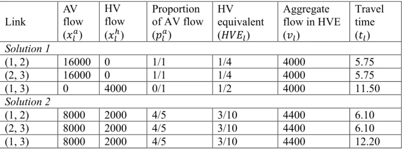
As indicated in Table 3-1, two different sets of aggregate link flows in HVE both satisfy the user equilibrium conditions. The O-D equilibrium travel times associated with the two solutions are 11.50 and 12.20, respectively. The total system travel time of the solution 2 is 6.1% higher than that of the solution 1.

Table 3-1: Flow distributions and link travel times for the toy network in the first scenario Link AV flow (𝑥_@>) HV flow (𝑥_@=₎ Proportion of AV flow (𝑝_@>) HV equivalent (𝐻𝑉𝐸_@) Aggregate flow in HVE (𝑣_@) Travel time (𝑡_@) Solution 1 (1, 2) 16000 0 1/1 1/4 4000 5.75 (2, 3) 16000 0 1/1 1/4 4000 5.75 (1, 3) 0 4000 0/1 1/2 4000 11.50 Solution 2 (1, 2) 8000 2000 4/5 3/10 4400 6.10 (2, 3) 8000 2000 4/5 3/10 4400 6.10 (1, 3) 8000 2000 4/5 3/10 4400 12.20

Scenario 2. Consider another scenario when 𝜂̅_@=> = 𝜂̅_@>> = 0.45 seconds, ∀𝑙 ∈ {(1, 2), (2, 3), (1, 3)}, 𝜂̅_@== _{= 𝜂̅}

@

>= _{= 1.8 seconds, ∀𝑙 ∈ {(1, 2), (2, 3)}, and 𝜂̅}

„´== = 𝜂̅„´>= = 1.5 seconds. The link capacities with pure HVs are 𝑐̂_„Z= _{= 𝑐̂}

Z´= = 4000 veh/h, 𝑐̂„´= = 4800 veh/h and the 𝐻𝑉𝐸@ values defined in equation (3-8) are HVE„Z = HVEZ´= 1/4, HVE_„´= 3/10. In this scenario, 𝜂̅_@==_{+ 𝜂̅}

@>>− 𝜂̅@=>− 𝜂̅@>= = 0, ∀𝑙 ∈ 𝐿 but ab_Ldd a

b_Lcc is not a link-independent constant. This scenario is also possible because: (1) controlled by computers, AVs may adopt consistent time headways on different types of links; (2) the three links are not homogeneous and HVs may adopt different time headways on them. The link capacities of links (1, 2) and (2, 3) are consistent with the base-condition value for a multilane highway segment with a 50-mi/h free flow speed in the highway capacity manual (TRB, 2016). The link capacity of link (1, 3) is consistent with the base-condition value for a freeway segment with a 75-mi/h free flow speed in the highway capacity manual (TRB, 2016)

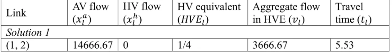
As shown in Table 3-2, two different sets of aggregate link flows in HVE both satisfy the user equilibrium conditions. The O-D equilibrium travel times associated with the two solutions are 11.06 and 11.50, respectively. The total system travel time of the solution 2 is 4.0% higher than that of the solution 1.

Table 3-2: Flow distributions and link travel times for the toy network in the second scenario Link AV flow _(𝑥 @>) HV flow (𝑥_@=₎ HV equivalent _{(𝐻𝑉𝐸} @) Aggregate flow in HVE (𝑣_@) Travel time (𝑡_@) Solution 1 (1, 2) 14666.67 0 1/4 3666.67 5.53

(2, 3) 14666.67 0 1/4 3666.67 5.53 (1, 3) 1333.33 4000 3/10 4400 11.06 Solution 2 (1, 2) 0 4000 1/4 4000 5.75 (2, 3) 0 4000 1/4 4000 5.75 (1, 3) 16000 0 3/10 4800 11.50

The above two scenarios demonstrate that the uniqueness of aggregate link flow in HVE for the user equilibrium problem cannot be guaranteed if either of the two conditions in Proposition 3-4 (i.e., 𝜂̅_@==_{+ 𝜂̅}

@ >>_{− 𝜂̅}

@=>− 𝜂̅@>= = 0, ∀𝑙 ∈ 𝐿 and ∃ 𝑎 constant 𝜆 such thatabLdd

ab_Lcc = 𝜆, ∀𝑙 ∈ 𝐿) is not satisfied.

3.1.6 Solution algorithm

Based on the travel time function defined by equations (3-7) and (3-10), we derive partial derivatives ÀÁL`}L c<sub>,}</sub> Ldf À}<sub>L</sub>c and ÀÁL`}Lc,}Ldf À}_Ld as follows: 𝜕𝑡@B𝑥@=, 𝑥@>C 𝜕𝑥_@= = 𝑡̂@𝛼@𝛽@ B𝑐̂_@=_CKL(𝑣@) KL{„𝜂̅@ ==_`B𝑥 @=C Z + 2𝑥_@=_𝑥 @>f + B𝜂̅@=>+ 𝜂̅@>=− 𝜂̅@>>C(𝑥@>)Z 𝜂̅_@==_B𝑥 @=+ 𝑥@>C Z 𝜕𝑡_@B𝑥_@=_{, 𝑥} @>C 𝜕𝑥_@> = 𝑡̂_@𝛼_@𝛽_@ B𝑐̂_@=_CKL(𝑣@) KL{„𝜂̅@ >>_B(𝑥 @>)Z+ 2𝑥@=𝑥@>C + B𝜂̅@=>+ 𝜂̅@>=− 𝜂̅@==CB𝑥@=C Z 𝜂̅_@==_B𝑥 @=+ 𝑥@>C Z 3.1.6.1 Diagonalization algorithm

Chen et al. (2017a) believe it is reasonable to assume that 𝜂̅_@=> ≥ 𝜂̅_@>> since an AV following an HV is likely to at least maintain the same headway as when it follows an HV, and that 𝜂̅_@>= _{≥ 𝜂̅}

@

== _{since a HV following an AV is likely to at least maintain the} same headway as when it follows a HV. Under this assumption, we have B𝜂̅_@=>_{+ 𝜂̅}

@ >=₋