FLOOR OPTIONS ON STRUCTURED PRODUCTS
AND LIFE INSURANCE CONTRACTS
Rami Yosef
Abstract
We consider an exotic call option defined on structured products and on two types of life insurance contracts: pure endowment insurance and risk insurance contracts. Upon exercise, these option contracts promise the higher of either the future value of the invested fund in risk-free in-terest rate, which is defined in the option contract or the future value of the fund invested in a bas-ket of risky assets. The randomness of interest rate is modulated by two stochastic processes: Orn-stein-Uhlenbeck (OU) process and the Vasicek process. In each case considered, an explicit ex-pression of the value of the options as well as numerical examples are provided.
Key words: American call option; European call option; Floor option; Ornstein-Uhlenbeck process; Pure endowment insurance; Risk insurance; Vasicek process.
1. Introduction
Banks in Israel have recently started oěering new investment avenues called Structured Products (SP). These products are designed for investors interested in investing their money in an avenue with probability of high yield to maturity, without risking their invested fund. These SP have a variety of investment paths. The most common paths are those that promise investors the higher of either the future value of the fund investedinrisk-free interest rate or the future value of the fund invested in a basket of risky assets. Such a basket of risky assets could include investment of 50% of the fund in the S&P 500, 25% in the DJ Eurostoxx 50 and the remaining 25% in KOSPI 200. On the maturity date ofthe investment in SP, the bank undertakes to pay the higher future value of either the invested fund with a deterministic interest rate as defined in the SP contract and the future value of the fund invested in these risky assets.
Motivated by the SP, we suggest an exotic option defined on SP and life insurance con-tracts. We use two types of life insurance contracts: pure endowment insurance and risk insurance. In the first case, where the exotic option is defined on the SP andonpure endowment insurance, option holders buy this option contract and deposit an amount of money, referred to as the invested fund. The invested fund is invested for a defined date to maturity. The option writer opens a cur-rent account for the invested fundand begins management of the account by investing the fund in the free market in a basketofrisky derivatives. If the option holders survive through the exercise date of the option, they could exercise the option contract and receive the higher of either the fu-ture value of the invested fund in risk-free interest rate, which is defined in the option contract or the future value of the invested fund which is invested in the basket of risky assets. The amount of money paid by the option writer upon exercise of the option contract is paid after deduction of a commission, which is a percentage of the diěerence between the future valueofthe invested fund in the risk-free interest rate and the future value of the invested fundin the risky assets. Note that op-tion holders will only exercise the opop-tion contract on the maturity date if the value of the underly-ing asset (the invested fund in the risky assets) is, at that time, worth more than the future value of the invested fund discounted by therisk-free interest rate defined in the option contract. Also note that in the option contract suggested here, if option holders do not survive through the maturity date of the option, the value of option contract is zero and the beneficiaries of the option holders do not get back the invested fund. Once the price of the option contract suggested here has beenfound, itis simple to find the value of the option contract in cases where even if option holders do not sur-vive through the exercise date, the invested fund discounted by the risk-free interest rate reverts to the beneficiaries. The following are several points worthy of mention here: a) This option contract
© Rami Yosef, 2006
could only be exercised on the maturity date of the option. This type of option contract behaves like a European type of option and is actually a floor option. b) Theoptionwriterismotivated to achieveahigh yieldtomaturity onthe investments, as the commission is defined as a percentage of the diěerence between the future value of the invested fund in risk-freeinterestrateand thefuture-value of theinvested fund which is invested in the basket of risky assets. c) If option holders decide to exercise the option on the maturity date, the option writer “buys” the underlying asset from the option holders for the present value of the invested fund, discounted by a risk-free interest rate, and “pays” the option holders the invested fund multiplied by the interest rate earnedby the basket of the risky assets after a percentage has been deducted as commission. Thusthistypeof option tract is actually a version of a European call option. Note that the strike price of this option con-tract is the future value of the invested fund, discounted by the risk-free interest rate. d) It is obvi-ous why option holders are motivated to invest inthis kind of exotic option contract instead of in the original SP oěered by the banks. Theansweris the same reason for investing in pure endow-ment insurance instead of investing in bank savings. In this type of option contract, investors ex-pect a higher yield to maturity than the investment in the original SP. e) Moreover, should option holders not survive through the exercise date, the value of the option contract is zero. This is the same as in a pure endowment insurance contract, and means that even the invested fund does not revert back to the beneficiaries. But as aforementioned, after pricing this kind of option contract, the value of this option contract can easily be found, even if option holders die during the life of the option, the future value of the invested fund with risk-free interest rate could revert back to the beneficiaries.
In the second case considered, we define an option contract on SP and risk insurance con-tracts. A risk insurance contract means that if the insureds do not survive through the maturity date of the policy contract, the beneficiaries of the insureds receive the sum assured, as defined in the insurance contract, from the insurance company. In this type of option contract defined on the SP and on risk insurance, the comments discussed with regard to the first contract hold true in this case as well. Option holders buythe option contract for fixed price, which is the price of the option. They deposit an amount of money in the option writer account, which is then invested by the op-tion writer in abasketof a risky assets. If opop-tion holders should die during the life of the opop-tion, their beneficiaries (who could be named in the option contract) could exercise the option contract and get from the option writer the future value of the invested fund discounted by the higher of the risk-free interest rate or the interest rate achieved on the investmentinthe basket of risky assets after the commission has been deducted. If option holders survive through the exercise date, they cannot exercise the option contract, and the value of this option contract is zero. Thus the option holders (their beneficiaries) lose the invested fund as well. However, as aforementioned, this op-tion contract can be underwritten, such that even if opop-tion holders survive through the exercise date, the invested fund discounted by the risk-free interest rates could revert back. Note that this exotic option is reminiscent of an American call option, both in terms of the exercise date and the strike price.
In the two cases of exotic option contracts considered here, two types of stochastic proc-esses are used to modulate the randomness in the interest rates: The Vasicek and Ornstein-Uhlenbeck ( OU) processes. In each of these stochastic processes, the prices of these options are evaluated and numerical examples are provided.
Recent studies in the actuarial literature integrate the mathematics of finance with the mathematics of insurance. Starting with unit-linked life insurance, Bernnan and Schwartz (1976) recognized the option structure of an unlinked-linked life insurance contract with a guarantee. Briys and de Varenne (1994) deal with the bonus option of the policy holder and the bankruptcy option of the (owners of the) insurance company in terms of contingent claims analysis. Other re-cent studies which deal with the bonus option are Miltersen and Persson (1998) or Grosen and JØrgensen (2000). Other contexts in which two or more stochastic processes govern the life of a put option that have been studied in the literature are the pricing of put options on defaultable bonds or swaps, and the pricing of Asian exchange rate options under stochastic interest rates. The study of options in other contexts, in which two or more stochastic processes govern the life of a
defaultable bond or swaps has a long history, but the seminal paper in this field is most likely that written by Duěy and Singleton (1997). There the riskless, instantaneous interest rate is adjusted by the firm issuing the bond or swap default hazard, to yield a model that formally resembles the de-fault-free case and that can be resolved in a similar manner. The adjustment, however, involves the sum of two hazard-like terms which implies independence, despite the fact that some type of rela-tionship likely exists between the default hazard and instantaneous interest rate. Similarly, Asian options are written on the exchange rate in a two-currency economy. In valuing these options, both the stochastic nature of the foreign and domestic zero-coupon bond prices and the exchange rate process are modeled. A recent treatment of the problem is given by Nielsen and Sandmann (2001), in which the two countries’ zero-couponbondprice processes are assumed to be independent geo-metric-Brownian motions, but the exchange rate process is modeled by a stochastic diěerential equation that is a geometric Brownian motion based on the diěerence of the short-term interest rate processes in the two countries.
Both discrete and continuous-time stochastic models for interest rate processes have been presented in the actuarial literature, primarily Gaussian autoregressive processes. Panjer and Bell-house (1980) provide a thorough review of autoregressive processes of order 1, AR(1), and of or-der 2, AR(2), with constant volatility (variance). Parker (1994), and references therein, discusses modeling the force of interest, versus modeling the accumulated force of interest, using a continu-ous-time autoregressive process of order 1: the OU process with a superimposed linear trend, and the Weiner process with linear trend. More recently, Milevsky and Promislow (2001) have mod-eled the short-rate process itself as a Cox-Ingersoll-Ross (CIR) process. The CIR process in an AR(1) process in continuous time, with random volatility that is proportional to the square root of the instantaneous interest rate just prior to time t. Other recent studies which combine call options on pension annuity insurance plans were conducted by Ballotta and Haberman (2003) and Yosef, Benzion, and Gross (2003).
The rest of this paper is structured as follows: In Section 2 we present the floor option defined on SP and on pure endowment insurance contracts. We find explicit expressions for the value of this option contract in case of the Vasicek and OU processes, which modulate the ran-domness in the interest rate process. In Section 3 we solve the case of a floor option defined on SP and on risk insurance contracts in the two cases of the stochastic processes presented above. Nu-merics and conclusions are provided in Section 4. Note that we clearly ignore expenses, profits and other administrative charges and thus assume that everything is presented on a net basis.
2. Floor Option on SP and Pure Endowment Insurance
This section focuses on evaluating the exotic call option defined on SP and pure endow-ment insurance as presented above, under the stochastic structure of the interest rates. We can write this floor option where the mortality and the interest rate are stochastic by:
>
@
¿
¾
½
¯
®
!
0 0 0 01
Pr
0
0 rt t X t rt PE SP f fe
e
E
k
e
B
t
T
C
G T , (1) wheret0 – the time from 0 to the end of the policy contract.
T – random variable describing the total lifetime of an individual.
į – constant risk-free interest intensity.
rf – the risk-free interest rate.
k – constant factor denoting the commission of the option writer.
Ĭ – constant factor.
X(t) – the random interest rate process.
0 t rf
Be
– the value of the invested fund at time 0.PE SP
C
denotes price of this exotic-floor call option defined on the SP and on pure en-dowment insurance at time 0.Note that as aforementioned, this type of option contract is actually a flooroption. At time zero, option holders pay the price of the option which is:
C
SPPE0
and also deposit an amount of money equal to0 t rf
Be
in the option writer account. If option holders survive through the exer-cise date, they can exerexer-cise the option, and the profit from exercising the option contract is>
0 00
@
1
t Xt rfte
e
BE
k
G T . Note that this option contract could only be exercised whenoption holders survive through the exercise date of the option. If they do not survive, the value of the option is zero. In this case option holders spend money to purchase the option and lose the in-vested fund as well, meaning that even the inin-vested fund does not revert back to their beneficiaries. In order to evaluate the price of an option contract in case of death of the option holder during the life of the option contract and the receipt of the invested fund by the beneficiaries, the following equation must be solved:
>
0 0 0@
01
Pr
0
0 t Xt rt rt PE SP f fBe
e
e
E
k
B
t
T
C
¿
¾
½
¯
®
!
G T , which will beeasy for evaluation after solving (1).
We assume that the stochastic structure of the interest rate follows two kinds of stochastic processes: Vasicek model and OU process. These two processes have interesting behaviors. The OU process has an advantage that its sample functions tend to revert to the initial position, a prop-erty which seems appropriate for many interest rate scenarios. The finite dimensional distributions are normal, and the process has a Markovian property (see Beekaman & Fuelling (1990,1991)). The Vasicek model has a tendency to fluctuate around fixed interest rate į> 0, with an eventually stabilizing volatility. The connection between these two processes and more about OU and the Vasicek processes will be given in the following.
Denote by X(t) the Vasicek process which is defined as a diěusion process satisfying the stochastic diěerential equation:
X
t
dt
dB
t
t
X
d
~
D
J
~
V
, (2)where (Į,Ȗ,ı) > 0 and
B
t
tt0 is standard Brownian motion with drift 0 and variance 1 per unit time (see Baxter and Rennie, 1996, p. 153). In terms of stochastic integral, the solution of (2) is given by³
X
e
t te
t sdB
s
t
X
00
~
~
J
J
DV
D . (3) According to (3),X
~
has a drift towards Ȗ of (state-dependent) sizeD
J
X
~
t
,whichis thus proportional to the distance from Ȗ. Note that for a special case, where Ȗ =0,weget the OU process. Also note that we can represent the Vasicek process by
t
X
e
t
X
~
J
(
1
Ht)
, (4)where X(t) is OU process. By Karlin and Taylor (1981, p. 332)
X
t
~
N
xe
Dt,
h
t
, whereh
t
V
2/
2
>
1
e
2Dt@
, soX
~
t
~
N
xe
DtJ
1
e
Dt,
h
t
.In this case, from (4), we can write the LT of the Vasicek process, Tt X~
*
,by:e
e
R
E
X t xe e ht t X t t
*
T
T T J T T T D D,
2 1 ~ ~ 2 . (5)Lemma 1. Let
X
~
t
follow the Vasicek process as described in (2), then we can write the size>
@
t0 X~t0rft0
e
e
E
G T by:>
@
¸¸
¸
¸
¹
·
¨¨
¨
¨
©
§
)
*
0 0 0 ~ 0 0 01
t
h
t
h
e
xe
t
r
e
t t f t X tT
J
T
G
D D T G¸¸
¸
¸
¹
·
¨¨
¨
¨
©
§
)
0 0 0 0 01
t
h
e
xe
t
r
e
t t f t rf D DJ
T
G
,where ĭ(·) is the cumulative distribution function of the normal distribution,
*
X~Tt is the Laplace Transform (LT ) of the Vasicek process which is given in (5) att
0,and where>
0@
2 2 01
2
/
e
tt
h
V
D .Proof. Denote by
d
*
X~yt the cumulative distribution function of the Vasicek process at 0t
in the point y,then for ș> 0>
@
r t Xyt t X t r y t t r t X tF
d
e
e
e
e
E
f f f 0 0 0 0 0 0 0 0 ~ ~ 1 ~³
°¿ ° ¾ ½ °¯ ° ® T G G T T G now since
X
~
t
~
N
xe
DtJ
1
e
Dt,
h
t
we can solve this integral and get:
>
@
¸¸
¸
¸
¹
·
¨¨
¨
¨
©
§
)
¸¸
¸
¸
¹
·
¨¨
¨
¨
©
§
)
*
¸¸
¸
¸
¹
·
¨¨
¨
¨
©
§
)
f³
0 0 0 0 0 ~ 0 0 0 ~ 0 0 0 0 0 0 0 0 0 0 01
1
1
t
h
e
xe
t
r
e
t
h
t
h
e
xe
t
r
e
t
h
e
xe
t
r
e
dF
e
e
t t f t r t t f t X t t t f t r y t X t r y t f f f D D D D T G D D T G T GJ
T
G
T
J
T
G
J
T
G
where 2 0 2 01
2
te
t
h
V
D .So the price of this floor option defined on SP and pure endowment insurance under the Vasicek process at time zero,
0
Vasicek PE SP
C
>
@
1
, 1 1 Pr 0 0 0 0 0 0 ~ 0 0 0 0 0 0 0 0 ° ° ° ° ¿ ° ° ° ° ¾ ½ ° ° ° ° ¯ ° ° ° ° ® » » » » » » » » » ¼ º « « « « « « « « « ¬ ª ¸¸ ¸ ¸ ¹ · ¨¨ ¨ ¨ © § ) ¸¸ ¸ ¸ ¹ · ¨¨ ¨ ¨ © § ) * ! t h e xe t r e t h t h e xe t r e k e B t T C t t f t r t t f t X t t r Vasicek PE SP f f D D D D T G J T G T J T G (6)
where
*
X~Tt is the LT of the Vasicek process which is given in (5) at the pointt
0 ,ș>0and where
>
@
0 2 2 01
2
/
e
tt
h
V
D
. Now by letting Ȗ =0, we get the price of the floor option defined on SP and pure endowment insurance under the OU process.
3. Floor Option on SP and Risk Insurance
In this section we examine pricing the value of an exotic call option defined on SP and on risk insurance under the stochastic structure of the interest rates. As previously mentioned, in this kind of option contract, option holders acquire the option for an amount of money and must de-posit an invested fund in the option writer account. The option writer starts investing this fund in a basket of risk assets such as in the stock exchange orother risky derivatives in order to achieve the best yield to maturity on the investments. In case of death of the option holders during the life of the option contract, the beneficiaries have the option of exercising the option and receiving from the option writer the higher of either the invested fund discounted by the risk-free interest rate or the discount value of the invested fund with the real interest rate achieved by the option writer through the maturity date, after a commission has been deducted. This commission is defined as a percentage of the diěerence between the risk-free interest rate and the real interest rate achieved by the option writer on the investments, multiplied by the invested fund. Furthermore, if the option holders survive through the exercise date, the worth of this option is zero. Thus the option writer is motivated to maximize this diěerence and achieve the best possible yield on the investments. Note that the death of option holders could, of course, be any time until the exercise date, meaning that the option could be exercised by the beneficiaries at any time through the exercise date. This type of option is actually a floor option that acts like an American call option in terms of the exercise date and the strike price. It is floor option since in case of death of option holders during the life of the option, the beneficiaries will, at the very least, have the invested fund discounted by the risk-free interest rate. It is also considered a call option, because if the option contract is exercised, the beneficiaries “buy” the invested fund from the option writer by “paying” the price of the future value of theinvestedfundinrisk-free interest rates, and inreturnreceive from the option writer the future value of the invested fund with the real interest rate achieved on their investments. Now the value of this floor option at time zero can be written by:
>
@
¿
¾
½
¯
®
0 0 0 0 ~
1
)
0
(
r T t T t XT t r T t RI SP f fe
e
E
e
E
k
B
C
G T , (7) wheret
0 , T, į, rf , ș, B, k,X
t
~
are as defined in the above section, and where
)
0
(
RI SP
C
is the value of this floor option at time 0 under these parameters and variables. Note that at time zero option holders pay the price of the optionC
RIPE(
0
)
and deposit an amount of money equal to 0 t rfBe
0in the option writer account. If the option holders do not survive through the exercise date, their beneficiaries could exercise the option with a gain of:
>
0 ~ 00
@
1
T t X T t rf T te
e
E
k
B
G T . Also note that should option holders survive throughthe exercise date of the option, the value of the option is zero. In this case, option holders spend money to purchase the option and lose their invested fund. To evaluate the price of an option con-tract, where even if the option holder survives through theexercisedatetheywillget back
theirin-vestedfund, thefollowing equation must be solved:
0>
0 ~ 0 0@
01
)
0
(
r T t T t XT t r T t rt RI SP f f fBe
e
e
E
e
E
k
B
C
G T ,which will be easy for evaluation after calculating (7).Now the calculation of the option contract presented in (7) under the Vasicek process which is denoted by
C
SPVasicekRI0
, is given in the following Lemma.Lemma 2. Let
X
~
t
follow the Vasicek process as described in (2). Then for ș> 0,we can write (7) by:>
@
t T t t f t t t r t T t t f t t X t t r T Vasicek RI SP
dF
t
h
e
xe
t
r
e
k
B
dF
t
h
t
h
e
xe
t
r
e
k
B
k
B
C
f f¸
¸
¸
¹
·
¨
¨
¨
©
§
)
¸
¸
¸
¹
·
¨
¨
¨
©
§
)
*
*
³
³
0 0 0 0 0 0 0 ~ 0 0 0 0 0 01
1
1
1
1
0
D D D D T GJ
T
G
T
J
T
G
(8)where
dF
Tt is the cumulative distribution function of the T , rfT
*
is the LT of T , ĭ(·) is the cumulative distribution function of the normal distribution, andT
t X~
*
is the LT of the Va-sicek process which is given in (2).
Proof. Let
W
min
>
T
,
t
0@
.Then for ș> 0,¸¸
¸
¹
·
¨¨
¨
©
§
»
»
¼
º
«
«
¬
ª
¿ ¾ ½ ¯ ® W
T W G W W W T GW W W f f f r X r X X t T r Vasicek RI SPe
e
E
E
k
B
e
E
k
B
C
~ ~ ~1
1
1
0
0 .Now the size of the conditional expectation with respect to X(IJ ), could be written by:
X r Xy t r y t r X r X Xe
e
e
e
d
F
E
f f f f W T W G W T G T W G W W W T GW WW
~ ~ 1 ~ ~ ~ 0 01
³
°¿ ° ¾ ½ °¯ ° ® °¿ ° ¾ ½ °¯ ° ® »
»
¼
º
«
«
¬
ª
>
@
¸
¸
¸
¹
·
¨
¨
¨
©
§
)
¸
¸
¸
¹
·
¨
¨
¨
©
§
)
*
W
J
T
W
G
W
T
W
J
T
W
G
DW DW W DW DW T W GWh
e
xe
r
e
h
h
e
xe
r
e
f r f X1
1
~Now since IJ = T for T< t0, and since the value of this option is 0 for T> t0, taking
expecta-tion with respect to IJ = T , weget therequired result of (7), which is givenin lemma 2.
As aforementioned, if we want to find the value of this floor option under OU process,
0
OU RI SP
C
, all that is needed is to place Ȗ =0.4. Numerics and Conclusions
We will consider two cases of the random variable of the total lifetime for an individual (T). The first case is an exponential lifetime, where Pr(T> t0)= eíIJӒt
0
for positive constants IJ, t0. The second case is Gomperz low: µage=wc
age
for positive constants w and c. In this case we can write the survival lifetime as:
¸ ¹ · ¨ © § ¸ ¹ · ¨ © §
!
0 ln 1 0Pr
t age c c c we
t
T
, where the parameter “age” refers to thepresent age of the insured. In each case we will find the prices of these floor options
Vasicek PE SP
C
, OU PE SPC
, Vasicek peC
, Vasicek RI SPC
and OU RI SPC
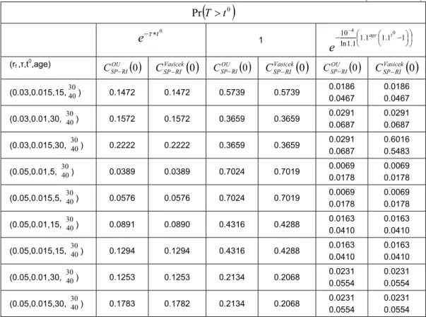
under several assumptions of the parameters. We will compare these results to thepricesof these floor options, where the probability of the insured to survive through the exercise date is 1, i.e. Pr(T> t0)= 1.
Suppose the constant parameters of the processes are: į = 0.05, ı = 0.01, Į = 0.02, ș = 0.1, Ȗ = 0.07, x0= 0.05, the bank commission is k = 10%, and B =$1.The results for some scenario
of the risk-free interest rate rf,and for some positive t
0
,IJ and the parameter age will be given in the following tables (t0is giveninyears). Also suppose that the constant parameters of the Gomperz low are: w =10í4,c =1.1.Table 1 presents the values of the floor options defined on SP and on pure endowment insurance contracts, and Table 2 presents the results of the floor options defined on SP and on risk insurance contracts.
Table 1 outlines the prices of the floor options defined on SP and on pure endowment in-surance. As mentioned in Section 2, at time zero option holders pay the price of the option CSP íPE(0) and deposit an amount of money equal to:
0 t rf
Be
to the option writer account. If the op-tion holders survive through the exercise date, they can exercise the opop-tionC
SPPE0
and theirprofit from exercising the option contract is
>
@
0 0 0
1
t Xt rfte
e
BE
k
G T .Note that all of numerics are for B =$1. If, for example, we examine the case where the constants are rf= 0.03,IJ = 0.01, t
0
=5 (5 years), age =30, the prices of the option contract in case of the OU and Vasicek processes is $0.8187 in the exponential case. This means that option holders will only have a gain from exercising this option contract if the annual interest rate achieved by the option writer on the investments exceeds 12.707%.
Table 1 Prices of the floor options on SP and on pure endowment insurance
0 PrT !t 0 te
W 1 ¸ ¹ · ¨ © § ¸ ¹ · ¨ © § 1 1 . 1 1 . 1 1 . 1 ln 10 4 age t0e
(rf,IJ,t0,age) OU 0 PE SP C Vasicek 0 PE SP C CSPOUPE 0 Vasicek 0 PE SP C CSPOUPE 0 Vasicek 0 PE SP C (0.03,0.01,5,3040) 0.8187 0.8187 0.8607 0.8607 0.8511 0.8361 0.8511 0.8361 (0.03,0.015,5,3040) 0.7985 0.7985 0.8607 0.8607 0.8511 0.8361 0.8511 0.8361 (0.03,0.01,15, 3040) 0.5488 0.5488 0.6376 0.6376 0.6016 0.5483 0.6016 0.5483 (0.03,0.015,15, 3040) 0.5092 0.5092 0.6376 0.6376 0.6016 0.5483 0.6016 0.5483 (0.03,0.01,30, 3040) 0.3012 0.3012 0.4066 0.4066 0.3008 0.1862 0.3008 0.1862 (0.03,0.015,30, 3040) 0.2592 0.2592 0.4066 0.4066 0.3008 0.1862 0.3008 0.1862 (0.05,0.01,5, 3040) 0.7412 0.7411 0.7793 0.7791 0.7706 0.7570 0.7704 0.7568 (0.05,0.015,5, 3040) 0.7229 0.7228 0.7793 0.7791 0.7706 0.7570 0.7704 0.7568 (0.05,0.01,15, 3040) 0.4070 0.4068 0.4729 0.4726 0.4461 0.4066 0.4459 0.4064 (0.05,0.015,15, 3040) 0.3776 0.3774 0.4729 0.4726 0.4461 0.4066 0.4459 0.4064 (0.05,0.01,30, 3040) 0.1655 0.1654 0.2234 0.2232 0.1653 0.1023 0.1652 0.1022 (0.05,0.015,30, 3040) 0.1425 0.1423 0.2234 0.2232 0.1653 0.1023 0.1652 0.1022 Table 2 Prices of the floor options on SP and on risk insurance 0 PrT!t 0 te
W 1 ¸ ¹ · ¨ © § ¸ ¹ · ¨ © § 1 1 . 1 1 . 1 1 . 1 ln 10 4 age t0e
(rf,IJ,t0,age) OU 0 RI SP C Vasicek 0 RI SP C OU 0 RI SP C Vasicek 0 RI SP C OU 0 RI SP C Vasicek 0 RI SP C (0.03,0.01,5,3040) 0.0408 0.0408 0.7746 0.7746 0.0073 0.0187 0.0073 0.0187 (0.03,0.015,5,3040) 0.0604 0.0604 0.7746 0.7746 0.0073 0.0187 0.0073 0.0187 (0.03,0.01,15, 3040) 0.1015 0.1015 0.5739 0.5739 0.0186 0.0467 0.0186 0.0467Table 2 (contionuous)
0 PrT!t 0 te
W 1 ¸ ¹ · ¨ © § ¸ ¹ · ¨ © § 1 1 . 1 1 . 1 1 . 1 ln 10 4 age t0e
(rf,IJ,t0,age) OU 0 RI SP C Vasicek 0 RI SP C OU 0 RI SP C Vasicek 0 RI SP C OU 0 RI SP C Vasicek 0 RI SP C (0.03,0.015,15,3040) 0.1472 0.1472 0.5739 0.5739 0.0186 0.0467 0.0186 0.0467 (0.03,0.01,30, 3040) 0.1572 0.1572 0.3659 0.3659 0.0291 0.0687 0.0291 0.0687 (0.03,0.015,30, 3040) 0.2222 0.2222 0.3659 0.3659 0.0291 0.0687 0.6016 0.5483 (0.05,0.01,5, 3040) 0.0389 0.0389 0.7024 0.7019 0.0069 0.0178 0.0069 0.0178 (0.05,0.015,5, 3040) 0.0576 0.0576 0.7024 0.7019 0.0069 0.0178 0.0069 0.0178 (0.05,0.01,15, 3040) 0.0891 0.0890 0.4316 0.4288 0.0163 0.0410 0.0163 0.0410 (0.05,0.015,15, 3040) 0.1294 0.1294 0.4316 0.4288 0.0163 0.0410 0.0163 0.0410 (0.05,0.01,30, 3040) 0.1253 0.1253 0.2134 0.2068 0.0231 0.0554 0.0231 0.0554 (0.05,0.015,30, 3040) 0.1783 0.1782 0.2134 0.2068 0.0231 0.0554 0.0231 0.0554Table 2 indicates the prices of the floor option defined on SP and on risk insurance con-tracts. If we take, for example, these constant parameters rf=0.05,IJ =0.015, t
0
=30, we can see that the prices of this option contract with OU process in case of a certain lifetime is $0.2134 andin-caseof the Vasicek process is $0.2068. The prices of this option in the exponential case is $01783 in the OU process and $0.1782 with the Vasicek process. Additionally note that some diěerences exist between the option prices under Gomperz low of mortality and the exponential case, pre-dominantly due to the lack of memory with regard to the age of the insured parties attributed to the exponential lifetime.
5. Conclusions
In this paper we introduce a floor option defined on SP and on life insurance contracts. These option contracts could lead insurance companies, if we think of them as option writers, to be more involved in the capital market, an objective important to all parties involved, particularly in a country as small as Israel. Furthermore, in Israel, all insurance policies with a component of sav-ings on the reserves of the policies, such as pure endowment insurance, endowment insurance and annuity insurance contracts, have to investapercentage of their portfolio in risky assets. They benefit from a commission which is a percentage of the gain of their investments, but they also enjoy a fixed commission even if they have bad investments. Thus the kind of contracts suggested here is also very important to the insured parties interested in buying an insurance contract with a savings element such as pure endowment insurance and would like to protect their invested fund from bad investments of the insurance companies. These contracts will also accelerate the compe-tition between the insurance companies to maximize the profit from their investments.
References
1. Ballotta, L., Haberman, S., (2003). Valuation of Guaranteed Annuity Conversion Options. Insurance; Mathematics and Economics, 33, pp. 87-108.
2. Baxter, M., Rennie, A., (1996). Financial Calculus, Cambridge University Press.
3. Beekaman, J.A., Fuelling, C.P., (1990). Interest and Mortality Randomness in Some Annui-ties. Insurance: Mathematics and Economics, 9, pp. 185-196.
4. Beekman, J.A., Fuelling, C.P., (1991). Extra Randomness in Certain Annuity Models. Insur-ance; Mathematics and Economics, 10, pp. 275-287.
5. Bernnan, M.J., Schwartz, E.S., (1976). The Pricing of Equity-Linked Life Insurance Policies with an Asset Value Guarantee. Journal of Financial Economics, 3, pp. 195-213.
6. Briys, E., De Varenne, F., (1994). Life Insurance in a Contingent Claim Framework: Pricing and Regulatory Implications. The Geneva Papers of Risk an Insurance Theory, 19, pp. 53-72. 7. Grosen, A., JØrgensen, P.L., (2000). Fair Valuation of the Life Insurance Liabilities: The Im-pact of the Interest Rate Guarantees, Surrender Options, and Bonus Policies. Insurance: Mathematics and Economics, 26, pp. 37-57.
8. DuĜe, D., Singleton, K., (1997). An Econometric Model of the Term Structure of Interest Rate Swap Yields. The Journal of Finance, 52, 4, pp. 1287-1321.
9. Karlin,S., Taylor, H.M., (1981). A Second Course in Stochastic Processes, 2nd. Ed. Aca-demic Press, Inc. New-York.
10. Milevsky, M.A., Promislow, D.A., (2001). Mortality Derivatives and Option to Annuities. Insurance: Mathematics and Economics, 29, pp. 299-318.
11. Miltersen, K., Persson, S.A., (1998). Guaranteed Investment Contracts: Distributed Excess Return. Technical Report. Department of Finance, University of Odense.
12. Nielsen, A.J., Sandmann, K., (2002). Pricing of Asian Exchange Rate Options Under Stochas-tic Interest Rates as a Sum of Options. Finance and StochasStochas-tics, 6, pp. 355-370.
13. Panjer, H.H., and Bellhouse, D.R., (1980). Stochastic Modelling of Interest Rates with Appli-cations to Life Contingencies. Journal of Risk and Insurance, 47, pp. 91-110.
14. Parker, G. (1994). Two Stochastic Approaches for Discounting Actuarial Functions. Astin Buletin, 24, 2, pp. 167-181.
15. Yosef, R., U. Benzion, and S.T. Gross, 2004, Pricing of a European Call Option on Pension Annuity Insurance, Journal of Insurance Issue, 27, 1, pp. 66-82.