Evaluating Tropical Upper-tropospheric Water in Climate Models Using Satellite Data

(1)

THESIS FOR THE DEGREE OF DOCTOR OF PHILOSOPHY

Evaluating Tropical Upper-tropospheric Water in

Climate Models Using Satellite Data

MARSTON S. JOHNSTON

Department of Earth and Space Sciences

CHALMERS UNIVERSITY OF TECHNOLOGY

(2)

MARSTON S. JOHNSTON ISBN 978-91-7385-958-5

©MARSTON S. JOHNSTON, 2014.

Doktorsavhandlingar vid Chalmers tekniska h¨ogskola Ny serie nr 3640

ISSN: 0346-718X

Department of Earth and Space Sciences

Global Environmental Measurements and Modelling Chalmers University of Technology

SE - 412 96 Gothenburg, Sweden Phone + 46 (0)31 772 1000

Cover: Observed and simulated cloud fraction anomalies for land-based deep convective systems in the tropics, _±3° latitude, _±10°longitude, and _±48 hours from the center point of peak surface precipitation.

Printed by Chalmers Reproservice Chalmers University of Technology Gothenburg, Sweden 2014

(3)

To the two stars in my heaven:

Adam Oliver Sebastian Johnston

and

Emma C. Andersson

(4)

MARSTON S. JOHNSTON

Department of Earth and Space Sciences Chalmers University of Technology Abstract

Measuring and simulating moist processes in the tropical upper troposphere are difficult tasks. Humidity in this region of the atmosphere is mainly supplied by deep convection and, problems with simulated convection are known to be a major contributor to uncertainties in climate model projections. Observations within this region of the atmosphere are hampered by the low absolute humidity as well as by the presence of clouds.

This thesis examines the seasonal changes in and the effects tropical deep convection have on upper-tropospheric water, in addition to its effect on outgoing longwave radiation (OLR). Multiple satellite observations are assessed and used to evaluate the climate models EC-Earth, CAM5, and ECHAM6. The data are analysed using two main methods: longterm averages and compositing. Compositing represents an improvement over climatologies because it brings the comparison closer to the processes associated with deep convection. The compositing method is adapted fromZelinka and Hartmann [2009], improved, and applied for the first time to climate models.

Upper-tropospheric humidity (UTH) undergoes large seasonal and regional changes in the tropics. Over land areas, convection is more intense, producing greater amounts of water at higher heights, and having a greater effect on the OLR. Corresponding model simulations capture the large-scale and seasonal changes, however there are significant inconsistencies when compared with the observations, especially over land regions. Simulated mean UTH in areas where DC systems develop are consistently higher than observed over both land and ocean. However, the direct response of UTH to DC systems is found to be similar to the observations. Modeled cloud fractions near the tropopause are tend to be overestimated, whereas ice water content is often too low. The observed OLR can, regionally, differ from the simulated results by as much as 20 W m−1. Moreover, above and around deep convection systems, the local decrease of OLR is throughout underestimated. Further, the models all demonstrate a lack of spatial variability indicated by a diurnal repetition of convection at the same location over land. These results obtained by the composite method reveal details that could not have been obtained using a traditional climatology based comparison.

(5)

Keywords: Climate, IWC, Humidity, Clouds, ECHAM6, CAM5, EC-Earth

(6)

(7)

Appended papers

The thesis is based on the following articles:

• Johnston, M. S., Eriksson, P., Eliasson, S., Jones, C. G., Forbes, R. M., and Murtagh, D. P.: The representation of tropical upper tropospheric water in EC Earth V2, Clim. Dyn., 39, 2713-2731, doi:10.1007/s00382-012-1511-0, 2012.

• Johnston, M. S., Eliasson, S., Eriksson, P., Forbes, R. M., Wyser, K. and Zelinka, M. D.: Diagnosing the average spatio-temporal impact of convective systems Part 1: A methodology for evaluating climate models, Atmos. Chem. Phys., 13, 13653-13684, doi:10.5194/acpd-13-13653-2013, 2013.

• Johnston, M. S., Eliasson, S., Eriksson, P., Forbes, R. M., Gettelman, A., R¨ais¨anen, P. and Zelinka, M. D.: Diagnosing the average spatio-temporal impact of convective systems – Part 2: A model inter-comparison using satellite data, Atmos. Chem. Phys. (submitted).

(8)

(9)

Related papers

Paper in which I have participated but not appended to this thesis:

• P. Eriksson, B. Rydberg, M. Johnston, D. P. Murtagh, H. Struthers, S. Ferrachat, and U. Lohmann. Diurnal variations of humidity and ice water content in the tropical upper troposphere. Atmos. Chem. Phys. 10:11519-11533, 2010. DOI 10.5194/acp-10-11519-2010.

(10)

(11)

Acknowledgments

This work is in collaboration with, and partially funded by, the Rossby Centre, Department of Research and Development, Swedish Meteorological and Hydrological Institute (SMHI).

I would like to express my gratitude to my colleagues at Global Environmental Measurement and Modelling group and the Rossby Centre at SMHI for their support. Special thanks to Colin Jones, Klaus Wyser, Martin Evaldsson for their extra support to make this thesis a reality. Special thanks is also reserved for my advisor, Patrick Eriksson, it has not always been an easy road, but much of this work would not be possible without your ideas and help.

(14)

(15)

Chapter

1 Introduction and Overview

This chapter attempts to give a brief overview and some history of the current concern for the planet’s climate system. This is an enormously broad and complex topic and cannot be fully addressed here. The following sections highlight some main points and milestones in climate research as they pertain to this thesis. Ultimately, I try to highlight the connection between observations and simulation of the climate systems and the need to improve climate models, all in an effort to better understand the legacy of the Anthropocene1_.

1.1 Earth’s climate system

When considering the climate of the Earth, many factors come into play - both external and internal to the planet. External factors governing the climate include the energy provided by the sun, which is one of the basic factors of planetary climate. Our proximity to the sun largely determines the amount of incoming radiation, which falls unequally on the planet as a function of latitude. Changes in the incoming solar radiation depend on changes in the solar cycle as well as changes in the planets orbital properties. These changes occur at times scales that ranges from a decade to many thousands of years.

The different systems on the planet, mainly the ocean, land, ice, vegetation, and the atmosphere react to the incoming radiation and interact with each other to redistribute the differential solar heating. Therefore, the climate of the Earth is described as a system of interconnected sub-systems with feedbacks that can amplify or dampen the effect of changes in the incoming

1_{An informal geologic chronological term that marks the evidence and extent of human}

impact on the Earth’s ecosystems.

(16)

radiation. This is an example of internal forces controlling the global climate. For millennia, the redistribution of the incoming solar energy has served to balance planetary heat loss with the heat gain and has kept the global temperature at around 288 K.

The climate of a particular region is generally defined as the statistics of the weather over a time frame of about 30 years. It can be described as, for example, the expected average temperature, rainfall, humidity, or cloudiness depending on the time of year. Around the planet, the climate close to the surface ranges from cold near the poles, temperate in the middle latitudes, and warm in the tropics. Therefore, the climate of a region depends largely on its latitude. Other factors also control the climate of a region, these include its height above sea level, its proximity to water and the properties of that water body, and orography, to name a few.

The evolution of the climate system is governed by physical principles that, if they are well known and we know the initial state of the climate, it would be possible to produce a climate projection that has little or no statistical uncertainty. But the factors that govern the climate’s evolution are not well known and we cannot measure all the climate’s systems in full detail. Nevertheless, the climate does lend itself to statistical descriptions. Nonlinear processes in the climate system act to amplify disturbances in such a manner that predictability is lost after a certain time. However, there are dissipative processes in the climate system, such as surface friction, that acts to keep it within certain predictable boundaries.

Changes in the climate that last for decades and beyond are considered significant and can originate from within the climate system and/or from external forces. The planet’s climate has always changed. This has been verified by geological records of past climate states2_{. Changes in past climate}

have shown that any change in the energy balance between the incoming and outgoing radiation will initiate a change. Examination of past climate change has verified climate’s sensitivity to changes in the global atmospheric CO₂ concentrations. Over the last century changes in the climate have occurred more rapidly than before. The burning of fossil fuels increases the atmospheric concentration of CO₂ together with deforestation and other changes in land use have been identified as some examples of human activities changing internal factors that govern the planet’s climate and leading to an unequivocal global warming. In order to understand the ongoing changes to the climate system, observations and simulations of past and future climates are studied.

Future climate projections designed to assess the impact of anthropogenic

(17)

1.2. Carbon dioxide and the greenhouse effect 5 effect on the climate system are not without a number of uncertainties. There are three primarily causes to such uncertainties. The first is the presence of incomplete knowledge and limited understanding of, for example, climate physics, which limit the accuracy of climate models. The second cause of uncertainties arises from the natural variability of the climate system, both simulated and observed, and has an inherent unpredictability that can sometimes mask the effects of climate change. The final uncertainty stems from unknown future of socio-economic trends. This thesis is falls within the realm of the first uncertainty source.

1.2 Carbon dioxide and the greenhouse effect

Observations of the Earth and its climate system have been ongoing for millennia, but collecting and analyzing observational data did not become systematic until the early 20th century. Over the next 100 years, Earth observations have evolved from ground-based sensors, human observers, and simple cameras to high-altitude airborne crafts and later on to its next natural step, space-borne satellites. To date, the planet’s hydrosphere, biosphere, atmosphere, and lithosphere all have dedicated observational platforms that include measurements of atmospheric gaseous species such as CO₂, O₃, H₂O, land use, ice thickness, and sea surface temperature.

In the late 19th _{century it was not yet known what governed the onset and} termination of the planet’s various ice ages. The concept ofgreen house effect3 was put forth as an explanation as to why the Earth is so warm at the surface (_∼15◦C) given its distance from the sun4_{. Building on this theory, Svante}

Arrhenius5, in 1896, theorized that changes in the concentration CO₂, a well-mixed atmospheric gas, could affect the global mean temperature. His theory implied a proportional relationship between this trace gas and the global mean temperature via a formulation that is still used today: ∆F =αln(C/C0), where ∆F is the radiative forcing, in W m−2, C is the global atmospheric CO₂ concentration in parts per million volume (ppmv), C0 is a baseline reference for global atmospheric CO₂ concentration (typically a pre-industrial concentration value of 280 ppmv), and αis a constant between five and seven [Myhre et al., 1998].

Arrhenius formulation assumes radiative equilibrium between the incoming solar radiation and the outgoing longwave radiation [Manabe, 1997]. He

3_{http://en.wikipedia.org/wiki/Greenhouse_effect}

4_{This region of space within which the Earth orbits is commonly known as the}_Goldilocks

or habitable zone.

(18)

predicted that a doubling of CO₂ concentrations could change the global mean temperature by_∼5◦C. While this value would be adjusted for feedback processes, Arrhenius did not take into account other effects from, for example, clouds or convection. Nevertheless, with this simplified example model of the climate system, Arrhenius considered that anthropogenic emission of CO₂ would change the planet over a period of several millennium and prevent a new ice age, an overall positive view, then, of the anthropogenic CO₂ effect. Up until the mid 20th century, Arrhenius theory was not widely accepted and neither was it without controversy. Some argued that the atmosphere was already saturated with CO₂, while others argued that ocean would absorb all anthropogenic emission. The former argument was based on observation of CO₂ taken within the planetary boundary layer and very close to its source. The latter argument was based on estimates of global emissions, as there were no global measurement of atmospheric CO₂ until the mid 1950s. The need for global atmospheric observations is therefore critical in order to understand the concept of greenhouse gases and the current and projected effect on the climate system with any change in their concentrations.

1.3 Climate sensitivity

In order to understand the response of the global climate system to forcings both internal and external, we need to determine the system’s sensitivity to such forcings. Climate sensitivity, expressed in ◦C, is a fundamental aspect of the system and is normally determined with regards to the change in the planet’s radiation balance brought about by a doubling of atmospheric CO₂. In atmosphere-ocean climate models, climate sensitivity is function of the synergy between many aspects of the model, for example, its physics. However, simpler energy-balance models use a climate sensitivity that is defined differently. In this case, climate sensitivity,λexpressed in◦C/(W/m2), translates a particular radiative forcing, ∆F, into a change in the global surface temperature, ∆T, after equilibrium in the climate systems has been reached (∆T =λ_×∆F).

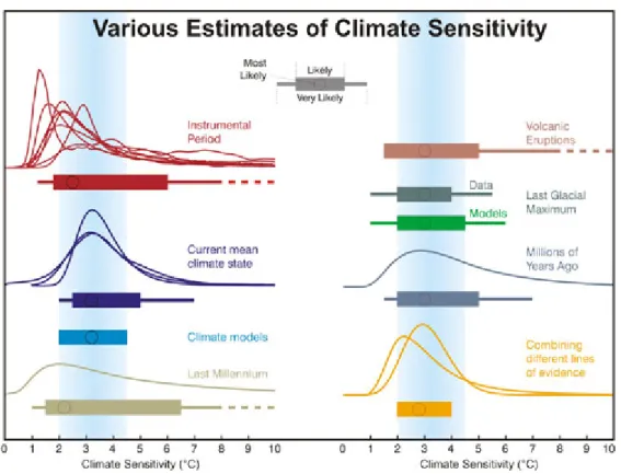
Quantifying the planet’s climate sensitivity to a doubling of CO₂ has proven to be a difficult task. Climate sensitivity calculated using observations from recent past, going back millennia, and using model-simulated data have been able to establish a lower limit with good confidence. Uncertainties in the climate forcing and the physics of the system’s response make establishing a upper bound difficult and create extreme cases and outliers [Knutti and Hegerl, 2008, Fig. 3]. Climate sensitivity obtained from an ensemble of simulated climate projections is called effective climate sensitivity as models do not

(19)

1.3. Climate sensitivity 7

Figure 1.1: Climate sensitivity from several sources. The most likely values are depicted by circles, likely values are given bars (>66 % probability), and very likely are shown as lines (>90 % probability). Dashed lines indicate no robust constraint on an upper bound. Distributions are truncated in the range 0 – 10 K. The IPCC likely range and most likely value are indicated by the vertical grey

bar and black line, respectively. Source: original from Knutti and Hegerl [2008] but this adapted example can be found athttp: // www. skepticalscience. com/ climate-sensitivity-advanced. htm.

run long enough to reach equilibrium state. Figure 1.1illustrates the various climate sensitivity values obtained from models and observations as well as an estimate derived from a combination of the different lines of evidence. While the range for the climate sensitivity discussed is simply based on forcing caused by changes in CO₂ concentrations, it nevertheless gives us an idea of what to expect for changes in the global temperature caused by other types of forcing.

(20)

1.4 Observations

Observations are critical in the understanding of the climate system. Although ground-based observations of atmospheric CO₂ have existed since the late 19th _{century, they were not very precise nor were they reliable. It was not} until Charles Keeling6 established a monitoring station at the Mauna Loa Observatory in 1956, that the world’s first benchmark for global atmospheric CO₂concentration was created. Since then, proxy observations have confirmed that the planet’s climate is ever changing and ice core measurements of atmospheric CO₂ concentrations over the last 200 years has risen at rates not seen during the last _∼500 000 years7_{. At the rate of approximately 2}

ppm per year (2013)8, this atmospheric trace gas has risen from about 280 ppm about 100 years ago [Keeling,1997] to roughly 395 ppm as of Dec 20139_.

Fig.1.2 shows the timeseries of CO₂ concentrations for the last half century. The rate of increase is highly correlated to the increase in human energy consumption and population increase. The Mauna Loa Observatory is a single ground station, and, in order to monitor the planet, the next logical step was space-borne satellites. Remote sensing observations of the planet’s climate system came of age with the advent of satellites, but it was not until the mid 1990s that satellites dedicated to monitoring the Earth’s climate were launched. Measurements of atmospheric infrared emission, microwave emission, reflected ultra-violet, and visible light are all part of the current global observing system. While observations tell us what is going on in the climate system, they are only snapshots in time. What is desired is a forecast of the future climate, and general circulation (climate) models, largely because they can simulate feedback processes, are the best tool for quantifying changes to come.

1.5 General circulation models

The idea of a numerical model was first postulated by Bjerknes et al. [1904] based on the assumptions that subsequent atmospheric states develop from a proceeding one in a manner that is governed by physical laws. If the interaction between the systems involved is sufficiently well known and their initial states can be ascertained with enough accuracy, then a future atmospheric state can be simulated. But it was not until the 1950’s, when computers were

6_{http://en.wikipedia.org/wiki/Charles_Keeling}

7_{https://www.ipcc.ch/publications_and_data/ar4/wg1/en/tssts-2-1-1.html} 8_{http://www.esrl.noaa.gov/gmd/ccgg/trends/}

(21)

1.5. General circulation models 9

Figure 1.2: Timeseries “Keeling curve” of global atmospheric CO₂ from 1956 to April 2013. Superimposed on the figure, bottom right, is the annual cycle. Source:

http: // en. wikipedia. org/ wiki/ Keeling_ Curve.

used to solve numerically the equations governing the atmosphere, that the first forecast was made. Climate models evolved out of numerical weather predictions models and are able to run for hundreds of years. In order to represent the climate, each sub-component of the climate system need to be simulated. Some of the first climate models could not fully represent the radiative balance between the sun and the Earth because convection was not represented [Manabe and Strickler, 1964; Manabe and Wetherald,1967]. Over the years, and in step with advancements in computer processing and observations, more sub-components have been added to climate model. Today, there can be an atmospheric, ocean, land-surface, sea ice, vegetation, and chemistry component present in a climate model. One advantage of complex models is that they are able to simulate the feedbacks found in the climate system, which is necessary to determine the climate sensitivity. However, as the complexity of climate models increases it has the undesired effect of making them harder to evaluate.

(22)

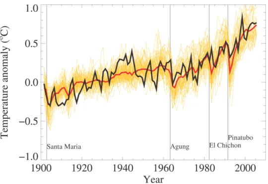
Figure 1.3: Mean global near-surface temperature for the past century. Obser-vations (black) are plotted together with 58 simulations (yellow) produced by 14 different climate models. The mean of all these runs is also shown (thick red line). Vertical grey lines indicate the timing of major volcanic eruptions. Source: IPCC

Fourth Assessment Report.

1.6 Model evaluation

GCMs are able to capture observed features of past and recent climate changes. Together with available observations as constraints, the climate system sen-sitivity can be better assessed, which enables us to better understand the response of the climate system to external and/or internal forcing. However, we are still unable to significantly improve on Svante Arrhenius prediction of

≈5 K increase in the global mean temperature for a doubling in the global atmospheric CO₂ concentration. It is estimated that if CO₂ concentrations were to reach 580 ppmv, the planet will likely see a temperature rise _∼3◦C (see Fig. 1.1), but this improvement of the _∼5◦C advanced by Arrhenius is

not without a degree of statistical uncertainty, extremes, and outliers. Some tests that are performed on climate models are:

1. Simulations for the recent past 50 – 150 years, where the mean state, climate changes, and variability at various timescales, for example, are examined.

(23)

1.7. International Panel on Climate Change 11 2. Paleoclimate modelling, where the last glacial maximum and millenium

are exmined.

3. Idealized test such as a doubling of global atmospheric CO₂ concentra-tions are exmined

Figure1.3 illustrates the ability of models to simulate past climate. However, a climate model’s performance cannot be easily ascertained when projecting, e.g., 100 years into the future. Instead, confidence is gained by judging the accuracy of recent and past climate scenarios - but this is insufficient. In order to increase model fidelity, reduce the statistical uncertainty in future climate projections, and improve the estimates of climate sensitivity, models need to undergo comprehensive evaluations on identified areas of weakness. By subjecting models to rigorous tests on multiple levels, errors can be identified and corrected [Randall et al.,2007]. Models need to subjected to more tests that evaluate the inner workings.

Today, GCMs are evaluated in many more ways; in particular, components can be compared (so called component level), or via system level where the model output is compared. Another more useful method involves ensembles of output from a number of models in order to study the lower and upper bounds of the possible climate projections in response to a specific forcing. System level evaluations can be carried out using a model to retrieval comparison or by simulated satellite radiances with the aid of a satellite simulator such as Cloud Feedback Model Intercomparison Project (CFMIP) Observation Simulator Package (COSP) [Bodas-Salcedo et al., 2011]. Both model to retrieval and simulated radiance methods have advantages and disadvantages when trying to bring both the model and the satellite definitions as close to each other as possible. However, when studying cloud feedback processes, a satellite simulator is often employed. Special focus is often given to a region, or regions, of any of the climate’s sub-system previously identified as problematic as well as any particular model output. One such region is the upper troposphere where observations are limited, and an example of a variable is the representation of clouds, which is considered one of the largest source of model uncertainty [Randall et al.,2003].

1.7 International Panel on Climate Change

Global warming is unequivocal, and the view of most scientist today is that the effects of a rapid increase atmospheric CO₂ concentrations, to levels of 400 ppm and beyond, are not positive. For example, the melting of the polar ice caps will lead to a change in the planet’s albedo, the oceans are becoming

(24)

more acidic due the absorption of high amounts of CO₂, are effects that are threatening much of the life on the planet. In order to understand the effects of increased concentrations of greenhouse gases, one needs to understand the processes involved and how they affect each other. This tantamount to understanding how the global carbon cycle functions, and it follows that only then can we fully understand how anthropogenic changes in CO₂ will affect the future climate. Climate change on such a scale is not a simple task and so the United Nation created the Intergovernmental Panel on Climate Change (IPCC) for the assessment of climate change. Every few years the IPCC publishes a report that updates the current science and conclusions regarding global warming. A part of the IPCC report consists of the results of a Coupled Model Intercomparison Project (CMIP) within which many models from many research centers around the world compare standardized outputs. Coupled to the CMIP data is the Atmospheric Model Intercomparison Project (AMIP), which is a dataset where only the atmospheric component of a GCM is run, using boundary conditions. Data from the AMIP archive is meant only for scientific evaluation of models and provides freely data from many modelling centers around the world.

1.8 Tropical upper troposphere

The importance of CO₂ has been discussed so far, but another important greenhouse gas is water vapor. Water vapor is the most dominant natural greenhouse gas and is responsible for the largest positive feedback in the climate systems [Soden and Held,2006]. Any change in this atmospheric con-stituent is important for future climate projections. In the free troposphere10, CO₂ is a well mixed gas, but water vapor varies greatly and decreases with height as the temperature decreases, according to the Clausius-Clapeyron equation. In the upper troposphere, the cold temperatures keep the water vapor at low concentration levels, but as the planet warms, the water vapor content of the troposphere will increase. The absorptivity of water vapor is proportional to the logarithm of its concentration [Soden et al., 2005] therefore, in regions of the troposphere with low concentrations, fractional increases can give rise to large absorption of radiation, which can cause a significant feedback into the climate system [Solomon et al., 2007, Chap. 8 Box 8.1]. This underpins the necessity for understanding the observed moist processes in the upper troposphere and their projected changes.

(25)

1.9. Objective and structure 13

1.9 Objective and structure

The objective of the thesis is to summarize and give an overview of the work underpinning three appended papers that are concerned with the following: 1. Assessing measurements of upper-tropospheric water and its

represen-tation in the climate model EC-Earth

2. Diagnosing the spatio-temporal effect of deep convection on upper-tropospheric moist processes using a composite technique and demon-strating the technique’s viability to do the same in the climate model EC-Earth version 2

3. Expanding the objective in item 2 to include an inter-comparison be-tween EC-Earth version 3, CAM5, and ECHAM6

Chapter 1 gives some background information on the work presented in this thesis. Chapter 2provides a brief overview of tropical convection. Chapter 3

provides general review of satellite remote sensing and observation systems employed. Chapter 4 gives overview of the current state of climate models and finally, Chapter 5 presents a summary and outlook.

(26)

(27)

Chapter

2 Tropical Convection

This chapter gives a brief description of the tropics and one of its most impor-tant weather phenomenon: moist convection. The discussion on convection is later limited to deep convection, which is the focus of this thesis. Much of this chapter is based on the books Smith[1997] and Holton [1994].

2.1 The Tropics

The astronomical definition of the tropics is the area between _±23.5°latitude, but in this thesis, it is defined using the more meteorologically meaningful definition of _±30° latitude. The tropics are important in many ways, and one major aspect is the amount of incoming solar radiation. Figure 2.1shows the annual mean net longwave and net shortwave radiation per latitude. From the figure it is clear that the tropics get a surplus of energy.

This excess energy is stored in the atmosphere and ocean before being transported towards the poles. The transport of energy polewards within the oceans and atmosphere teleconnects the tropics to the remainder of the planet and gives this region special importance. Dynamically speaking, the main difference between the tropics and the rest of the planet is the magnitude of the Coriolis parameter: f = 2Ω sinθ, where Ω is the rotation speed of the planet and θ is the latitude. In the tropics the Coriolis parameter is small.

In the tropics many weather phenomena have a diurnal cycle of about 24 hours and occur on local- to meso-scale (_∼5 km and_∼100 km). A particular important region of tropical disturbances is a zonally (east to west) oriented band called the InterTropical Convergence Zone (ITCZ). The ITCZ forms where the northeast and southeast trade winds converge. Over land regions, the seasonal movement of this band follows the sun, but over the oceans, this

(28)

Figure 2.1: Annual mean net outgoing longwave radiation (red) and net incoming shortwave radiation (blue) per latitude. Source: http://www.physicalgeography. net/fundamentals/7j.html

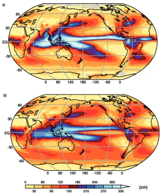
movement is smaller. In Figure 2.2the ITCZ becomes visible by looking at a longterm mean of precipitation in the region. The top plot shows the observed mean (1980 – 1999), and the bottom plot shows a simulated representation. The figure clearly shows concentrations of precipitation over the western Pacific and Indian ocean south of India.

The energy source for tropical disturbances is in the form of convection, which is the primary weather generating process in the region and mainly concentrated along the ITCZ. Observations and experiments have shown that energy balance in the tropics is achieved with the aid of convection, hence the tropics is in radiative-convective balance, more so than the mid-latitudes or the poles. Therefore, more than any other place on the planet, convection is important in the tropics [Manabe and Strickler,1964;Manabe and Wetherald, 1967].

(29)

2.2. Cumulus convection 17

Figure 2.2: Observed and simulated mean annual precipitation (1980 to 1999). Observed (a) and simulated (b), based on the multi-model mean. Source: IPCC AR4

2.2 Cumulus convection

In the tropics cumulus, or moist, convection is the conduit by which water, heat and momentum are transported from the planetary boundary layer vertically to the tropopause – and even the lower stratosphere. However, only a small portion of the total convective activity reaches the tropopause. Convection plays a fundamental role in the atmospheric energy cycle, the water cycle, and the global climate. The evolution of convection basically follows three

(30)

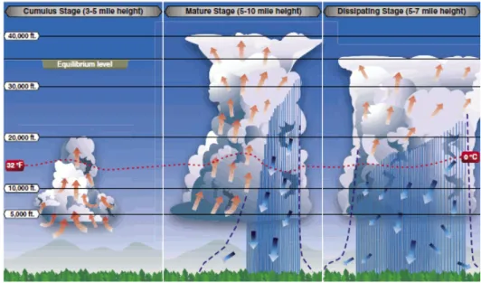
Figure 2.3: The three typical stages in the life cycle of convection. Source: http: // www. aero-mechansic. com/ wp-content/ uploads/ 2011/ 10/ 11-23. gif.

stages: cumulus, mature, and dissipating. As cumulus clouds grow, they pass through several known phases of development with special nomenclatures to indicate these new cloud forms. From the initial small cumulus cloud one sees on a fair weather day, these innocuous clouds then grow into tall towering cumulus and then cumulus congestus, achieving greater vertical penetration with each phase. In the final phase, cumulus clouds are called cumulonimbus with a signature fanning out of it cirrus shield to form an anvil-like top. Figure 2.3 illustrates the three major stages of cumulus development. In the initial stage (cumulus stage) convection occupies a very small spatial domain,

∼1 km2_{, and can grow and organize into aggregations with a coverage of}

∼1000 km2. The mature stage follows the cumulus stage, where convection reaches its maximum vertical height and precipitation begins. Finally, there is the dissipation stage where mainly precipitation occurs and the vertical velocities are almost totally negative. The maximum precipitation rates occur in the dissipation stage. The duration of convection varies depending on the underlying surface, usually land or water, where land-based convection tends to be shorter in duration.

A cumulus cloud has a complex structure consisting of several short-lived, individual plumes of rising air called thermals. These thermals are accelerated vertically and are non-hydrostatic, non-steady, and turbulent. As these plumes rise within the cloud, they carry, among other things, moisture and latent heat, which entrain into the cloud, modifying it through mixing. Positive

(31)

2.2. Cumulus convection 19 buoyancy, or instability, of the air in these thermals is dependent upon its density, which is affected by the environmental lapse rate. The lapse rate is defined as the rate of change of the temperature of atmosphere with height: dT /dz, whereT is the atmospheric temperature andz is the geometric height. Also, the instability depends on the rate of mixing of air within the plume with the surrounding environment and on the water vapour and condensates in the cloud.

The stability of the atmosphere is important for cumulus convection. The atmosphere can be said to be in a metaphysical state, where potential energy is stored until released to give rise to violent convection – typically found in the midlatitudes. However, in the tropics, such violent convection is rare at best, which means that such a build of potential energy is smaller in magnitude. Therefore, forecasting tropical convection involves forecasting the evolution of such an energy source as well as a triggering agent. The energy source for convection is the availability of potential energy to a parcel until it reaches a level of neutral buoyancy. This is defined as the Convective Available Potential Energy (CAPE):

CAP E _≡ Z LN B z Bdz = Z LN B z g Tv (Tvp−Tv)dz = Z p LN B Rd(Tvp−Tv)dlnp,

where B is the buoyancy force per unit mass, Tv is the virtual temperature,

Tvp is the virtual temperature of a adiabatically displaced air parcel, p is

pressure, Rd is the gas constant for dry air. LN B stands for the level of

neutral buoyancy.

CAPE describes the kinetic energy an unstable parcel of air can attain as it rises through the atmosphere, if mixing is ignored and the parcel adjusts instantaneously to the local environmental pressure. However, CAPE is simply an indicator of the strength of convection. If the amount is low, the convection will be weak. What determines if convection is initiated or not depends largely on the vertical shear1 _{of the horizontal wind near the surface.}

The buoyancy of an air parcel depends on its density, which depends on the amount of water present in it. The virtual temperature is used to account for the presence of water and water condensates in an air parcel. If water vapor is increased/decreased at a constant temperature, the positive buoyancy and the virtual temperature increase/decrease. There is no simple way to measure the buoyancy of a rising air parcel. In processes involving a rising/subsiding air parcel, there are many atmospheric variables that are conserved. However, there is none that is a good measure of the buoyancy of

(32)

a saturated, cloudy air parcel with respect to an unsaturated environment. Therefore, assessing the stability of moist convection must be done by other means, for example, the thermodynamic diagram, or computers, which is an estimate at best.

In the tropics CAPE is usually weak, so the release of latent heat fills the gap as the primary energy source for convection. This dependence on evapo-ration connects convection to the surface heating from the diabatic process of solar insolation. Convection releases latent heat into the atmosphere and creates a local response in the atmospheric circulation and excites equatorial waves. This creates a strong connection between tropical convection and the mesoscale and the large-scale circulation found in this region.

2.3 Equatorial waves

Some examples of equatorial waves that interact with convection via the exchange of latent heat are Equatorial Kelvin (EK), Equatorial Rossby (ER), and Mixed Rossby-Gravity (MRG) waves2_{. EK waves are trapped at the}

equator and move eastward depending on whether or not convection is as-sociated with them. These waves are fast moving if there is no convection, between_∼30 m s−1 and 60 m s−1, but significantly slower if there is accompa-nying convection, between_∼12 m s−1 and 25 m s−1. Convection is often found embedded in EK over, for example, the wester Pacific and Indian oceans. The typical description of ER waves are alternating low and high pressure areas that are symmetric about the equator. Unlike EK waves, these waves move westwards between_∼10 m s−1 and 20 m s−1 without accompanying convection and between _∼5 m s−1 and 7 m s−1 otherwise. The dissipation of energy via MRG helps to sustain convection that are strong enough to reach the UT. These waves also move westward between _∼8 m s−1 and 10 m s−1.

2.4 Deep convection

The larger the cloud, the greater the effect it will have on the atmosphere. Con-vective clouds that penetrate the tropical boundary layer inversion, and whose level of neutral buoyancy lies at pressure levels .200 hPa (10 km and 17 km), are called deep convective clouds [Folkins and Martin,2005]. Deep convection can come from a single cloud or from organised cloud systems called clusters.

2_{See the MetEd Comet Program module on Equatorial Waves:} _https:

//www.meted.ucar.edu/tropical/synoptic/MJO_EqWaves/navmenu.php?tab=1& page=2.2.0&type=flash

(33)

2.5. Tropical circulations 21 These clouds, or cloud systems, often reach levels of the UT where the cloud top temperature is .235 K. Since the anvil cloud from deep convection often covers an area large enough to be resolved by many satellites, deep convection is often identified by its cloud top temperature, [see e.g., Liu et al., 2007; Mapes and Houze, 1993; Soden and Fu, 1995, and references therein]. Further, since most of the precipitation in the tropics comes from deep convection [eg. Folkins and Martin, 2005; Hong et al., 2005], there is a strong correlation between the surface rain rate and such cloud systems. The factors that determine if a cumulus cloud grows into a deep convective cloud include the presence of low-level convergence (typically found in the ITCZ), enough CAPE, and the level of humidity in the column, especially in the lower troposphere (closely associated with the sea surface temperatures).

2.5 Tropical circulations

Large-scale circulation systems in the tropics have different characteristics from those found outside the region. The are several main large-scale circula-tions within the tropics. In addition to the ITCZ, which has already been discussed, these circulations are equatorial waves disturbances, African wave disturbances, tropical monsoons, Walker circulations, and the El Ni˜no and the southern oscillation (ENSO).

Equatorial wave disturbances are transitory and move zonally within the ITCZ in the form of organised precipitation and sustained high level of cloudiness. Such waves are driven by the release of latent heat from condensating water inside deep convective clouds. This connection between deep convective clusters and equatorial waves is too complex to fully explore in this thesis. Cursively, equatorial waves contain the largest number of deep convective clusters and provide aprotected environment for an air parcel to rise without much environmental entrainment, thus enabling deep convection to transport a large amount of latent heat and mass to near-tropopause levels.

While tropical waves disturbances behave similarly for most of the region, over Africa, the presence of the Sahara desert creates a strong baroclinic3

environment in the lower troposphere. This baroclinic zone, which is present during the strong diabatic heating of the summer months, gives rise to an easterly jet stream. Observations show that disturbances over the continent tend to move westward following this jet. Hurricanes that move through the Caribbean are often formed from these disturbances. One notable feature of African waves is that they draw energy from the conversion of energy between

3_{Baroclinic air masses are ones where the air density depends on both temperature and}

(34)

the local baroclinic zone of the easterly jet and the general barotropic4 environment of the tropics.

Monsoons are periods of heavy precipitation that are driven by the land and ocean temperature contrast. A monsoon will occur where the hotter, rising air over land creates a low pressure area (heat low) of convergence that pulls in warm, moisture laden air from offshore. This onshore flow is seasonal and generates a large amount of precipitation where they occur. Monsoons are most pronounced over southeast Asia and the Indian sub-continent.

Walker circulation describes a circulation that is zonal in orientation (east-west). This circulation is driven by tropical deep convection and are caused by longitudinal variations in sea surface temperatures, which are themselves driven by changes in wind-driven ocean currents. Variations in the Walker circulation have been given the name ”Southern Oscillation”. During the Southern Oscillation changes in the wind-stress patterns over the oceans induce a circulation change that pushes cold water to warm areas and visa versa. This change in the ocean circulation and the subsequent sea surface temperatures has been given the name El Ni˜no. These two phenomena are often referred to jointly as ENSO so as to address the total circulation system.

All of the above circulations interact with deep convective clusters at vary-ing length and time scales, which allows for a modification of the environment of the local convective area. Such time and length scale modifications often involve moisture transport, momentum transfer, etc., and involve complex, two-way relationships between tropical waves and convection that are clouded in uncertainty (see Thuburn[2011, Fig. 1.1] for an illustration).

4_{Barotropic fluid is a fluid whose density is a function of only pressure. In the atmosphere}

this translate to a region where the air temperature is fairly uniform over a broad horizontal area.

(35)

Chapter

3 Satellite observations

In this thesis, several satellite observations, mainly polar-orbiting, are used in the evaluation in climate models. Satellite observations provide global coverage of the planet remotely and on a regular basis. This chapter gives a general overview of the satellite observations used in this thesis.

3.1 Satellite observations

Satellite measurements provide information of atmospheric and surface prop-erties such as vertical profiles of temperature, trace gas concentrations, and cloud cover, in addition to surface precipitation, and radiation at the top of the atmosphere. These variables are measured using active lidar and radar sensors as well as optical, passive infrared, and passive microwave sensors.

Satellite sensors cannot measure the atmospheric quantities mentioned above directly. But the emission, absorption, and scattering of electromagnetic energy by constituents in the atmosphere allow for the derivation of geophysical parameters by interpreting the signal measured by the sensor. When the information required cannot be taken directly from the measurements, then the desired physical parameter needs to be retrieved. An inversion method is used to reconstruct the atmospheric state and derive the variable sought from the measured signal. A major complication is the fact that there can be many atmospheric states that give rise to the same measured signal. It is often the case that there are insufficient data to provide a unique solution to the atmospheric state. Some key elements of this inversion process are weighting functions and averaging kernels that vary in characteristics for each sensor type and measurement technique. Unfortunately, remote sensing observations suffer from errors, aliasing, and other limitations that introduce a degree of

(36)

uncertainty in satellite inversion results.

The measurement of atmospheric and surface variables is carried out by several different satellite sensors that also employ various techniques. The measurement of atmospheric temperature employs passive sensors that detect radiation emitted by, e.g., CO₂ at 15µm. CO₂ is an ideal candidate because it is a uniformly distributed gas, and, therefore, its thermal emission is assumed to be a function of temperature for a given pressure. Another atmospheric gas that can be used to measure the vertical temperature profile is O₂.

Atmospheric water exists in all three phases, although the majority exists as a highly variable trace gas. In certain atmospheric conditions water vapor, liquid water, and ice can exist simultaneously, which complicates satellite measurements of water in its individual phases. Humidity profiles are measured using both microwave and infrared techniques. However, since the amount of water vapor that can exist in a parcel of air is bounded by the temperature via the Clausius-Clapeyron equation, in cold regions of the atmosphere water vapor concentration is low. This further complicates the measurement of humidity. Atmospheric humidity is sometimes retrieved as specific humidity, which is the absolute amount of water vapor, expressed in, for example, kg kg−1, or volume mixing ratio, expressed as part per million (ppmv). Another way to the define water vapor is by relating it to the relative humidity expressed as a ratio of the actual vapor pressure to the saturation vapor pressure, either with respect to ice or with respect to water. Relative humidity with respect to ice is used throughout this thesis.

Clouds are strong absorbers of thermal infrared radiation, and they are good at scattering radiation in the optical band. Atmospheric ice is found mostly inside clouds and contribute to the cloud’s radiative properties. Both clouds and cloud ice can be measured passively and actively.

Passive emissions of microwave energy from the surface of the planet and the atmosphere are used to retrieve surface precipitation intensity. Infrared cloud-top temperatures (cloud heights) are correlated to surface precipitation to provide an additional measurements of surface precipitation. These various sources are combined to give full coverage of rainfall across the tropics.

3.2 Atmospheric infrared sounder

The Atmospheric Infrared Sounder (AIRS) provides height resolved humidity profiles [see e.g., Gettelman et al., 2006, 2010]. The horizontal resolution is approximately 45 km and the vertical resolution decreases with height from about 1 km near the surface to roughly 3 km near the tropopause. The sensor flies in a sun-synchronous polar orbit and crosses the equator (ascending and

(37)

3.3. Microwave limb sounder 25 descending nodes) at roughly 13:30 and 01:30 local solar time.

Specific humidity is retrieved from the sensor measurements and then converted to relative humidity using a Groff-Gratch formulation for saturation vapor pressure. A significant drawback to the AIRS humidity data is its sensitivity to cloud, which strongly absorbs infrared emissions. Consequently, humidity profiles are only available in situations where the cloud fraction is

≤70 %. Further limitations have resulted in the retrieved humidity values being only scientifically useful at pressure levels &200 hPa [Gettelman et al., 2006]. These limitations on the data mean that AIRS does not provide full coverage of the upper troposphere nor is it usable when examining deep convective clouds systems.

3.3 Microwave limb sounder

The Microwave Limb Sounder offers the opportunity to measure upper-tropospheric humidity in the presence of clouds [Fetzer et al., 2008; Read et al.,2007]. The sensor measures microwave thermal emission from the upper troposphere and above at a frequency of 190 GHz. Its vertical resolution is roughly 4 – 6 km and has a horizontal resolution of 200 – 300 km and 6 – 12 km, along and cross track respectively. The sounder also sits in a sun-synchronous orbit with ascending and descending nodes similar to AIRS. Height resolved humidity profiles suitable for scientific study are obtained for pressure levels between 383 hPa and 0.002 hPa. Measured specific humidity is converted to relative humidity in a similar manner to AIRS.

3.4 AMSU-B and MHS

Similar to the MLS sensor, the Advanced Microwave Sounding Unit-B (AMSU-B) radiometer measures atmospheric microwave emissions. This is done for different altitudes using 5 channels (89.0_±0.9, 150.0_±0.9, 183.31_±1.00, 183.31_±3.00, and 183.31_±7.00 GHz). However, AMSU-B is downward-looking, whereas MLS is a limb (sideways-looking) sounder. AMSU-B are standard sensors onboard the National Oceanic and Atmospheric Admin-istration (NOAA) and the European Space Agency polar-orbiting, sun-synchronous satellites. Microwave Humidity Sounder (MHS) is the next generation of AMSU-B sounder measuring atmospheric microwave emissions between 89 GHz and 190 GHz. In this thesis, AMSU-B and MHS are treated in a similar manner.

(38)

[Buehler and John, 2005;Buehler et al., 2008]. A linear equation is used to map the sensor measurements to relative humidity, but for these retrievals, the interpretation is not straightforward. The weighting functions are dependent on the atmospheric state; thus, in drier conditions, the measurement is representative of altitudes lower down in the atmosphere. Therefore, this mapping of the sensor signal to humidity is not defined for only one specific altitude. Consequently, AMSU-B/MHS humidity is defined as a weighted mean for the upper troposphere.

3.5 Cloud profiling radar

A cloud profiling radar measures backscatter reflectivity as a function of distance to a cloud or ice particle. The CloudSat satellite employs such a radar to measure atmospheric hydrometeors at 94 GHz (3 mm) with a vertical resolution of about 240 m and a horizontal resolution of _∼2 km [Stephens et al., 2002]. The CloudSat retrieval algorithm is described in Austin et al. [2009]. The satellite is placed in a sun-synchronous polar orbit with equatorial crossing (ascending/descending) times of approximately 13:30/01:30 local. The sensor’s sensitivity to precipitation is size dependent such that, the larger the ice particles, the greater the backscattered signal. This sensitivity limits CloudSat’s usefulness in the upper troposphere where ice particle sizes are small.

While CloudSat can penetrate any cloud to reveal its 2-D structure, there is unfortunately a 40 % retrieval uncertainty, which is a result of marginal information on the ice particle size distribution. Additional uncertainty is caused by the sensor’s inability to detect the phase of the hydrometeor generating the backscattered signal. The partition between liquid water and ice, a part of the retrieval process, is a linear function of temperature. Above 273 K, the profile is assumed to contain only liquid water whereas below 253 K, solid ice is assumed.

3.6 Cloud profiling lidar

Cloud-Aerosol Lidar with Orthogonal Polarization (CALIOP) is a polarization-sensitive lidar that measures vertical profiles of aerosols and clouds [see e.g., Chepfer et al., 2010; Winker et al., 2007]. Profiles are measures using two channels to measure polarized backscatter signal at 532 nm wavelength and another at 1064 nm. The sensor is onboard the CALIPSO satellite and detects clouds with an optical depth<0.01. Because of its high sensitivity to optically

(39)

3.7. TMPA 27 thin clouds, the CALIOP sensor saturates quickly in cloud conditions. Cloud profile of the upper troposphere is obtained by combing cloud information from CloudSat and CALIOP.

3.7 TMPA

More than 60 % of the planet’s rainfall occurs in the tropics, which is also the region with the most incoming shortwave radiation. Water releases a large amount of energy when it changes phase, and the tropics attain radiative-convective balance by the release of latent heat transported aloft during convective events. This cycle of evaporation and condensation is an integral part of the hydrological cycle and mapping the cycle of rainfall in the tropics is very important. The Tropical Rainfall Measuring Mission (TRMM) employs visible, infrared, and microwave sensors to measure rainfall in the region. Surface rain gauge measurements are then used to validate the remotely sensed rain estimation techniques.

Three rain measuring instruments fly onboard the TRMM satellite: 1. Visible and Infrared Scanner provides high resolution observations on

cloud coverage, cloud type, and cloud top temperatures.

2. TRMM Microwave Imager provides integrated column precipitation, cloud liquid water, cloud ice, rain intensity, and type of precipitation. 3. Precipitation Radar measures the 3-D precipitation.

The satellite is placed in a relatively low orbit that is not sun-synchronous. The low inclination of the satellite orbit provides coverage between _±35° latitude, a choice to give greater coverage of the tropics. However, complete spatio-temporal coverage of the tropics is not attainable with just one satellite. The Tropical Rainfall Measuring Mission (TRMM) Multisatellite Precipitation Analysis (TMPA) [Huffman et al., 2007] combines precipitation data from many more sensors to obtain a tropical precipitation analysis with a high spatio-temporal resolution (0.25°_×0.25° at 3-hour intervals). Other polar-orbiting sensors that contribute to the TMPA dataset are NOAA’s AMSU-B, Special Sensor Microwave Imager (SSM/I) on Defense Meteorological Satellite Program satellites, and Advanced Microwave Scanning Radiometer-Earth Observing System (AMSR-E) on the Aqua satellite. Together, these satellites are still not able to obtain full spatio-temporal coverage of the tropics. Precipitation data derived from infrared sensors onboard geo-synchronous earth orbit satellites fill in the gaps and allow the TMPA dataset to provide full spatio-temporal coverage.

(40)

3.8 CERES

Radiation at the top of the atmosphere is measured by the Clouds and the Earth’s Radiant Energy System (CERES) [Loeb and Kato, 2002]. This in-strument is based in a previous inin-strument called Earth Radiation Budget Experiment (ERBE). CERES is a scanner housing three detectors that mea-sure shortwave radiation (0.3₋5.0µm), longwave radiation 8₋12µm, and total radiation (0.3₋100µm) channel. The sensor flies onboard two satellites, Terra and Aqua, and crosses the equator at 10:30/22:30 local solar time for Terra and 13:30/01:30 local solar time for Aqua. The sensor scans from limb to limb cross-track and scans along track using a 360° azimuth biaxial scan.

3.9 Sampling error

Convection in the tropics an integral part of this thesis. An important aspect of convection in this region is its diurnal cycle, which requires consistent spatio-temporal coverage in order to be resolved properly. However, this is often not the case for polar-orbiting satellites, especially those in sun-synchronous orbits [Kirk-Davidoff et al.,2005], e.g., CloudSat. This low-frequency diurnal sampling causes random errors and biases in retrieved atmospheric variables associated with convection. Increasing the diurnal sampling greatly reduces this problem, however, consideration must also be given to the sensor’s scanning pattern. Because the composites used in this thesis cover a broad geographical area, sensors with narrow swaths will not adequately cover the composite’s spatial domain, which further contributes to aliasing effects.

(41)

Chapter

4 Atmospheric General Circulation

Models

This section gives a very brief description of the numerical model used to approximate the atmospheric component of a climate model. The section is limited to just a few aspects of this model component as they pertain to the subject of this thesis.

4.1 Background

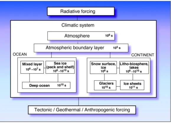
The average weather pattern of a region defines its climate and does this in terms of the longterm mean and variability of, for example, temperature, precipitation, and wind. Theclimate systemis an interactive system consisting of the atmosphere, lithosphere, hydrosphere, and biosphere. Energy from the sun drives the climate system and changes in this system are caused by internal (e.g., changes in greenhouse gas concentrations) and external (e.g., volcanic eruptions or solar variations) forces. As these forces are applied to the climate system, its responses can both be direct or indirect via feedback mechanisms. The response in these systems all occur at different temporal and spatial scales. Figure 4.1 show the typical response time to changes in the climate system.

Future climate projections require knowledge of key climate system com-ponent processes and the interactions between them. In the atmosphere, governing equations that describe the conservation of mass, momentum, and energy are expressed in a numerical environment called a model. Atmospheric general circulation models are therefore numerical systems that describe the processes necessary to simulate the climate system component.

(42)

Figure 4.1: A schematic representation of the domains of the climate system showing estimated response times. Source: McGuffie and Henderson-Sellers [2005].

There are several types of models that can be used to study the atmo-spheric climate component. Some examples are, in order of increasing com-plexity, energy balance models (EBM), radiative-convective models (RCM), statistical-dynamical models (SDM), and atmospheric general circulation models (AGCM) [Meehl, 1984]. EBMs and RCMs are often used to study the global energy exchange, the planet’s effective emissivity, and atmospheric profile. SDMs are usually a combination of a EBM and a RCM but with increased dimensions. AGCM may be run using prescribed boundary con-ditions instead of being coupled with other models such as an ocean or ice model. But any study of the real climate can only be done using a AGCM coupled to models that describe the other climate system components (see Fig. 4.1).

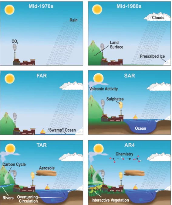
Since the mid 1950s, climate models have become increasingly complex by trying to incorporate more and more systems and processes thereby signifi-cantly increasing the number of equations, and parameterizations. Figure 4.2

illustrates the evolution of climate models since the early 1970’s. The ever increasing complexity of AGCMs is needed to simulate a climate system with multiple interactions and feedbacks. At the same time, the increased

(43)

4.1. Background 31 complexity makes interpreting model output more difficult.

Figure 4.2: Evolution of general circulation models since the 1970’s. The added parameterizations (physics) are shown pictorially by the different features of the modelled world. Source: IPCC WG I

(44)

4.2 Dynamics and physics

AGCMs must contend with the dynamics of a fluid on a rotating planet, the physics behind each process, the energy balance between the planet’s outgoing longwave and the incoming shortwave radiation, plus the redistribution of energy throughout the atmosphere. At any point in time, AGCMs represent winds, atmospheric density, pressure, temperature, and humidity. This is the dynamics of the model and is concerned with mass continuity, water conservation, momentum, and internal energy. In the governing equations, there are four independent variables: time (t), height above sea-level, or geopotential (Φ), longitude (λ), latitude (φ). There are seven dependent variables, namely horizontal velocities east-west v and north-south u, vertical velocity ω, density, ρ, mass water (ice, liquid, and vapour) q, temperature, θ, and pressure,p.

With seven dependent variables there are therefore seven basic equations climate models must solve for the atmosphere on a rotating Earth. Atmo-spheric motions caused by differential heating from the sun are solved using the momentum equation. If we let U~ represent the vector components of velocities (v, u, ω) and Ω is the rotation speed of the planet, then the three dependent variables can be solved using the expression

d ~U dt =−2Ω× ~ U | {z } Coriolis −1 ρ∇p |{z} PGF +~g+F~r, (4.1)

where the first term is the Coriolis effect, the second is the pressure gradient force (PGF), third term is the net force of gravity that includes centrifugal force, and last term is frictional drag. This is an atmospheric expression of Newton’s second law of motion (F~ =m~a) and includes an advection term (_dtd = _∂t∂ +U~ _{· ∇}).

Another equation for the fourth dependent variable ρ describes the con-servation of mass and states that the local rate of change of density is equal to minus the mass divergence is given by

∂ρ

∂t +∇ ·(ρ ~U) = 0, (4.2)

where ρ is the local atmospheric density. A third equation describes the conservation of constituents such as water mass and represents one of the most difficult aspects of modelling. The implementation of these equations vary from model to model and an example can be written for specific humidity q as

(45)

4.2. Dynamics and physics 33 ∂ρq ∂t =−∇ ·| {z(ρq ~U)} Advection + E₋ρC | {z }

Source & Sink

, (4.3)

where E is a evaporation/sublimation, and C is condensation/deposition. This flux form for water mass conservation (using Eq. 4.2), represents a balance of temporal and spatial changes with sources and sinks. In models such EC-Earth, where the treatment of precipitation is diagnostic, humidity and cloud water (e.g., ice and liquid combined), or cloud ice and cloud liquid water, would be represented by two such equations.

A fourth equation describes the thermodynamics that governs the conser-vation of energy with respect to a moving air parcel defined as

Q=Cp dθ dt − 1 ρ dp dt, (4.4)

where Cp is the specific heat capacity, and Q is the heating rate per unit

mass. The equation of state p=ρRT is the final equation and describes the relationship between temperature, pressure, and density for an ideal gas.

These governing equations are solved for each time step as well as spatially but are limited by computational cost and processing time in order to make modelling the atmosphere practical. The next step to solving the governing equations involves some necessary approximations that are standard in climate models. Some approximations are the hydrostatic relation:

ρg =₋dp

dz, (4.5)

where, g is acceleration due to gravity and ρ is the density, that states that at large spatial scales, typically >10 km, vertical acceleration is negligible; the vertical component of the Coriolis effect can be ignored; and the quasi-Boussinesq approximation that states: variations in atmospheric density in time are very small compared to other components of Eq.4.2, which in effect filters out sound waves.

The governing equations so far do not address some important aspects of the atmosphere such as clouds and radiation. Therefore, more equations that describe missing elements are added. At this point, the model system is not closed since the energy dissipating frictional force, F~r, and heating rates

from the sun and the Earth’s surface, mixing, as well as transport of heat that arises from phase change in water are still unspecified. To account for heating from the sun, the cooling of the planet, phase change heating and cooling from primarily convection a radiative-convection transfer model is

(46)

added. The addition of clouds, convection and radiation are often referred to as the model physics.

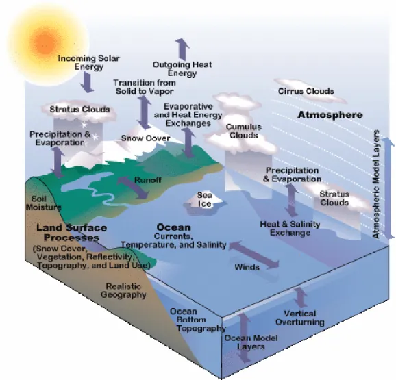
As mentioned earlier, AGCMs solve the governing equations on spatial and temporal scales that are partially determined by computational costs and numerical limitations. These scales are, today, on the order of tens to hundreds of kilometres with time steps from several minutes to about an hour. Without the above limitatons, the equations being solved can provide information down to_∼cm scale and on times steps on the order of seconds. This disparity between what the model scale resolves from the equations, plus the fact that many important variables, such as clouds, occur at multiple scales, including scales well below 50 km (resolution of next generation AGCMs), require the addition of more equations. Any additional equations to the original seven is one form of parameterization (Sect.4.3). These types of parameterizations require closure that is achieved when boundary conditions that describe the interactions of other components of the climate system are added. Figure 4.3

illustrates the different components of several major climate systems and the processes that must be represented.

4.3 Parameterization

In order to adequately represent the atmosphere in a numerical model, the basic governing equations need to be supplemented with equations that describe other processes that are not covered but are equally important. These additional equations are calledparameterizations.

Parameterizations can be described as simplified models of unresolved processes that can be measured or not. An example of parameterization is convection that account for the vertical transport of momentum, heat, and total water. A second type of parameterization is radiation, which involves processes that affect molecular internal energy, a kind of diabatic process, i.e., absorption/emission of photons and phase changes. The third kind of param-eterization in AGCMs are additions to the governing equations. Examples of these are land surface scheme, carbon cycle, clouds effect, chemistry, and aerosols. Parameterizations in AGCMs reflect, from their design, use, and implementation, our understanding of the processes they describe. Many of these processes are not well understood and therefore parameterizations be-come a source of uncertainty in AGCMs. Thuburn [2011, Fig. 1.1] illustrates the gap that parameterizations must bridge in the models. The darker-shaded areas, that represent spatio-temporal scales of various models, are noncon-tiguous, but the lighter-shaded area, that represents nature, is contiguous. Parameterizations bridge the gaps between these darker areas. AGCMs today

(47)

4.4. Clouds 35

Figure 4.3: Typical numerical model domain for a coupled system. Source: NCAR CCSM

have a typical resolution of_∼100 km and a time step of about _∼1 h. This puts current AGCM resolutions at the same level as cloud clusters.

4.4 Clouds

The role of clouds in the atmosphere is complex and broad. Clouds affect the 3-D dynamics, temperature, humidity, radiation, and the water budget in the atmosphere. The effects of clouds on the global climate depend on their amount, location, height, lifespan, and optical properties. The radiative impact of clouds is not only dependent on the above cloud properties, but

(48)

Cloud-Radiation Interaction Cloud fraction

and overlap

Cloud top and base height Amount of condensate In-cloud condensate distribution Phase of condensate _Cloud particle size Cloud particle shape Cloud environment Cloud microphysics External influence Cloud macrophysics

Figure 4.4: Cloud-radiation interaction, the processes involved, and the scale at which they occur. Red: microscale, yellow: macroscale, grey: quantum scale.

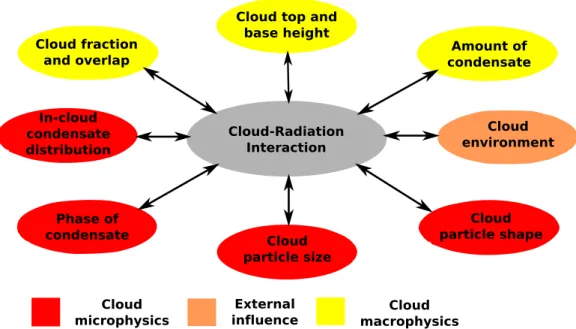
also the time of year and day. The optical properties and radiative impact are also dependent on the presence of aerosols.

Simulating clouds and cloud effects are very difficult tasks that many AGCMs solve in a similar manner but with small yet significant differences. It is common to link the cloud formation to the relative humidity as it rises above a particular threshold, and the interaction with aerosols is often simplified, if represented at all. Explicit cloud representation has only been implemented in AGCMs since the early 1980s based on work by Sundqvist [1978]. The effect of clouds in models is usually encompassed in three processes: cloud fraction, cloud microphysics, and cloud radiative properties [Kiehl et al.,1998]. Figure 4.4 shows an example of the processes involved in cloud-radiation interaction and the scales on which they occur. However, micro-properties of clouds exist at scales that are smaller than the resolutions of contemporary AGCMs. Therefore, many AGCMs employ parameterizations (see Sect. 4.3) to describe these sub-grid properties. Parameterizations of clouds describe statistical properties of a cloud field, but neglect individual cloud elements. The goal, however, is to simulate the clouds as realistically as possible. Because many of the processes involving clouds are still poorly understood, cloud parameterization is the largest source of uncertainty in AGCMs [Bony et al., 2006].

Evaluating Tropical Upper-tropospheric Water in Climate Models Using Satellite Data